Atomic motion in tilted optical lattices

Abstract

This paper presents a formalism describing the dynamics of a quantum particle in a one-dimensional, time-dependent, tilted lattice. The formalism uses the Wannier-Stark states, which are localized in each site of the lattice, and provides a simple framework allowing fully-analytical developments. Analytic solutions describing the particle motion are explicit derived, and the resulting dynamics is studied.

1 Introduction

A recent revival of interest on the old problem of electron motion in perfect, non-dissipative, periodic lattices Bloch_States_ZFP28 ; Zener_BlochOsc_PRSA34 is due to the advent of laser cooling techniques, that have opened the possibility of realizing the interaction of atoms with perfect, non-dissipative, optical lattices. Optical lattices are a consequence of the displacement of atomic levels resulting from the interaction with light CCTHouches90 ; MeystreAtOpt . A far-detuned standing wave formed by two counter-propagating laser beams (of wave-vector $k_{L}$) is perceived by an atom as a one-dimensional potential $V$, whose strength varies sinusoidally in the space: $V\propto\cos(2k_{L}x)$ (where $x$ is the spatial variable). Standing waves are the model potential considered in the present work. The main source of dissipation in such lattices is spontaneous emission, which can be reduced in a controlled way by increasing the laser-atom detuning. By scanning the frequency of one of the beams forming the standing wave with respect to the other, one can generate an accelerated potential. In the (non-inertial) frame in which the standing wave is at rest, an inertial constant force appears, producing a “tilted” lattice. This technique can also be used to modulate (temporally) the position or the slope of the potential. Tilted optical lattices generated in this way have been used for recent experimental observations of Bloch oscillations both with atoms Salomon_BlochOsc_PRL96 or Bose-Einstein condensate Arimondo_BECBlochOsc_PRL01 . Wannier-Stark ladders Raizen_WSOptPot_PRL96 and collective tunneling effects Kasevich_BECTiltedLattice_Science98 have also been studied with such a system.

A very convenient theoretical framework for studying atom dynamics in a tilted lattice is that formed by the so-called Wannier-Stark (WS) states Wannier_WS_PR60 , which are the eigenstates of a tilted lattice Korsch_LifetimeWS_PRL99 ; AP_WannierStark_PRA02 . In particular, we have studied in a previous work the quantum dynamics in a time-modulated, tilted lattice using such basis Nienhuis_CoherentDyn_PRA01 ; AP_WannierStark_PRA02 . In the present paper, we present exact solutions of the equations of motion obtained in Ref. AP_WannierStark_PRA02 that describe the atomic center of mass motion. Sec. 2 briefly reviews the main properties of WS states leading to a simple description of Bloch oscillations; Sec. 3 studies the coherent dynamics in a modulated lattice, leading to a general equation of motion; we derive in Sec. 4 an exact solution for the equation of motion which is studied and characterized in Sec. 5.

2 The Wannier-Stark basis

Let us first introduce natural units in which lengths are measured in units of the lattice step $d$ ($=\lambda_{L}/2$, $\lambda_{L}$ $=2\pi/k_{L}$ being the laser wavelength), energy is measured in units of the “recoil energy” $E_{R}=\hbar^{2}k_{L}^{2}/(2M)$ where $M$ is the atom mass, and time is measured in units of $\hbar/E_{R}$. The Hamiltonian corresponding to a tilted lattice is then:

$$H_{0}=\frac{P{{}^{2}}}{2m}+V_{0}\cos(2\pi x)+Fx$$ (1)

where $m=\pi^{2}/2$ is a reduced mass, $F$ is a constant force measured in units of $E_{R}/d$, the momentum operator in real space is $p=-i(\partial/\partial x)$, and $\hbar=1$.

Figure 1: The tilted lattice and Wannier-Stark states. The WS state labeled (a) is a delocalized state of the continuum. States labeled (b) and (c) are lowest-energy states localized, resp., on the sites $n=-1$ and $n=1$ and are identical except by a translation of two lattice steps. The energy levels drawn at the right of the plot show the Wannier-Stark ladder.

As shown in Fig. 1, the symmetries of the tilted lattice suggest that the eigenenergies shall form “ladder” structures separated by the “Bloch frequency” $\omega_{B}=F$ (or $\omega_{B}=Fd/\hbar$ in usual units), the so-called “Wannier-Stark ladders” Wannier_WS_PR60 . Each ladder corresponds to a family (labeled $m$) of eigenfunctions $\varphi_{nm}(x)$ (the Wannier-Stark states) centered at the well $n$, and thus spatially separated by an integer multiple of lattice steps. Inside each family, WS states are invariant under a translation by an integer number $n$ of lattice steps, provided the associated energy is also shifted by the same number of $\omega_{B}$, i.e.

$$\varphi_{nm}(x)=\varphi_{0m}(x-n)$$

and

$$E_{nm}=E_{0m}+n\omega_{B}$$ (2)

We consider a spatially limited lattice, extending over many periods of the potential, enclosed in a large bounding box . Although the presence of the bounding box breaks, strictly speaking, the above symmetries, it changes only very slightly the properties of “bulk” states, and the eigenenergies and eigenstates obtained numerically display, as long as we stay far from the bounding box, these symmetry properties to a very good precision. The existence of WS states has been evidenced experimentally in 1988 in a semi-conductor superlattice Mendez_WSSuperlattice_PRL88 ; Voisin_WSSuperlattice_PRL88 , and 1996 with cold atoms in an optical lattice Raizen_WSOptPot_PRL96 .

We shall consider here parameters such that WS states are strongly localized inside a given lattice well, and that the atom dynamics can be described to a good accuracy by the lowest-energy WS state in each well (as the states noted (b) or (c) in Fig. 1) . We thus drop the family index $m$, and note the WS states by $\varphi_{n}(x)$, with associated energy $E_{n}=n\omega_{B}$ (setting $E_{0}=0$).

The system dynamics is described by projecting the atomic wave function on the WS basis:

$$\Psi(x,t)=\sum_{n}c_{n}(t)\varphi_{n}(x)$$ (3)

with $c_{n}(t)=c_{n}(0)e^{-in\omega_{B}t}$. Dynamical observables can be easily calculated. For instance, the mean value of the atomic position operator, $\langle x\rangle_{t}=\left\langle\Psi\left|X\right|\Psi\right\rangle$ is:

$$\langle x\rangle_{t}=\sum_{n}X_{nn}\left|c_{n}(t)\right|^{2}+\sum_{n<m}\left(X_{nm}c_{n}^{\ast}(t)c_{m}(t)+\textrm{c.c.}\right)$$ (4)

where $X_{nm}\equiv\left\langle\varphi_{n}\left|X\right|\varphi_{m}\right\rangle$ are constants depending only on the parameters $V_{0}$ and $F$ of the tilted lattice. As we are considering WS states localized in the wells, we can keep only nearest-neighbors contributions ($\left|n-m\right|\leq 1)$ and derive a simplified expression:

$$\langle x\rangle_{t}=\overline{x}+X_{1}\left(\sum_{n}c_{n}(0)^{\ast}c_{n+1}(0)e^{-i\omega_{B}t}+\textrm{c.c.}\right)$$ (5)

where $\overline{x}=\sum X_{nn}\left|c_{n}(0)\right|^{2}$ is the mean position of the wave packet and $X_{1}\equiv X_{n\left(n+1\right)}(=X_{01}=X_{0-1}=X_{n\left(n-1\right)})$ is independent of $n$ . Eq. (5) describes Bloch oscillations, in a simpler and more intuitive way than the usual Bloch-function approach Zener_BlochOsc_PRSA34 ; Holthaus_BlochOsc_JOBQSO . The amplitude of the Bloch oscillation is proportional to $X_{1}$, and grows with the overlap between neighbors WS states, i.e. it increases as the slope $F$ and lattice depth $V_{0}$ decrease. The physical origin of the Bloch oscillations appears very clearly as an interference effect between neighbor sites, since $c_{n}^{\ast}c_{n+1}$ is the quantum coherence between the sites $n$ and $n+1$ Nienhuis_CoherentDyn_PRA01 . Bloch frequency is seen to be just the fundamental Bohr frequency of the system.

3 Coherent dynamics in a modulated lattice

We now investigate the case in which the system is “forced” with a frequency close to its natural frequency $\omega_{B}$. We therefore add a sinusoidal component of frequency $\omega$ [i.e., a term of the form $F_{0}\sin(\omega t)x$] to the Hamiltonian Eq. (1), with $\omega=\omega_{B}+\delta$ and $\left|\delta\right|\ll\omega,\omega_{B}.$ The WS basis again leads to an analytical approach AP_WannierStark_PRA02 . We limit ourselves to modulations that are smooth enough in order to avoid transitions to delocalized or to localized excited WS states, ensuring that the decomposition over the lowest-energy state of each well [Eq. (3)] remains valid for all times.

The coefficients $c_{n}(t)$ can then be obtained by reporting Eq. (3) into the Schrödinger equation

$$i\frac{\partial\Psi(x,t)}{\partial t}=\left[\frac{P{{}^{2}}}{2m}+V_{0}\cos(2\pi x)+Fx-F_{0}x\sin(\omega t)\right].$$ (6)

which produces the following set of coupled differential equations for the $c_{n}(t)$:

$$\dot{c}_{n}(t)=-in\omega_{B}c_{n}(t)+iF_{0}\sin(\omega t)\sum_{m}X_{nm}c_{m}(t)$$

where $\dot{c}_{n}\equiv dc_{n}/dt$. Neglecting temporarily the coupling between different WS states, (i.e putting $X_{nm}=X_{nn}\delta_{mn}$), the amplitudes are obtained simply as $c_{n}=\exp\left[i\phi_{n}(t)\right]$, with the time-dependent phase

$$\phi_{n}(t)=-n\omega_{B}t-\left(\frac{F_{0}}{\omega}\right)\left(X_{00}+n\right)\cos(\omega t)$$ (7)

where we used the identity $X_{nn}=X_{00}+n$ 3. Writing

$$c_{n}(t)\equiv d_{n}(t)e^{i\phi_{n}(t)},$$ (8)

the new amplitudes $d_{n}$ are governed by:

$$\dot{d}_{n}=iF_{0}\sum_{m\neq n}X_{nm}d_{m}(t)\exp\left\{i\left[\phi_{m}(t)-\phi_{n}(t)\right]\right\}\sin(\omega t).$$ (9)

After Eq. (7), the phase difference $\phi_{m}(t)-\phi_{n}(t)$ is:

$$\phi_{m}(t)-\phi_{n}(t)=(n-m)\left[\omega_{B}t+\frac{F_{0}}{\omega}\cos(\omega t)\right]$$

where we used Eq. (2). Eq. (9) can be recast as:

$$\dot{d_{n}} = iF_{0}\sum_{p\neq 0}X_{p}d_{n+p}\left[e^{-ip\omega_{B}t}e^{-ip\left(F_{0}/\omega\right)\cos\left(\omega t\right)}\right]\sin(\omega t)$$ (10)

$$= \frac{F_{0}}{2}\sum_{p\neq 0}X_{p}d_{n+p}\sum_{\ell}\left(-i\right)^{\ell}J_{\ell}\left(p\frac{F_{0}}{\omega}\right)$$

$$\times \left[\exp\left\{i\left[(\ell+1)\omega-p\omega_{B}\right]t\right\}\right.$$

$$- \left.\exp\left\{i\left[(\ell-1)\omega-p\omega_{B}\right]t\right\}\right]$$

where $X_{p}\equiv X_{n(n+p)}$ $(p\neq 0)$ 3. $J_{n}(x)$ is the Bessel function of the first kind, and we have used the well-known formula:

$$e^{-iz\cos(\omega t)}=\sum_{\ell=-\infty}^{+\infty}J_{\ell}(z)(-i)^{\ell}e^{i\ell\omega t}.$$ (11)

The coupling parameters $X_{p}$ rapidly shrinks to zero as $p$ increases and we can keep, to a good accuracy, only the contribution of the neighbor site ($p=1$) (for instance, $X_{1}=5\times 10^{-2}$ , $X_{2}=8\times 10^{-4}$ for $V_{0}=4.5$ and $F=0.5$). Moreover, the sum over the harmonics of $\omega$ (i.e. $\ell$) is also limited to a few terms close to $\ell=0$ [typically, $\ell_{max}\sim pF_{0}/\omega\sim O(1)$] . Finally, we keep only the slowly varying terms in Eq. (10) : since $\delta=\omega-\omega_{B}$ is assumed small ($\left|\delta\right|\ll\omega,\omega_{B})$, on can retain, to a very good accuracy, only the terms which oscillate as $\exp(\pm i\delta t)$ (the fast oscillations give a vanishing contribution on the average). To the leading order, this gives:

$$\dot{d}_{n}(t)=\Omega_{1}\left[d_{n+1}e^{i\delta t}-d_{n-1}e^{-i\delta t}\right]$$ (12)

where

$$\Omega_{1}=\frac{F_{0}X_{1}}{2}\left[J_{0}\left(\frac{F_{0}}{\omega}\right)+J_{2}\left(\frac{F_{0}}{\omega}\right)\right]=\omega X_{1}J_{1}\left(\frac{F_{0}}{\omega}\right).$$ (13)

Equation (12) is similar to a “dipole coupling” between sites $n$ and $n\pm 1$, where $\Omega_{1}$ plays the role of a Rabi frequency . In the next section, we will find an exact solution for the above equation.

4 Exact solution

It is interesting to consider the complex amplitudes $d(k,t)$ defined in the reciprocal space:

$$d(k,t) = \sum_{n=-\infty}^{\infty}d_{n}(t)e^{ink}$$ (14)

$$d_{n}(t) = \frac{1}{2\pi}\int_{-\pi}^{\pi}d(k,t)e^{-ink}dk.$$ (15)

In these expressions, $d_{n}(t)$ are the Fourier coefficients of the continuous and periodic function (period $2\pi)$ $d(k,t),$ and $k$ plays the role of a quasi-momentum. Eq. (12) can easily be translated to the $k$-space:

$$\dot{d}(k,t)=2i\Omega_{1}\sin(\delta t-k)d(k,t).$$ (16)

The quasi-momentum distribution is obtained after a straightforward integration:

$$d(k,t) = d(k,0)\exp\left\{\frac{2i\Omega_{1}}{\delta}\left[1-\cos(\delta t)\right]\cos(k)\right\}$$ (17)

$$\times \exp\left\{\frac{2i\Omega_{1}}{\delta}\sin(\delta t)\sin(-k)\right\}$$

and, using Eq. (11) and the equivalent relation $e^{iz\sin(-k)}=\sum_{\ell}J_{\ell}(z)e^{-i\ell k}$ :

$$d(k,t) = d(k,0)\sum_{p,\ell}J_{p}\left(\frac{2\Omega_{1}}{\delta}\left[1-\cos(\delta t)\right]\right)$$ (18)

$$\times J_{\ell}\left(\frac{2\Omega_{1}}{\delta}\sin(\delta t)\right)e^{ip(k+\frac{\pi}{2})}e^{-i\ell k}.$$

Setting $\ell=p+q$:

$$d(k,t) = d(k,0)\sum_{p,q}J_{p}\left(\frac{2\Omega_{1}}{\delta}\left[1-\cos(\delta t)\right]\right)$$ (19)

$$\times J_{p+q}\left(\frac{2\Omega_{1}}{\delta}\sin(\delta t)\right)e^{ip\frac{\pi}{2}}e^{-iqk};$$

and using the Bessel addition theorem (see Appendix A), we transform the above equation into:

$$d(k,t)=d(k,0)\sum_{q}J_{q}(Q)e^{-iqk}e^{iq\delta t/2}$$

where

$$Q(t)\equiv\frac{4\Omega_{1}}{\delta}\sin(\frac{\delta t}{2}).$$

It is now straightforward to obtain the coefficients $d_{n}(t)$ by applying Eq. (15):

$$d_{n}(t) = \sum_{q}d_{n+q}(0)J_{q}(Q)e^{iq\delta t/2}$$

$$= \sum_{m}d_{m}(0)J_{m-n}(Q)e^{i(m-n)\delta t/2}$$

This remarkably simple result shows that amplitude of probability of finding the particle in the state $n$ at time $t$ is simply the sum of the contributions of the initial populated states $m,$ $d_{m}(0)$, with a time dependent weight $J_{m-n}\left(Q\right)e^{i(m-n)\delta t/2}$, that depends on the distance $n-m$ between the sites. The presence of the evolving phase term $e^{i(m-n)\delta t/2}$ evidences the quantum-coherent nature of the dynamics.

The most relevant contributions to the above summation are due to sites such that $\left|n-m\right|\lesssim\left|Q(t)\right|$. Roughly speaking, the dynamics of site $n$ is correlated to the sites situated inside a range $\Delta n\approx\left|Q(t)\right|$ around $n$, which, out for resonance, is roughly $\left|4\Omega_{1}/\delta\right|$. Close to the resonance, this range is $\Delta n\approx 2\left|\Omega_{1}\right|t$, and the dynamics on site $n$ will “mix” contributions of larger and larger numbers of sites as time increases. To give a simple example, consider the case $d_{m}(0)=\delta_{m,0}$. One then finds ($\delta\neq 0$):

$$\left|d_{n}(t)\right|^{2}=\left[J_{n}(Q)\right]^{2}$$

which shows that the $n^{\textrm{th}}$ site is “filled” and “emptied” in a periodic way with a period $2\pi/\delta$. This “breathing” behavior is shown in Fig 2.

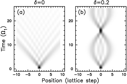
Figure 2: The gray-level plots show the temporal evolution of the probability of presence of the atom, initially localized in the site $m=0$. Plot (a) shows the resonant behavior: the wave packet spreads linearly with time. Plot (b) displays the non-resonant “breathing” behavior. ($\delta$ is indicated in units of $4\Omega_{1}$).

5 Wave packet dynamics

The dynamics of a wave packet can be characterized by calculating mean values of observables. This can be done analytically in the present framework. One can easily deduce from Eq. (4) the mean position:

$$\langle x\rangle_{t}=\sum_{n}X_{nn}\left|d_{n}(t)\right|^{2}+X_{1}\sum_{n}\left(d_{n}(t)^{\ast}d_{n+1}(t)e^{i\phi(t)}+c.c.\right)$$ (21)

where $\phi(t)=\phi_{1}(t)-\phi_{0}(t)=-\omega_{B}t-(F/\omega)\cos(\omega t)$. Using the relation $X_{nn}=X_{00}+n\equiv X_{0}+n$, a straightforward although somewhat lengthy calculation (see Appendix B) produces:

$$\langle x\rangle_{t} = \langle x\rangle_{t=0}+\left\{\left[-\frac{Q(t)}{2}e^{-i\delta t/2}+X_{1}\left(e^{i\phi(t)}-e^{i\phi(0)}\right)\right]\right.$$ (22)

$$\times \left.\sum_{n}d_{n}^{\ast}(0)d_{n+1}(0)+c.c\right\}.$$

The mean position will evolve with time only if the initial packet displays site-to-site quantum coherence, i.e. if $\sum_{n}d_{n}^{\ast}(0)d_{n+1}(0)\neq 0$ (this is also a condition for observing Bloch oscillations, as pointed out in Sec. 2). The evolution in time may display both a fast oscillation at the frequencies $\omega_{B}$ and $\omega$ (and its harmonics) and of a slow oscillation at the frequency $\delta$. Note that the weight ratio between the slow and the fast component is roughly $\Omega_{1}/(\delta X_{1})$: the slow oscillation is dominant close to resonance.

The meaning of the above result can be more clearly appreciate by considering the simple case in which the initial wave packet spreads over $N$ sites and presents a constant phase difference $e^{ik_{0}}$ from site to site:

$$d_{n}(0)=\frac{e^{ik_{0}n}}{\sqrt{N}}.$$ (23)

Substitution into Eq. (22) leads to:

$$\langle x\rangle_{t} = \langle x\rangle_{t=0}+\left\{-Q(t)\cos(k_{0}-\delta t/2)\right.$$ (24)

$$+ \left.2X_{1}\cos\left[k_{0}-\omega_{B}t-(F_{0}/\omega)\cos(\omega t)\right]\right.$$

$$- \left.2X_{1}\cos\left(k_{0}-F_{0}/\omega\right)\right\}$$

If $\delta=0$:

$$\langle x\rangle_{t}-\langle x\rangle_{t=0} = -2\Omega_{1}\cos(k_{0})t$$ (25)

$$+ 2X_{1}\left(\cos\left[k_{0}-\omega_{B}t-(F_{0}/\omega_{B})\cos(\omega_{B}t)\right]\right.$$

$$- \left.\cos\left(k_{0}-F_{0}/\omega_{B}\right)\right)=v_{g}t+f(t)$$

where $v_{g}=-2\Omega_{1}\cos(k_{0})$ is the group-velocity of the wave packet, and $f(t)$ a purely oscillating function. This result shows that the main features of the resonant dynamics are determined by $k_{0}$. If $k_{0}=\pm\pi/2$ (phase-quadrature from site to site), $v_{g}=0$ and there is no global motion (but there is an oscillation and a spreading of the wave packet). If $k_{0}=\pi$, $v_{g}=2\Omega_{1}$ and the global motion is a climb up along the slope of the potential with the maximum speed $2\Omega_{1}$. In the case $k_{0}=0$, where $v_{g}=-2\Omega_{1}$ the atom climbs down the slope of the potential with a constant maximum speed: there is coherent transfer of energy from the modulation to atom, thanks to the particular phase relation between neighbor sites. Contrary to the motion of a classical particle, the speed $\left|v_{g}\right|$ is independent of the sense of the motion: the wave packet climbs the slope up or down at the same speed.

Let us finally note that the spreading of the wave packet $\left\langle x^{2}\right\rangle_{t}$ can also be obtained analytically. However, this leads to heavier formulas, that the interested reader can find in the Appendix B.

Before closing this section, let us note that other resonant behaviors can be observed for $\omega=q\omega_{B}$ ($q$ integer). From the general expression of Eq. (10), one finds for a coupling between sites of the form ($n\rightarrow n\pm q$), for which the same techniques can be applied. For example, resonant interaction with $\omega=2\omega_{B}$, leads to:

$$\dot{d}_{n}(t)=\Omega_{2}\left[d_{n+2}-d_{n-2}\right]$$ (26)

with $\Omega_{2}=\omega X_{2}J_{1}(F_{0}/\omega)$. Numerical calculations show that $X_{2}\ll X_{1}$. Around this resonance, interesting kinds of coherent dynamics can be observed AP_WannierStark_PRA02 .

6 conclusion

We have developed an analytical approach to the dynamics of a wave packet in static and time-modulated tilted lattices, and provided exact solutions describing the atomic motion. It is worth noting that the present description is, in its principle, independent of the shape of the lattice, provided it presents localized states. It is therefore generalizable to non-sinusoidal lattices.

The major experimental difficulty for observing the effects described in this paper is the creation of the initial atomic coherence. There are various solutions for that. One is to cool the atoms to sub-recoil temperatures, so that their de Broglie wavelength is of the order of a few lattice steps (5-10 lattice steps is typical) Salomon_BlochOsc_PRL96 ; the light potential is then turned on adiabatically. Another way of creating spatial coherence is to start with a Bose-Einstein condensate, whose spatial coherence length is up to hundreds lattice sites Kasevich_BECTiltedLattice_Science98 ; Arimondo_BECBlochOsc_PRL01 . Note that in the latter case the system obeys a nonlinear Schrödinger equation, but the present approach can still be generalized to such case AP_ChaosBEC_ARXIV_03 .

The detection of the coherent dynamics described above is simpler in the momentum space, using velocity-sensitive Raman stimulated transitions Chu_RamanVSel_PRL91 ; Salomon_BlochOsc_PRL96 ; AP_RamanSpectro_PRA02 . The coherent motion of atoms, e.g. when they climb the slope of the modulated potential (Sec. 3), correspond to a speed of about a recoil velocity, i.e 3 mm/s for cesium, which can be easily detectable by Raman stimulated spectroscopy. It would be nice to observe the coherent motion also in the real space. This seems to be very difficult, because the spatial amplitude of the motion is very small, of the order of a few lattice steps, as compared to the atomic cloud which extends over hundreds of lattice wells (for atoms cooled in a Magneto-Optical trap). The coherent dynamics is thus detectable in momentum space, but very hard to see in the real space, at least under usual experimental conditions.

Appendix A Bessel addition theorem

The addition theorem for Bessel functions of integer order states that:

$$\sum_{p}J_{p}(r_{0})e^{-ip\theta_{0}}J_{p+q}(r_{1})e^{i(p+q)\theta_{1}}=J_{q}(Q)e^{iq\Theta}$$ (27)

where $\overrightarrow{Q}=\overrightarrow{r}_{1}-\overrightarrow{r}_{0}\equiv R$ $e^{i\Theta}$, and $\overrightarrow{r_{1}}=r_{1}e^{i\theta_{1}}$, $\overrightarrow{r_{0}}=r_{0}e^{i\theta_{0}}$. For Eq. (19), one sets $r_{0}=\frac{2\Omega_{1}}{\delta}\left[1-\cos(\delta t)\right],$ $\theta_{0}=-\pi/2$ $r_{1}=\frac{2\Omega_{1}}{\delta}\sin(\delta t)$, $\theta_{1}=0$, and finds quite straightforwardly

$$Q = \sqrt{r_{1}^{2}+r_{0}^{2}}$$

$$= \frac{4\Omega_{1}}{\delta}\sin\frac{\delta t}{2}$$

and

$$\Theta=\frac{\delta t}{2}$$

Eq. (10) takes the following form:

$$d(k,t) = d(k,0)\sum_{p,q}J_{p}\left(\frac{2\Omega_{1}}{\delta}\left[1-\cos(\delta t)\right]\right)$$

$$\times J_{p+q}\left(\frac{2\Omega_{1}}{\delta}\sin(\delta t)\right)e^{ip\frac{\pi}{2}}e^{-iqk}$$

$$= d(k,0)\sum_{q}J_{q}\left(Q\right)e^{-iqk}e^{iq\frac{\delta t}{2}}$$

Appendix B Mean values

Consider first the first term on the R.H.S of Eq. (21):

$$\left\langle x\right\rangle_{t}^{(1)} = \sum_{n}(X_{0}+n)\sum_{m}J_{m}(Q)d_{n+m}^{\ast}(0)e^{-im\delta t/2}$$ (28)

$$\times \sum_{\ell}J_{\ell}(Q)d_{n+\ell}(0)e^{i\ell\delta t/2}.$$

Changing variables so that $q=m-\ell$, $p=n+\ell$ leads to:

$$\left\langle x\right\rangle_{t}^{(1)} = \sum_{n,q,\ell}\left(X_{0}+n\right)d_{n+\ell}(0)d_{n+\ell+q}^{\ast}(0)J_{\ell}J_{\ell+q}e^{-iq\delta t/2}$$

$$= \sum_{p,q,\ell}\left(X_{0}+p-\ell\right)d_{p}(0)d_{p+q}^{\ast}(0)J_{\ell}J_{\ell+q}e^{-iq\delta t/2}$$

where $J_{n}\equiv J_{n}\left(Q\right)$, $Q=\frac{4\Omega_{1}}{\delta}\sin(\frac{\delta t}{2})$. Eq. 27 implies here:

$$\sum_{\ell}J_{\ell}(Q)J_{\ell+q}(Q)=J_{q}(0)=\delta_{q,0}.$$ (29)

and using also the Bessel recurrence:

$$\ell J_{\ell}(Q)=\frac{Q}{2}\left(J_{\ell+1}(Q)+J_{\ell-1}(Q)\right)$$ (30)

one gets then

$$\left\langle x\right\rangle_{t}^{(1)} = \sum_{p}\left(X_{0}+p\right)\left|d_{p}(0)\right|^{2}-$$

$$\left(\frac{Q}{2}e^{-i\delta t/2}\sum_{p}d_{p}(0)d_{p+1}^{\ast}(0)+c.c.\right).$$

sub It is simpler to show, by the same kind of reasoning, that the second term in Eq. (21) is

$$\left\langle x\right\rangle_{t}^{(2)} = X_{1}\sum_{p}\left(d_{p}(t)^{\ast}d_{p+1}(t)e^{i\phi(t)}+c.c.\right)$$

$$= X_{1}\sum_{p}\left(d_{p}(0)^{\ast}d_{p+1}(0)e^{i\phi(t)}+c.c.\right),$$

so that the mean is:

$$\left\langle x\right\rangle_{t}=\left\langle x\right\rangle_{t=0} + \left\{\left[-\frac{Q}{2}e^{-i\delta t/2}+X_{1}\left(e^{i\phi(t)}-e^{i\phi(0)}\right)\right]\right.$$

$$\times \left.\left(\sum_{p}d_{p}(0)^{\ast}d_{p+1}(0)\right)+c.c.\right\}$$

with

$$\left\langle x\right\rangle_{t=0} = \sum_{p}\left(X_{0}+p\right)\left|d_{p}(0)\right|^{2}$$

$$+ X_{1}e^{i\phi(0)}\sum_{p}\left(d_{p}(0)^{\ast}d_{p+1}(0)+c.c.\right)$$

.

One can calculate, by the same kind of technique, the spreading of the wave packet:

$$\left\langle x^{2}\right\rangle_{t} = \left\langle x^{2}\right\rangle_{t=0}-Q\sum_{p}\left\{\left[\left(X_{0}+p+\frac{1}{2}\right)e^{-i\delta t/2}\right.\right.$$ (31)

$$+ \left.\left.X_{1}^{(2)}\left(e^{i\phi(t)}-e^{i\phi(0)}\right)\right]d_{p}^{\ast}(0)d_{p+1}(0)+c.c.\right\}$$

$$+ \frac{Q^{2}}{4}\sum_{p}\left[\left(d_{p}^{\ast}(0)d_{p+2}(0)e^{-i\delta t}+\left|d_{p}(0)\right|^{2}+c.c.\right)\right]$$

where $X_{1}^{(2)}=\int\varphi_{0}^{\ast}(x)x^{2}\varphi_{1}(x)$, and

$$\left\langle x^{2}\right\rangle_{t=0} = \sum_{p}\left(X_{0}^{(2)}+2pX_{0}+p^{2}\right)\left|d_{p}(0)\right|^{2}$$

$$+ X_{1}^{(2)}e^{i\phi(0)}\sum_{p}\left(d_{p}(0)^{\ast}d_{p+1}(0)+c.c.\right)$$

with $X_{0}^{(2)}=\int\varphi_{0}^{\ast}(x)x^{2}\varphi_{0}(x)=\int\varphi_{n}^{\ast}(x)x^{2}\varphi_{n}(x)-2nX_{0}-n^{2}$.

References

• (1) F Bloch, Z. Phys. 52, 555 (1928).
• (2) C Zener, Proc. R. Soc. (London) A 145, 523 (1934).
• (3) C Cohen-Tannoudji, Atomic motion in laser ligh in Fundamental Systems in Quantum Optics J. Dalibard, J. M. Raimond, and J. Zinn-Justin, editors, p. 1 North-Holland. Amsterdam (1992).
• (4) P Meystre, Atom Optics, Springer Verlag, New York (2001).
• (5) M Ben Dahan, E Peik, J Reichel, Y Castin, and C Salomon, Phys. Rev. Lett. 76, 4508 (1996)
• (6) O Morsch, J H Mueller, M Cristiani, D Ciampini, and E Arimondo, Phys. Rev. Lett. 87, 140402 (200)1.
• (7) S R Wilkinson, C F Bharucha, K W Madison, Q Niu, and M G Raizen, Phys. Rev. Lett., 76, 4512 (1996).
• (8) B P Anderson and M Kasevich, Science 282, 1686 (1998).
• (9) G H Wannier, Phys. Rev. 117, 432 (1960).
• (10) M Gluck, A R Kolovsky, and H J Korsch, Phys. Rev. Lett. 83, 891 (1999).
• (11) Q Thommen, J C Garreau, and V Zehnlé, Phys. Rev. A 65, 053406 (2002).
• (12) H L Haroutyunyan and G Nienhuis, Phys. Rev. A 64, 033424 (2001).
• (13) E E Mendez, F Agulló-Rueda, and J M Hong, Phys. Rev. Lett. 60, 2426 (1988).
• (14) P Voisin, J Bleuse, C Bouche, S Gaillard, C Alibert, and A Regreny, Phys. Rev. Lett. 61, 1639 (1988).
• (15) M Holthaus, J. Opt. B: Quantum Semiclass. Opt. 2, 589 (2000).
• (16) Q Thommen, J C Garreau, and V Zehnlé, Arxiv quantum-ph/0306172 (2003).
• (17) M Kasevich, D S Weiss, E Riis, K Moler, S Kasapi, and S Chu, Phys. Rev. Lett. 66, 2297 (1991).
• (18) J Ringot, P Szriftgiser, and J C Garreau, Phys. Rev. A 65, 013403 (2002).