Misbelief and misunderstandings on the non–Markovian dynamics of a damped harmonic oscillator

Abstract

We use the exact solution for the damped harmonic oscillator to discuss some relevant aspects of its open dynamics often mislead or misunderstood. We compare two different approximations both referred to as Rotating Wave Approximation. Using a specific example, we clarify some issues related to non–Markovian dynamics, non–Lindblad type dynamics, and positivity of the density matrix.

I Introduction

The theory of open quantum systems deals with the dynamics of quantum systems interacting with their surroundings. The most common approach to the description of the time evolution of the system stems from the fact that the total system, i.e., subsystem plus environment, is closed. Hence the density matrix, containing all the information on the state of the total system, satisfies the Liouville-Von Neumann Master Equation. However, due to the eventual complexity of the total system, this Master Equation usually cannot be solved neither analytically nor numerically. Moreover, the density matrix of the total system often contains much more information than what we actually need, since, by definition, we call ‘system’ that part of the universe which is of interest for our study . In other words, we focus our attention only on the degrees of freedom of the system. Mathematically this corresponds to a trace over the environmental variables leading to the reduced density matrix of the system $\rho_{S}$. The dynamics of $\rho_{S}$ can be rather involved because of the effects of the interaction with the environment. In general, understanding these effects is not an easy task.

In this paper we concentrate on a paradigmatic model of the theory of open systems, namely the damped harmonic oscillator. We consider a single harmonic oscillator interacting with a quantized environment modelled as an infinite chain of non-interacting oscillators. This model, also known as quantum Brownian motion (QBM) model, is central in many physical contexts, e.g., in quantum field theory cohen , quantum optics petruccionebook ; carmichael ; buzeck and solid state physics weiss . The importance of the damped harmonic oscillator model is also due to the fact that it is one of the few non-trivial systems for which an exact Master Equation for the reduced density matrix can be formulated and exactly solved Haake ; Feynman ; Caldeira ; Hu ; Ford ; Grabert ; PRAsolanalitica . For this reason it has been extensively studied both for fundamental and for applicative research. On the one hand, indeed, it allows to gain new insight in the process of decoherence, responsible for the appearance of a classical world from the quantum world giulini . On the other hand, it is the key model for many types of new quantum technologies such as quantum computation steane , quantum cryptography crypt , and quantum teleportation telep .

In this paper we discuss a recent analytic approach PRAsolanalitica aimed at solving the generalized Master Equation describing the reduced system dynamics in very general conditions. The method does not rely, indeed, neither on the Born–Markov approximation, leading to a coarse grained description of the dynamics, nor on the weak coupling assumption, valid for quasi–closed system. We will give an expression of the density matrix easily readable in physical terms since it is simply related to diffusion and dissipation coefficients. Moreover, we will use this analytic method to discuss some points usually mislead. In particular two different approximations both usually (and confusingly) referred to as Rotating Wave Approximation (RWA) will be compared. We give examples clarifying the relationship between the following issues: non–Markovian dynamics, non–Lindblad type dynamics, and the positivity of the density matrix.

The paper is organized as follows. In Sec. I we introduce the generalized Master Equation and its exact solution. In Sec. II we discuss the two types of RWAs and single out a class of observables not sensitive to the presence of rapidly oscillating terms. In Sec. III we study the short time non–Markovian dynamics of the mean energy of the system and show the connection with Lindblad or non–Lindblad type behavior. Finally, in Sec. IV conclusions are presented.

II Exact dynamics

Let us consider a harmonic oscillator of frequency $\omega_{0}$ surrounded by a generic environment. The Hamiltonian $H$ of the total system can be written as follows

$$H=H_{0}+H_{E}+\alpha XE,$$ (1)

where $H_{0}=\omega_{0}\left(P^{2}+X^{2}\right)/2$, $H_{E}$ and $\alpha XE$ are the system, environment and interaction Hamiltonians, respectively, and $\alpha$ is the dimensionless coupling constant. The interaction Hamiltonian considered here has a simple bilinear form with position of the oscillator $X$ and position environmental operator $E$. For the sake of simplicity we have written the previous expressions in terms of dimensionless position and momentum operators and set $\hbar=1$. We denote the density matrix for the oscillator-environment system by $\rho$.

Under the assumptions that: (i) at $t=0$ system and environment are uncorrelated, that is $\rho(0)=\rho_{S}(0)\otimes\rho_{E}(0)$, with $\rho_{E}$ the density matrix of the environment; (ii) the environment is stationary, that is $[H_{E},\rho_{E}(0)]=0$; (iii) the expectation value of the environmental operator $E$ is equal to zero, that is ${\rm Tr_{E}}\left\{E\rho_{E}(0)\right\}=0$ (as for example in the case of a thermal reservoir), one can derive the following master equation for QBM EPJRWA

$$\frac{d\rho_{S}(t)}{dt}=-i\mathbf{H}_{0}^{S}-\Big{[}\Delta(t)(\mathbf{X}^{S})^{2}-\Pi(t)\mathbf{X}^{S}\mathbf{P}^{S}$$

$$-\frac{i}{2}r(t)(\mathbf{X}^{2})^{S}+i\gamma(t)\mathbf{X}^{S}\mathbf{P}^{\Sigma}\Big{]}\rho_{S}(t).$$ (2)

We indicate with $\mathbf{X}^{S(\Sigma)}$ and $\mathbf{P}^{S(\Sigma)}$ the commutator (anticommutator) position and momentum operators respectively, and with $\mathbf{H}_{0}^{S}$ the commutator superoperator relative to the system Hamiltonian. Such a Master Equation, obtained by using the time-convolutionless projection operator technique annals ; timeconv , is the superoperatorial version of the Hu-Paz-Zhang Master Equation Hu . Let us note, first of all, that the Master Equation (2) is local in time, even if non-Markovian. This feature is typical of all the generalized Master Equations derived by using the time-convolutionless projection operator technique petruccionebook ; Breuer99a or equivalent approaches such as the superoperatorial one presented in PRAsolanalitica .

The time dependent coefficients appearing in the Master Equation are defined in terms of the noise and dissipation kernels petruccionebook and contain all the information about the short time system-reservoir correlation. The coefficient $r(t)$ gives rise to a time dependent renormalization of the frequency of the oscillator. In the weak coupling limit one can show that this gives a negligible contribution as far as the reservoir cut-off frequency remains finite petruccionebook . The term proportional to $\gamma(t)$ is a classical damping term while the coefficients $\Delta(t)$ and $\Pi(t)$ are diffusive terms.

The superoperatorial Master Equation (2) can be exactly solved by using specific algebraic properties of the superoperators PRAsolanalitica . The solution for the density matrix of the system is derived in terms of the Quantum Characteristic Function (QCF) $\chi_{t}(x,p)$ at time $t$, defined by

$$\rho_{S}(t)=\frac{1}{2\pi}\int\chi_{t}(x,p)\>e^{-i\left(pX-xP\right)}dxdp.$$ (3)

It is worth noting that one of the advantages of the superoperatorial approach is the relative easiness in calculating the analytic expression for the mean values of observables of interest by using the relations:

$$\langle X^{n}\rangle = (-i)^{n}\left(\frac{\partial^{n}}{\partial p^{n}}\chi(x,p)\right)_{x,p=0},$$

$$\langle P^{n}\rangle = (i)^{n}\left(\frac{\partial^{n}}{\partial x^{n}}\chi(x,p)\right)_{x,p=0}.$$ (4)

Neglecting the frequency renormalization terms, the exact analytic expression for the time evolution of the QCF is PRAsolanalitica

$$\chi_{t}(x,p)=e^{-A_{t}(x,p)}\chi_{0}\left[e^{-\Gamma(t)}\tilde{x},e^{-\Gamma(t)}\tilde{p}\right],$$ (5)

with $\chi_{0}$ QCF of the initial state of the system and

$$\tilde{x} = \cos(\omega_{0}t)x+\sin(\omega_{0}t)p,$$

$$\tilde{p} = -\sin(\omega_{0}t)x+\cos(\omega_{0}t)p.$$ (6)

The quantity $A_{t}(x,p)$ is a quadratic form in the position $x$ and momentum $p$ variables:

$$A_{t}(x,p)=(x,p\,)A(t)\Big{(}\begin{array}[]{c}x\\ p\\ \end{array}\Big{)},$$ (7)

with

$$A(t)=e^{-\Gamma(t)}\int_{0}^{t}e^{\Gamma(t_{1})}R^{{\dagger}}(t,t_{1})M(t)R(t,t_{1})dt_{1}.$$ (8)

In this equation, the matrix $R(t,t_{1})$ contains rapidly oscillating terms and $M(t)$ is given by

$$\left(\begin{array}[]{cc}\Delta(t)&-\Pi(t)/2\\ -\Pi(t)/2&0\\ \end{array}\right),$$ (9)

with $\Delta(t)$ and $\Pi(t)$ diffusion coefficients present in the Master Equation (2). Finally the time dependent term $\Gamma(t)$ appearing in Eqs. (5) and (8) is simply related to the dissipation coefficient $\gamma(t)$:

$$\Gamma(t)=2\int_{0}^{t}\gamma(t_{1})\>dt_{1}.$$ (10)

Eq. (5) shows that the QCF is the product of an exponential factor, depending on both the diffusion coefficients [$\Delta(t)$ and $\Pi(t)$] and the dissipation coefficient [$\gamma(t)$], and a transformed initial QCF. The exponential term accounts for energy dissipation and is independent of the initial state of the system. Information on the initial state is given by the second term of the product, the transformed initial QCF. Note that for long times $\chi_{0}\left[e^{-\Gamma(t)}\tilde{x},e^{-\Gamma(t)}\tilde{p}\right]\rightarrow 1$, and the system approaches, as one would expect, a thermal state at the reservoir temperature, whatever the initial state was.

III Rotating Wave Approximations

In this section we discuss the existence of two approximations often called with the very same name: RWA. Such a situation, of course, may cause misleading and, in some cases, can lead to an inaccurate description of the short time dynamics of a damped harmonic oscillator. A similar analysis on the RWA has been performed by Agarwal for the Master Equation describing spontaneous emission in a two-level system agarwal .

Let us begin discussing what we will call the ‘RWA performed after tracing over the environment’. Such an approximation consists in averaging over the rapidly oscillating terms contained in the matrices $R(t,t_{1})$, appearing in Eq. (8) (for the precise analytical calculation see Ref. PRAsolanalitica ). This approximation can be actually seen as a secular approximation, and therefore to avoid confusion we will call it hereafter with this name. Note that the microscopic interaction Hamiltonian contains the so-called counter–rotating terms not conserving the unperturbed energy of the system and reservoir. The crucial point to stress is that the contribution of these terms is not washed out by the average over the rapidly oscillating terms, as we will show with a specific example later in this section.

The second type of RWA is what we will call ‘RWA performed before tracing over the environment’, or simply the RWA. In this case the counter–rotating terms are already absent in the microscopic system–reservoir interaction Hamiltonian which reads:

$$H_{I}=\sum_{n}\left(g_{n}a^{{\dagger}}b_{n}+h.c.\right),$$ (11)

with $b_{n}$ annihilation operators of the reservoir harmonic oscillators, $a=\left(X+iP\right)/\sqrt{2}$ and $a^{{\dagger}}=\left(X-iP\right)/\sqrt{2}$. This interaction Hamiltonian is very common in Quantum Optics, but does not give an appropriate description of the dynamics for short times, since the virtual processes associated to the counter–rotating terms play an important role even for weak couplings.

To illustrate better this point we consider the short time dynamics of a specific observable for the system: its mean energy $H_{0}=\omega_{0}(n+1/2)$, with $n$ quantum number operator. $H_{0}$ belongs to a class of operators which do not depend on the rapidly oscillating terms averaged in the secular approximation PRAsolanalitica . Hence for calculating the mean value of these operators we can use the simpler secular solution of the density matrix. The expression obtained in this way is exact. It has been shown PRAsolanalitica that a sufficient condition to single out this class of operators is the following

$$\left[(\mathbf{X}^{S})^{2}-(\mathbf{P}^{S})^{2}\right]A=0,\hskip 28.45274pt\mathbf{X}^{S}\mathbf{P}^{S}A=0,$$ (12)

with $A$ generic observable of the system.

Let us now compare the short time expressions of the mean quantum number $n$ of the system obtained after performing the secular and RWA approximations. For simplicity we will consider the case of weak coupling between system and a reservoir at $T$ temperature. It is not difficult to prove that the short time non–Markovian expression of $n(t)$, in the secular approximation, can be written as follows EPJRWA

$$\langle n\rangle(t\ll\omega_{c}^{-1})\rightarrow\left[2\alpha^{2}\int_{0}^{\infty}\omega|g(\omega)|^{2}\left(n(\omega)+\frac{1}{2}\right)d\omega\right]\frac{t^{2}}{2},$$ (13)

where $n(\omega)$ is the mean number of reservoir excitations at $T$ temperature and $g(\omega)$ is the reservoir spectral density with cut-off frequency $\omega_{c}$. For the considerations made earlier, this expression coincides with the exact mean value of $n$ (see also ref. grab ).

A similar calculation shows that, if we perform the ‘RWA before tracing over the environment’, the short time expression of the mean number $\langle n\rangle_{RWA}(t\ll\omega_{c}^{-1})$ is exactly half of $\langle n\rangle(t\ll\omega_{c}^{-1})$ as given by Eq. (13). Such a circumstance can be directly related to the fact that, in second order perturbation theory, the virtual processes due to the counter rotating terms combine to give rise to a real process. Thus, neglecting them, as it is done in Eq. (11), amounts at neglecting one of the two channels through which the system can exchange energy with the environment. For this reason the variation of energy predicted in the RWA is only half of the exact value.

IV Non–Markovian Dynamics

In this section we will exploit the analytic solution presented in Sec. II to clarify some common misbelief related to non–Markovian Master Equations and non–Markovian dynamics. In order to do this we consider again the specific example presented in previous section, that is the dynamics of the mean energy of the system. In view of the considerations made before, we can simplify the discussion concerning the dynamics of this observable by considering the solution of the Master Equation in the secular approximation EPJRWA ; letteranostra :

$$\frac{d\rho_{S}}{dt}= - \frac{\Delta(t)+\gamma(t)}{2}\left[a^{{\dagger}}a\rho_{S}-2a\rho_{S}a^{{\dagger}}+\rho_{S}a^{{\dagger}}a\right]$$ (14)

$$- \frac{\Delta(t)-\gamma(t)}{2}\left[aa^{{\dagger}}\rho_{S}-2a^{{\dagger}}\rho_{S}a+\rho_{S}aa^{{\dagger}}\right].$$

As for Eq. (2), we emphasize that this Master Equation, even if non–Markovian, does not contain reservoir memory kernels usually associated to non–Markovian generalized Master Equations. In other words, Eq. (14), as well as Eq. (2), is local in time. By definition this means that such an equation of motion for the density matrix is characterized by the fact that the time derivative of $\rho_{S}(t)$ only depends on the actual value of $\rho_{S}(t)$. On the contrary, in non-Markovian Master Equations involving memory kernels, the time derivative of $\rho_{S}(t)$ is related to values $\rho_{S}(t^{\prime})$ of the density matrix at times $t^{\prime}<t$. Dealing with a non–Markovian Master Equation local in time is of course an advantage compared to a description involving memory kernels, since the memory effects of the environment are incorporated in the time dependence of the coefficients. However, the locality of the Master Equations (2) and (14) could seem hard to reconcile with the intuitive idea of the effects that a generic environment may produce.

As noticed in Ref. romero , it is the linearity of the microscopic Hamiltonian model for QBM which forces the Master Equation to be local in time. Indeed, as a consequence of the linear microscopic system–reservoir interaction Hamiltonian, the density matrix of the reduced system is the solution of a linear integro-differential equation (containing the memory kernel). The key point is that a function $f(t)$ satisfying a linear integro-differential equation, as the one satisfied by the density matrix, does not depend on its entire history. Its future behavior is uniquely determined by the Cauchy data, i.e., its initial value and the initial value of its derivative. For the case of a damped harmonic oscillator, the non–Markovian features are restricted by linearity to the ‘memory’of the initial time instant romero . For this reason, the time dependent coefficient provide all the memory effects in the evolution of the density matrix. It is worth reminding that, as underlined by Paz and Zurek in leshouches , ‘perturbative Master Equations can always be shown to be local in time’. In the case of the damped harmonic oscillator this is true also for the exact Master Equation leshouches .

Another aspect worth stressing is related to the structure of the Master Equations (2) and its approximated form (14). It is well known that, when the Markovian approximation is performed, the Lindblad theorem ensures that the Master Equation describing the system dynamics can be put in the Lindblad form. In general, neither Eq. (2) nor Eq. (14), both non–Markovian, are (or can be recast) in Lindblad form. A question therefore may arise naturally: should we care about the positivity of the density matrix? The reason why we ask this question is related to Lindblad theorem, ensuring the positivity of a density matrix satisfying a Master Equation of Lindblad form. When the Master Equation is not in the Lindblad form, as it is in our case, there can be situations in which symptoms of unphysical approximations show up. For example, negative eigenvalues of the density matrix may appear. This is for instance the case of the Caldeira–Leggett model when some particular initial conditions, not consistent with the high temperature approximation, are assumed.

In general, however, it is certainly not true that whenever a Master Equation is not of Lindblad form then it does not preserve the positivity of the density matrix. A basic assumption of the theorem is indeed that the reduced system dynamics constitutes a dynamical semigroup petruccionebook . Thus, it can happen that the Master Equation is not in Lindblad form but conserves the positivity of the density matrix, while it violates the semigroup property. This is actually our case, as one can realize from the time dependence of the coefficients of the Master Equations (2) and (14).

Now, let us have a closer look at the approximated Master Equation (14). The form of this equation is similar to the Lindblad form, with the only difference that the coefficients appearing in the Master Equation (14) are time dependent. For the sake of brevity we will denote hereafter this Lindblad–type Master Equation with time dependent coefficients simply as Lindblad–type Master Equation whenever the time dependent coefficients are positive. Note, however, that Lindblad–type Master Equations, contrarily to Master Equations of Lindblad form (having constant coefficients), do not satisfy the semigroup property. The reason why we focus on the positivity of the time dependent coefficients of Eq. (14) is that the dynamics of the system depends crucially on their sign. One can define two different regions of the parameter space, the first one correspondent to the situation in which the Master Equation coefficients are positive (Lindblad type region) and the second one correspondent to the case in which the coefficients acquire, at some time instants, negative values (non–Lindblad type region). In Ref. inprep a detailed study of the border between the Lindblad and non–Lindlad type regions is carried out and the reservoir parameters governing the passage from one region to the other one are singled out.

The first and important property distinguishing the Lindblad from the non–Lindblad type regions is that in the first one, i.e. whenever the time dependent coefficients of the Master Equation are positive, one may use the ‘standard’Monte Carlo wave function method to unravel Eq. (14) MCWF , and therefore to simulate the system dynamics. Such method is usually used to study numerically the time evolution of Markovian systems since, in order to apply it, one needs to cast the Master Equation in the Lindblad form. Here we note that also when the Markovian approximation is not performed, if the Master Equation is of Lindblad type, the method can be applied. This is, for instance, the case of a damped harmonic oscillator interacting with a high temperature reservoir, as far as the reservoir cut-off frequency is bigger than the frequency of the system oscillator letteranostra . We note that up to recently, only quantum state diffusion unravelings were used for simulating the temporal behavior of a harmonic oscillator interacting with a non-Markovian quantized environment QSD .

We now proceed to illustrate an example showing the short time dynamics of the system in the non–Lindblad type region, that is when the time dependent coefficients of the Master Equation are negative. To this aim we consider the case of the mean energy of the system oscillator when it interacts with an artificially engineered out of resonance reservoir. In order to study this example we first write down the density matrix solution in the secular approximation.

This approximation washes out the contribution of the diffusive term $\Pi(t)$ in Eq. (8), which becomes PRAsolanalitica

$$A(t)=e^{-\Gamma(t)}\int_{0}^{t}e^{\Gamma(t_{1})}\Delta(t_{1})dt_{1}\equiv\Delta_{\Gamma}(t).$$ (15)

The simplified QCF thus reads

$$\chi_{t}(x,p)=e^{-\Delta_{\Gamma}(t)(x^{2}+p^{2})/2}\chi_{0}\left[e^{-\Gamma(t)}\tilde{x},e^{-\Gamma(t)}\tilde{p}\right].$$ (16)

By using Eq. (4) one derives the following expression for the mean energy of the system PRAsolanalitica

$$\langle H_{0}(t)\rangle=e^{-\Gamma(t)}\langle H_{0}(t=0)\rangle+\omega_{0}\Delta_{\Gamma}(t).$$ (17)

Let us now consider the case in which the system oscillator is in its ground state, and the environment is in a thermal state at $T$ temperature. We assume a Ohmic reservoir spectral density with Lorentz-Drude cut–off $\omega_{c}$. Moreover, we consider the case in which $\omega_{c}<\omega_{0}$, that is the spectrum of the reservoir do not completely overlap with the frequency of the system oscillator. This is of course never the case in presence of a natural reservoir. However, it has been recently shown that for quasi–closed systems, as single trapped ions, it is possible to engineer different types of artificial reservoirs, and couple them in a controlled way to the ion motion engineerNIST .

Under the conditions stated above, for high reservoir temperature, the time dependent coefficient $\Delta(t)-\gamma(t)$ shows an oscillatory behavior as depicted in Fig. 1. As one can see from this figure there exist intervals of time in correspondence of which $\Delta(t)-\gamma(t)$ becomes negative. Hence, in general, the Master Equation (14) is not of Lindblad–type. The density matrix, however, is always positive and it is the semigroup property which is clearly violated, as one can see from Fig. 2 where the time evolution of the mean quantum number operator $\langle n\rangle$ (heating function) is plotted. The signature of the non–Lindblad type dynamics of the reduced system is given by the presence of oscillations in its mean energy. These oscillations are due to virtual exchanges of energy between the system and the reservoir. As we have shown in references EPJRWA and  inprep , these virtual processes are absent whenever the Master Equation (14) is of Lindblad–type.

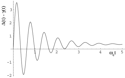
Figure 1: Short time behavior of the time dependent coefficient $\Delta(t)-\gamma(t)$ for $\alpha\omega_{0}=0.1$Hz, $\omega_{0}=10^{7}$Hz, $r=0.1$, and $T=300$K.

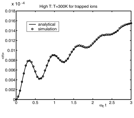
Figure 2: Short time behavior of the heating function for dimensionless coupling constant $\alpha\omega_{0}=0.1$Hz, $\omega_{0}=10^{7}$Hz, $r=0.1$, and $T=300$K. We compare the analytic solution and the Monte Carlo simulation with $10^{7}$ histories.

In Figure 2 the analytic result given by Eq. (17) is compared with the simulation using the Non–Markovian Monte Carlo method Breuer99a ; petruccionebook . In this case indeed, as we have previously discussed, the ‘standard ’Monte Carlo wave function method cannot be applied.

V Conclusions

In this paper we have used the exact solution of a damped harmonic oscillator PRAsolanalitica to discuss some relevant issues of open system dynamics often leading to confusion and/or misunderstandings.

We have focussed our attention on the so called RWA and we have pointed out the existence of two different approximations called with the very same name. In other words we have stressed the differences in what we call the ‘RWA performed before or after tracing over the environment’. The RWA performed before tracing over the environment consists in neglecting the counter–rotating terms in the microscopic Hamiltonian describing the coupling between system and environment. The RWA performed after tracing over the environment is more precisely a secular approximation, consisting in an average over rapidly oscillating terms, but does not wash out the effect of the counter–rotating terms present in the coupling Hamiltonian. By considering a specific example we show how, in the short time non–Markovian regime, the virtual processes due to the counter–rotating terms (neglected in the RWA) give a significant contribution even for weak coupling, and thus need to be taken into account.

We have pointed out that non-Markovian Master Equations do not necessarily contain memory kernels. This concept, already claimed by many authors (see for example petruccionebook ; leshouches ) is still - surprisingly - often seen in a rather sceptical way. We have also discussed a related point which often rises doubts: the conservation of the positivity of the density matrix when the Master Equation ruling its dynamics is not in Lindblad form.

In order to study the dynamical properties of non–Markovian Master Equations, we have introduced two subclasses of Master Equations which are not in the Lindblad form: the Lindblad and non–Lindblad type, and we have stressed their difference. We have presented a new example showing that there exist conditions under which the short time dynamics of a damped oscillator is governed by a non–Lindblad type Master Equation whose solution is always positive. In this case the semigroup property for the reduced dynamics which is violated, and the non Lindblad–type dynamics shows up in the existence of virtual energy exchanges between system and reservoir.

We think that this paper contributes in clarifying some aspects, often mislead, of the non–Markovian dynamics of a damped harmonic. This is important also because very recently the potential interest in non–Markovian reservoirs for quantum information processing has been demonstrated Ahn and a non–Markovian description of quantum computing, showing the limits of the Markovian approach, has been presented horo .

VI Acknowledgements

J.P. acknowledges financial support from the Academy of Finland (project no. 50314), the Finnish IT-Center for Science (CSC) for the computer resources, the University of Palermo for the hospitality, and Kalle-Antti Suominen for the discussions. S.M. acknowledges Finanziamento Progetto Giovani Ricercatori anno 1999, Comitato 02 for financial support.

References

- (1) C. Cohen-Tannoudj, J. Dupont-Roc, and G. Grynberg, Atom-Photon Interactions (John Wiley and sons, 1992).
- (2) H.-P. Breuer and F. Petruccione, The Theory of Open Quantum systems (Oxford University Press, 2002).
- (3) H. J. Carmichael, An Open System Approach to Quantum Optics (Springer-Verlag, Berlin, 1993).
- (4) V. Bužeck and P. L. Knight in Progress in Optics XXXIV (Elsevier, Amsterdam,1995).
- (5) U. Weiss, Quantum Dissipative Systems, 2nd edition (World Scientific, Singapore, 1999).
- (6) F. Haake and R. Reibold, Phys. Rev. A 32, 2462 (1985).
- (7) R. P. Feynman and F. L. Vernon, Ann. Phys. 24, 118 (1963).
- (8) A. O. Caldeira and A. J. Leggett, Physica A 121, 587 (1983).
- (9) B. L. Hu, J. P. Paz, and Y. Zhang, Phys. Rev. D 45, 2843 (1992).
- (10) G.W. Ford and R.F. O’Connell, Phys. Rev. D 64, 105020 (2001).
- (11) H. Grabert, P. Schramm, and G.-L. Ingold, Phys. Rep. 168, 115 (1988).
- (12) F. Intravaia, S. Maniscalco, and A. Messina, Phys. Rev. A 67, 042108 (2003).
- (13) D. Giulini, E. Joos, C. Kiefer, J. Kupsch, I.-O. Stamatescu, and H.-D. Zeh, Decoherence and the Appearence of a Classical World in Quantum Theory (Springer-Verlag, Berlin, 1996).
- (14) A. Steane, Rep. Prog. Phys. 61, 117 (1998).
- (15) N. Gisin, G. Ribordy, W. Tittel, and H. Zbinden, Rev. Mod. Phys. 74, 145 (2002).
- (16) I. Marcikic et al., Nature 421, 509 (2003).
- (17) G.S. Agarwal Springer Tracts in Modern Physics vol. 70, Quantum Optics (Springer-Verlag, Berlin, 1974).
- (18) F. Intravaia, S. Maniscalco and A. Messina, Eur. Phys. J. B, 32, 97 (2003).
- (19) H.-P. Breuer, B. Kappler, and F. Petruccione, Ann. Phys. 291, 36 (2001).
- (20) S. Chaturvedi and J. Shibata, Z. Phys. B 35, 297 (1979); N.H.F. Sgibata and Y. Takahashi, J. Stat. Phys. 17, 171 (1977).
- (21) H. P. Breuer, B. Kappler, and F. Petruccione, Phys. Rev. A 59, 1633 (1999).
- (22) R. Karrlein and H. Grabert, Phys. Rev. E 55, 153 (1997).
- (23) F. Intravaia, S. Maniscalco, J. Piilo, and A. Messina, Phys. Lett. A, 308, (2003).
- (24) L. D. Romero and J. P. Paz, Phys. Rev. A 55, 4070 (1997).
- (25) J. P. Paz and W. H. Zurek in Proceedings of the 72nd Les Houches summer school: Coherent atomic matter waves, R. Kaiser, C. Westbrook and F. David Eds. (Springer-Verlag, 1999).
- (26) J. Dalibard, Y. Castin, and K. Mølmer, Phys. Rev. Lett. 68, 580 (1992); M.B. Plenio and P.L. Knight, Rev. Mod. Phys. 70, 101 (1998).
- (27) W. T. Strunz, L. Diósi, N. Gisin, and T. Yu, Phys. Rev. Lett. 83, 4909 (1999).
- (28) S. Maniscalco, J. Piilo, F. Intravaia, F. Petruccione, H.-P. Breuer, and A. Messina, in preparation.
- (29) C. J. Myatt et al., Nature 403, 269 (2000); Q. A. Turchette et al., Phys. Rev. A 62, 053807 (2000).
- (30) D. Ahn, J. Lee, M. S. Kim and S. W. Hwang, Phys. Rev. A, 66, 012302, (2002).
- (31) R. Alicki, M. Horodecki, P. Horodecki and R. Horodecki, Phys. Rev. A 65, 062101 (2002).