Quantum Kalman Filtering and the Heisenberg Limit in Atomic Magnetometry

Abstract

The shotnoise detection limit in current high-precision magnetometry Kominis et al. (2003) is a manifestation of quantum fluctuations that scale as $1/\sqrt{N}$ in an ensemble of $N$ atoms. Here, we develop a procedure that combines continuous measurement and quantum Kalman filtering Belavkin (1999) to surpass this conventional limit by exploiting conditional spin-squeezing to achieve $1/N$ field sensitivity. Our analysis demonstrates the importance of optimal estimation for high bandwidth precision magnetometry at the Heisenberg limit and also identifies an approximate estimator based on linear regression.

Magnetometry is fundamentally a parameter estimation process because, like all fields, magnetism cannot be directly observed. Rather, the strength of a magnetic field must be inferred from its influence on a probe such as an atomic spin ensemble Dupont-Roc et al. (1969). In a canonical atomic magnetometer, such an ensemble would be prepared into a coherent spin state with its bulk magnetization polarized along the $x$-axis, $\langle\hat{\mathbf{J}}(0)\rangle=(J,0,0)$ (such as by optical pumping). Then, a magnetic field along the $y$-axis with magnitude, $B$, would induce the atomic Bloch vector, $\langle\hat{\mathbf{J}}(t)\rangle$, to precess in the $xz$-plane with frequency, $\omega_{\mathrm{L}}=\gamma B$. Thus, the magnetic field could be estimated from the free induction decay of the atomic magnetization by monitoring the $z$-component of the Bloch vector, $\langle\hat{J}_{\mathrm{z}}(t)\rangle=J\exp(-t/T_{2})\sin(\omega_{\mathrm{L}}t)$, where $T_{2}$ is the transverse spin coherence time.

In practice, current atomic magnetometers operate by continuously pumping the atomic sample while a $\langle\hat{J}_{\mathrm{z}}\rangle$-dependent optical property of the ensemble is monitored Kominis et al. (2003); Budker et al. (2002); Kim and Lee (1998). Due to pumping, the atoms are constantly re-polarized as they Larmor precess. For small fields (the relevant case when discussing detection limits), the ensemble rapidly achieves an equilibrium that is nearly polarized along the $x$-axis, but with a steady-state offset, $\langle\hat{J}_{\mathrm{z}}\rangle_{\mathrm{ss}}\propto\gamma BJ$. The uncertainty in measuring $\hat{J}_{\mathrm{z}}$, is due to projection noise Itano et al. (1993), $\langle\Delta\hat{J}_{\mathrm{z}}^{2}\rangle\equiv\langle\hat{J}_{\mathrm{z}}^{2}\rangle-\langle\hat{J}_{\mathrm{z}}\rangle^{2}$, which has a value of $J/2$ for a coherent spin state. Averaging a sequence of independent measurements of $\langle\hat{J}_{\mathrm{z}}\rangle_{\mathrm{ss}}$ with this variance leads to the conventional shotnoise detection limit for a total measurement time of $t_{\mathrm{tot}}$ Kominis et al. (2003); Budker et al. (2002),

$$\delta B\simeq\frac{1}{\gamma\sqrt{JT_{2}t_{\mathrm{tot}}}}\,.$$ (1)

Since $\langle\Delta\hat{J}_{\mathrm{z}}^{2}\rangle$ sets an intrinsic limit on the field sensitivity, reducing the projection noise below its standard quantum limit would improve the precision. This naturally leads one to consider spin-squeezed states Kitagawa and Ueda (1993) where uncertainty in $\langle\hat{J}_{\mathrm{z}}\rangle$ is reduced by redistributing it into the orthogonal spin component so that $\langle\Delta\hat{J}_{\mathrm{y}}^{2}\rangle>J/2$. Since $\langle\hat{J}_{\mathrm{y}}\rangle$ does not directly affect the field estimation, spin-squeezing should enable one to surpass the conventional shotnoise magnetometry limit.

An improved magnetometry protocol would ideally be implemented by utilizing the conditional spin-squeezing that is automatically generated by continuous observation of an atomic sample Takahashi et al. (1999); Kuzmich et al. (2000); Thomsen et al. (2002). This dynamically generated squeezing does not occur in steady-state (narrow-band) magnetometers because of the continuous optical pumping. However, it should be possible to enable sub-shotnoise magnetometry by turning off the optical pumping once a coherent spin state has been prepared followed by continuous observation of the atoms.

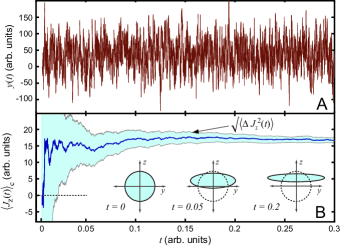
Figure 1: (A) Simulatedsingle-shot atomic magnetometry photocurrent low pass filtered at $F_{\mathrm{c}}=2\pi\sqrt{J}/t_{\mathrm{tot}}$. (B) Corresponding diffusion of the atomic Bloch vector as conditional squeezing is produced by continuous QND observation.

But the nature of conditional spin-squeezing gives rise to potential complications that make it initially unclear how to exploit the reduced uncertainty for improved magnetometry. Fig. 1 shows simulated data (generated according to a quantum trajectory model described below) of a spin ensemble under continuous measurement with no external field, $B=0$. As $\langle\Delta\hat{J}_{\mathrm{z}}^{2}\rangle$ decreases [shaded region in Fig. 1(B)] with the onset of spin-squeezing, there is no apparent change in the noise of the associated $\langle\hat{J}_{\mathrm{z}}(t)\rangle$ measurement, $y(t)$ [Fig. 1(A)], which is due to constant optical shotnoise.

The dynamical generation of spin-squeezing starting from an initial coherent state involves a stochastic transient at early times. As suggested by the error-ellipse diagrams of Fig. 1(B), conditional evolution gradually localizes the quantum spin state around a constant, but random, value of $\langle\hat{J}_{\mathrm{z}}\rangle_{\mathrm{c}}$. In an ensemble of continuous measurement trajectories, this constant value would be distributed with a variance of $J/2$ corresponding to $\langle\Delta\hat{J}_{\mathrm{z}}^{2}\rangle$ of the initial coherent state. Therefore, the mean value of $\langle\hat{J}_{\mathrm{z}}\rangle_{\mathrm{c}}$ assumes a non-zero value even in the absence of an applied magnetic field, producing a stochastic offset in the photocurrent that must be distinguished from Larmor precession in a magnetometry experiment.

Fortunately, with appropriate filtering, Larmor precession of the spin state can be distinguished from the projection noise in such a way that the field estimation benefits from spin-squeezing. In this Letter, we demonstrate that quantum trajectory theory Carmichael (1993); Wiseman and Milburn (1994) allows one to construct a Kalman filter Belavkin (1999); Mabuchi (1996); Verstraete et al. (2001); Stockton et al. (2003) that optimally estimates the field magnitude from continuously observed conditional atomic dynamics. This filtering procedure enables Heisenberg limited magnetometry despite the optical shotnoise and the transient effects of spin state estimation. Furthermore, we show that for time-invariant fields, our optimal strategy approximately reduces to the simple and intuitive data analysis procedure of linear regression which is a potentially simpler experimental approach to sub-shotnoise magnetometry.

We propose a magnetometer in which the atomic ensemble undergoes a continuous quantum non-demolition (QND) observation of $\hat{J}_{\mathrm{z}}$. It has been shown that such a measurement can be implemented by detecting $\hat{J}_{\mathrm{z}}$-dependent changes in the phase of an off-resonant cavity mode coupled to the atomic ensemble Thomsen et al. (2002) or by the Faraday rotation of a far-detuned travelling mode Silberfarb and Deutsch (2003); Smith et al. (2003) that passes through the ensemble. In both cases the magnetometer photocurrent is given by,

$$y(t)\,dt=2\eta\sqrt{M}\langle\hat{J}_{\mathrm{z}}(t)\rangle_{\mathrm{c}}\,dt+\sqrt{\eta}dW(t)\,$$ (2)

where $\langle\hat{J}_{\mathrm{z}}(t)\rangle_{c}$ is the conditional expectation value of $\hat{J}_{\mathrm{z}}$, $\eta$ is the detector efficiency and $M$ (in units of frequency) is an implementation-dependent constant referred to as the measurement strength. The optical shotnoise is reflected by stochastic increments, $dW(t)$, that obey Gaussian white-noise statistics, $E[dW]=0$ and $dW^{2}=dt$.

Conditional evolution of the atomic ensemble subjected to a magnetic field along the $y$-axis and a QND measurement of $\hat{J}_{\mathrm{z}}$ is described by the stochastic master equation,

$$d\hat{\rho}_{c}(t) = -i\gamma B[\hat{J}_{\mathrm{z}},\hat{\rho}_{c}]dt+M\mathcal{D}[\hat{J}_{\mathrm{z}}]\hat{\rho}_{c}dt$$

$$+\sqrt{M\eta}\mathcal{H}[\hat{J}_{\mathrm{z}}]\hat{\rho}_{c}dW(t)$$

where $\hat{\rho}_{c}(t)$ is the reduced atomic density operator conditioned on the measurement record Wiseman and Milburn (1994). The super-operators, $\mathcal{D}$ and $\mathcal{H}$, are given by, $\mathcal{D}[r]\hat{\rho}=r\hat{\rho}r^{\dagger}-(r^{\dagger}r\hat{\rho}+\hat{\rho}r^{\dagger}r)/2$ and $\mathcal{H}[r]\hat{\rho}=r\hat{\rho}+\hat{\rho}r^{\dagger}-\mathrm{tr}[(r+r^{\dagger})\hat{\rho}]\hat{\rho}$, and the initial condition is an optically-pumped coherent spin state along the $x$-axis, $\hat{\rho}(0)=|J\rangle_{x}\langle J|$.

Each term in Eq. (Quantum Kalman Filtering and the Heisenberg Limit in Atomic Magnetometry) has a physical implication for magnetometry. First, the Hamiltonian, $H(B)=\gamma B\hat{J}_{y}$, generates the desired Larmor precession signal used to detect the magnetic field. The second term reflects measurement induced atomic decoherence that results from coupling the ensemble to the optical shotnoise on the probe laser. As a result the length of the Bloch vector decays over time, $J(t)=J\exp(-Mt/2)$, and $M$ can be related to a bound on the transverse spin relaxation, $T_{2}\leq 2M^{-1}$.

The significance of the third term in Eq. (Quantum Kalman Filtering and the Heisenberg Limit in Atomic Magnetometry) is best seen after employing an approximation that holds for a large net magnetization and small field ($\omega_{L}t\ll 1$). For an ensemble polarized along the $x$-axis, quantum fluctuations in $\hat{J}_{x}$ are at least second order and the operator, $\hat{J}_{x}$, is well-approximated by the length of the Bloch vector, $\hat{J}_{x}\rightarrow J$. Physically, this assumption capitalizes on the large value of $J$ to treat the Bloch sphere as a locally flat phase space. This approximation is extremely good for both coherent and squeezed states with $J\gg 1$. In a Gaussian approximation, the first and second moments of $\hat{J}_{\mathrm{z}}$ are sufficient to completely characterize the atomic state. Therefore, equations of motion for the mean and variance,

$$d\langle\hat{J}_{\mathrm{z}}\rangle_{c} = \gamma BJe^{-Mt/2}\,dt+2\sqrt{M\eta}\langle\Delta\hat{J}_{\mathrm{z}}^{2}\rangle\,dW(t)\,\,\,\,$$ (4)

$$d\langle\Delta\hat{J}_{\mathrm{z}}^{2}\rangle = -4M\eta\langle\Delta\hat{J}_{\mathrm{z}}^{2}\rangle^{2}\,dt\vspace{-.2cm}$$ (5)

provide a closed representation of the magnetometer’s conditional quantum dynamics (in the $\omega_{L}t\ll 1$ and $t\lesssim M^{-1}$ limits). The physical significance of Eq. (4) is that the atomic Bloch vector experiences two types of motion: deterministic Larmor precession and stochastic diffusion. Equation (5) reflects the deterministic reduction of $\langle\Delta\hat{J}_{\mathrm{z}}^{2}\rangle$ as the atomic state is localized by the observation process, i.e., conditional spin-squeezing.

Equations (4) and (5) can be used to implement an optimal estimation procedure that capitalizes on squeezing without mistaking measurement-induced Bloch vector rotations for true Larmor precession. Since the atomic dynamics are stochastic, the estimator must be described probabilistically—we desire a conditional probability distribution, $p\left(B|\Xi_{[0,t]}\right)$, which measures the likelihood that the field has magnitude $B$ given the measurement record, $\Xi$, defined in terms of the photocurrent, $d\,\Xi_{\,t}\equiv y(t)\,dt/(2\eta\sqrt{M})$. The estimated magnitude, $\tilde{B}$, and its uncertainty, $\Delta\tilde{B}^{2}$ are obtained from the moments,

$$\tilde{B} = \int Bp\left(B|\Xi_{[0,t]}\right)\,dB$$ (6)

$$\Delta\tilde{B}^{2} = \int(B-\tilde{B})^{2}p\left(B|\Xi_{[0,t]}\right)\,dB$$ (7)

of the conditional distribution, $p\left(B|\Xi_{[0,t]}\right)$.

Constructing a maximum-likelihood estimator is accomplished by defining an update rule that iteratively improves $p\left(B|\Xi_{[0,t]}\right)$ as the measurement record is acquired. Prior knowledge of the distribution of magnetic field values is encoded in $p\left(B|\Xi_{0}\right)$, which may be assigned infinite variance in order to assure an unbiased estimate. Optimality requires that the conditional probability must be updated according to a Bayes’ rule,

$$dp\big{(}B|d\,\Xi_{\,t},\Xi_{[0,t)}\big{)}=dq\big{(}d\,\Xi_{\,t}|B,\Xi_{[0,t)}\big{)}p\big{(}B|\Xi_{[0,t)}\big{)}$$ (8)

where $dq\big{(}d\,\Xi_{\,t}|B,\Xi_{[0,t)}\big{)}$ is an infinitesimal conditional probability that describes the likelihood of the evolving measurement record, $d\,\Xi_{\,t}$, given a field with magnitude $B$ and past history, $\Xi_{[0,t)}$. The utility of Bayes’ rule is that $q\big{(}d\,\Xi_{\,t}|B,\Xi_{[0,t)}\big{)}$ can be computed using quantum trajectory theory, Eqs. (4) and (5).

Implementing this parameter estimator is best accomplished by a (recursive) Kalman filter Belavkin (1999); Mabuchi (1996); Verstraete et al. (2001). It can be shown that the filtering equations,

$$d\tilde{x}=\mathbf{A}\tilde{x}\,dt+D^{-2}(\mathbf{B}+\mathbf{VC}^{T})(d\,\Xi-\mathbf{C}\tilde{x}\,dt)$$ (9)

with $\tilde{x}\equiv\left(\begin{array}[]{cc}\tilde{J}_{\mathrm{z}}&\tilde{B}\\ \end{array}\right)^{T}$, ($\tilde{J}_{\mathrm{z}}$ is the estimate of $\langle\hat{J}_{\mathrm{z}}\rangle_{c}$),

$$\mathbf{A}=\gamma Je^{\frac{-Mt}{2}}\left(\begin{array}[]{cc}0&1\\ 0&0\\ \end{array}\right),\,\,\,\mathbf{B}=\left(\begin{array}[]{c}\langle\Delta\hat{J}_{\mathrm{z}}^{2}\rangle\\ 0\end{array}\right),\,\,\,\mathbf{C}=\left(\begin{array}[]{cc}1&0\\ \end{array}\right),$$

$D=1/(2\sqrt{M\eta})$, and $\tilde{x}(0)=0$ implement Eq. (8). We note that it is possible to extend the Kalman filter to account for time-varying or stochastic fields Stockton et al. (2003) as well as to implement quantum feedback control Stockton et al. (2003); Thomsen et al. (2002).

The conditional quantum dynamics, particularly spin-squeezing and the exponential decay of the Bloch vector, enter the estimation process via the covariance matrix,

$$\mathbf{V}(t)=\left(\begin{array}[]{cc}\Delta\tilde{J}_{\mathrm{z}}^{2}(t)&\Delta(\tilde{J}_{\mathrm{z}}\tilde{B})(t)\\ \Delta(\tilde{B}\tilde{J}_{\mathrm{z}})(t)&\Delta\tilde{B}^{2}(t)\\ \end{array}\right)$$ (10)

which describes the uncertainty in the parameter estimations of $\hat{J}_{\mathrm{z}}$ and $B$. $\mathbf{V}(t)$ evolves deterministically according to the matrix Riccati equation,

$$\dot{\mathbf{V}} = \left(\mathbf{A}-D^{-2}\mathbf{BC}\right)\mathbf{V}+\mathbf{V}\left(\mathbf{A}-D^{-2}\mathbf{BC}\right)^{T}$$

$$\,+\,D^{-2}\mathbf{V}\left(\mathbf{C}^{T}\mathbf{C}\right)\mathbf{V}$$

subject to the initial conditions $\Delta\tilde{J}_{\mathrm{z}}^{2}(0)=0$ and $\Delta(\tilde{J}_{\mathrm{z}}\tilde{B})(0)=0$, with $\Delta\tilde{B}^{2}(0)$ chosen to reflect prior knowledge on the distribution of magnetic field values. Lacking any such knowledge, one can set $\Delta\tilde{B}^{2}(0)\to\infty$.

The smallest detectable magnetic field as a function of $J$ and the measurement duration, $t$, is determined by the estimator variance, $\Delta\tilde{B}^{2}$. Solving the the matrix Riccati equation [which is analytically soluble for the Kalman filter in Eq. (9)], provides the time-dependent magnetic field detection threshold, $\delta\tilde{B}\equiv\sqrt{\Delta\tilde{B}^{2}(t)}$,

$$\delta\tilde{B}(t)=\frac{M}{4\gamma J}\sqrt{\frac{(1+2\eta JMt)}{ae^{-Mt}+4e^{-Mt/2}(4\eta J+1)+b}}$$ (12)

with $a$ and $b$ given by,

$$a = -(2\eta J(Mt+4)+1)$$

$$b = Mt+2\eta J(Mt-4)-3\,\,.$$

Expanding Eq. (12) to leading order in $t$ provides an expression for the detection threshold,

$$\delta\tilde{B}(t)\approx\frac{1}{\gamma J}\sqrt{\frac{3}{M\eta t^{3}}},\quad t\gg(JM)^{-1}.$$ (13)

that is directly comparable to Eq. (1) when the measurement strength is chosen to be $M\sim T_{2}^{-1}$ such that maximal spin-squeezing is achieved at time $t=M^{-1}$. Such a choice for $M$ permits a superior $1/J$ (equivalently $1/N$) scaling that is characteristic of the Heisenberg squeezing limit Kitagawa and Ueda (1993); Thomsen et al. (2002). The optical shotnoise [of order unity in this model, see Eq. (2)] enters implicitly through the signal to noise ratio, SNR=$J\sqrt{M}$, which highlights the utility of the Kalman filter as a whitening filter— it extracts the non-stationary spin-squeezing and Larmor precession dynamics despite the presence of Gaussian noise.

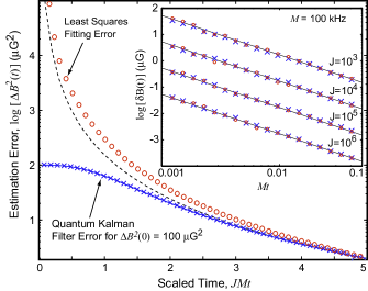
Figure 2: Comparison of the estimation errors for a quantum Kalman filter and a linear least squares magnetic field determination. The inset plot highlights the $1/J$ (Heisenberg limited) scaling of both procedures for $t\gg(JM)^{-1}$.

Figure 2 shows numerical results that demonstrate the performance of our quantum Kalman filter (QKF). The simulations were performed for an atomic ensemble with $J=4\times 10^{6}$, $\gamma=1$ kHz/mG, $\eta=1$, and $M=100$ kHz in a background magnetic field of $B=1$ $\mu$G. These values nearly correspond to a magnetometer constructed from $N=10^{6}$ ground state Cs atoms coupled to a high-finesse optical cavity with single photon Rabi frequency $g_{0}$ = 10 MHz and decay rate, $\kappa$ = 1 MHz. The QND measurement corresponds to a phase-quadrature homodyne detection of the transmitted cavity light with a cavity mode ($P=100$ $\mu$W) that is blue detuned by $\Delta=1$ GHz from the Cs transition at $\lambda\sim 852$ nm. The initial estimator variance was chosen to be $\Delta\tilde{B}^{2}(0)=100$ $\mu$G² which is the initial value that one would select given prior knowledge that the magnetic field could be treated as a Gaussian random variable with this variance. For the parameters we selected, Larmor precession and spin projection noise have comparable magnitudes on timescales of order $(JM)^{-1}$.

The Kalman estimation error (crosses in Fig. 2) was computed from the ensemble average, $E[(\tilde{B}_{i}-B)^{2}]$, for $10^{5}$ trajectories, and the solid line shows the estimation uncertainty $\Delta\tilde{B}(t)$ obtained by integrating Eq. (Quantum Kalman Filtering and the Heisenberg Limit in Atomic Magnetometry). Since our simulations were performed with $B=1$ $\mu$G, the empirical performance of the QKF closely matches the solid line. The dotted line in Fig. 2 shows the analytic Riccati solution, given by Eq. (12), for $\Delta\tilde{B}^{2}(0)\rightarrow\infty$, which would be the expected QKF performance in a scenario with no prior knowledge of the magnetic field. Fig. 2 also shows the estimation error for simple linear regression of the measurement record (open circles). Assuming that the Bloch vector has not decayed significantly, $\tilde{B}$ is proportional to the slope of a line fit to the (filtered) photocurrent, $y(t)$. The estimation error for linear regression was obtained by computing $E[(\tilde{B}_{i}-B)^{2}]$ for $10^{5}$ trajectories. Although the QKF is clearly superior for short times, the two estimation procedures converge for $(JM)^{-1}\ll t<M^{-1}$ and provide a quantum parameter estimation with $\delta\tilde{B}\sim$ 0.01 nG in $t\sim 1$ ms. The inset of Fig. 2 highlights the $\delta\tilde{B}\propto J^{-1}$ scaling that distinguishes both the QKF (crosses) and regression (open circle) estimators from the conventional shot-noise limit, Eq. 1. For sufficiently large times both estimators achieve the detection threshold in Eq. 13 (solid lines).

The QKF and linear regression differ mainly in how they treat the initial diffusive transient of $\hat{J}_{\mathrm{z}}$ [Fig. 1(B)]. Since the QKF is derived from a quantum trajectory model, it is aware of the short-time diffusion and strategically under-weights the photocurrent at early times [via the Kalman gain, $\mathbf{G}\equiv D^{-2}(\mathbf{B}+\mathbf{VC}^{T})$]. At late times the regression analysis manages to absorb the initial diffusive transient into the $y$-intercept of the linear fit. Although $\langle\hat{J}_{\mathrm{z}}(0)\rangle=0$, the $\hat{J}_{\mathrm{z}}$ localization process gradually determines an effective offset in the photocurrent during the interval $t\sim(JM)^{-1}$. Without explicit knowledge of the conditional dynamics the linear regression equally weights the photocurrent for $t<(JM)^{-1}$. This decreases the quality of the fit, but the resulting error becomes insignificant for $t\gg(JM)^{-1}$.

Our analysis suggests that estimation procedures based on conditional quantum dynamics can play a crucial role in optimizing both the sensitivity and the bandwidth in atomic magnetometry. While conventional steady-state magnetometers can only improve their detection capabilities by increasing the number of atoms or the averaging time, the quantum estimator can achieve greater precision for the same value of $t$ and $N$ by improving the measurement strength. The significance of the Kalman filter is the optimality that is guaranteed by its derivation from a Bayes’ rule. Our finding that linear regression closely approximates the optimal procedure indicates a potentially simpler experimental procedure for sub-shotnoise magnetometry. Although Heisenberg limited spin-squeezing should be possible using current techniques in cavity quantum electrodynamics (a discussion is provided in Thomsen et al. (2002)), the experimental difficulty of achieving this limit makes it desirable to have an optimal estimator such as the QKF to fully exploit even a small amount of squeezing, to treat fluctuating fields and to achieve estimator robustness Stockton et al. (2003). In either case, estimation procedures that allow and account for conditional quantum dynamics— whether explicitly as in the QKF or implicitly as in linear regression— offer substantial improvement over steady-state procedures.

This work was supported by the NSF (PHY-9987541, EIA-0086038), the ONR (N00014-00-1-0479), and the Caltech MURI Center for Quantum Networks (DAAD19-00- 1-0374). JKS acknowledges a Hertz fellowship. Please visit http://minty.caltech.edu/Ensemble for simulation source code and detailed notes on the Kalman filter derivation.

References

- Kominis et al. (2003) I. Kominis, T. Kornack, J. Allred, and M. Romalis, Nature 422, 596 (2003).
- Belavkin (1999) V. Belavkin, Rep. on Math. Phys. 43, 405 (1999).
- Dupont-Roc et al. (1969) J. Dupont-Roc, S. Haroche, and C. Cohen-Tannoudji, Phys. Lett. A 28, 638 (1969).
- Budker et al. (2002) D. Budker, W. Gawlik, D. Kimball, S. Rochester, V. Yashchuk, and A. Weiss, Rev. Mod. Phys. 74, 1153 (2002).
- Kim and Lee (1998) C. Kim and H. Lee, Rev. Sci. Inst. 69, 4152 (1998).
- Itano et al. (1993) W. Itano, J. Berquist, J. Bollinger, J. Gilligan, D. Heinzen, F. Moore, M. Raizen, and D.J.Wineland, Phys. Rev. A 47, 3554 (1993).
- Kitagawa and Ueda (1993) M. Kitagawa and M. Ueda, Phys. Rev. A 47, 5138 (1993).
- Takahashi et al. (1999) Y. Takahashi, K. Honda, N. Tanaka, K. Toyoda, K. Ishikawa, and T. Yabuzaki, Phys. Rev. A 60, 4974 (1999).
- Kuzmich et al. (2000) A. Kuzmich, L. Mandel, and N. P. Bigelow, Phys. Rev. Lett. 85, 1594 (2000).
- Thomsen et al. (2002) L. Thomsen, H. Mancini, and H. Wiseman, Phys. Rev. A 65, 061801 (2002).
- Carmichael (1993) H. Carmichael, An open systems approach to quantum optics (Springer-Verlag, New York, 1993).
- Wiseman and Milburn (1994) H. Wiseman and G. Milburn, Phys. Rev. A 49, 1350 (1994).
- Mabuchi (1996) H. Mabuchi, Quantum Semiclass. Opt. 8, 1103 (1996).
- Verstraete et al. (2001) F. Verstraete, A. Doherty, and H. Mabuchi, Phys. Rev. A 64, 032111 (2001).
- Stockton et al. (2003) J. K. Stockton, J. Geremia, A. C. Doherty, and H. Mabuchi, quant-ph/0309101 (2003).
- Silberfarb and Deutsch (2003) A. Silberfarb and I. Deutsch, Phys. Rev. A 68, 013817 (2003).
- Smith et al. (2003) G. A. Smith, S. Chaudhury, and P. S. Jessen, J. Opt. B: Quant. Semiclass. Opt. 5, 323 (2003).