Gaussian Entanglement of Formation

Abstract

We introduce a Gaussian version of the entanglement of formation adapted to bipartite Gaussian states by considering decompositions into pure Gaussian states only. We show that this quantity is an entanglement monotone under Gaussian operations and provide a simplified computation for states of arbitrary many modes. For the case of one mode per site the remaining variational problem can be solved analytically. If the considered state is in addition symmetric with respect to interchanging the two modes, we prove additivity of the considered entanglement measure. Moreover, in this case and considering only a single copy, our entanglement measure coincides with the true entanglement of formation.

I Introduction

One of the main novelties of Quantum Information Theory is to consider entanglement no longer merely as an apparent paradoxical feature of correlated quantum systems, but rather as a resource for quantum information processing purposes. This new point of view naturally raises the question regarding the quantification of this resource. How much entanglement is contained in a given state? For pure bipartite states there is, under reasonable assumptions, a simple and unique answer to this question, namely the von Neumann entropy of the reduced state Donald et al. (2002); Vidal (2000); Popescu and Rohrlich (1997). For mixed states there are several entanglement measures Horodecki (2001), which can be distinguished due to their operational meaning and mathematical properties. Such a measure should be non-increasing under mixing as well as under local operations and classical communication (LOCC), and it should return the right value for pure states. The largest measure fulfilling these requirements is the Entanglement of Formation $E_{F}$ Bennett et al. (1996). Operationally, it quantifies the minimal amount of entanglement, which is needed in order to prepare the state by mixing pure entangled states. It is therefore defined as an infimum

$$E_{F}(\rho)=\inf\left\{\sum_{k}p_{k}E(\Psi_{k})\Big{|}\;\rho=\sum_{k}p_{k}|\Psi_{k}\rangle\langle\Psi_{k}|\right\}$$ (1)

over all (possibly continuous) convex decompositions of the state into pure states with respective entanglement $E(\Psi)=S\big{(}{\rm tr}_{B}[|\Psi\rangle\langle\Psi|]\big{)}$, where $S(X)=-{\rm tr}\left[X\log X\right]$ is the von Neumann entropy. By its definition calculating $E_{F}$ is a highly non-trivial optimization problem, which becomes numerically intractable very rapidly if we increase the dimensions of the Hilbert spaces. Remarkably, there exist analytical expressions for two-qubit systems Wootters (1998) as well as for highly symmetric states Terhal and Vollbrecht (2000); Vollbrecht and Werner (2000).

Recently, $E_{F}$ was calculated for the first time for continuous variable states, namely for symmetric Gaussian states of two modes Giedke et al. (2003a). In general, Gaussian states are distinguished among other continuous variable states due to several reasons. Experimentally, they are relatively easy to create and arise naturally as states of the light field of a laser (cf.Vogel et al. (2001)) or in atomic ensembles interacting with light Julsgaard et al. (2000). For this and other reasons they play a more and more important role in Quantum Information Theory (cf. Braunstein and Pati (2003)).

Theoretically, despite the underlying infinite dimensional Hilbert space, they are completely characterized by finitely many quantities – the first and second moments of canonical operators. Moreover, they stand out due to several extremal properties . In fact, the calculation of $E_{F}$ for symmetric two-mode Gaussian states depends crucially on the fact that for given “EPR-correlations” two-mode squeezed Gaussian states are the cheapest regarding entanglement. This implies that in this particular case there is a decomposition in terms of pure Gaussian states, which is optimal for $E_{F}$ in (1).

On the one hand, this raises the question, whether this is generally true for all Gaussian states. On the other hand one may, motivated by the operational interpretation of $E_{F}$, restrict Eq. (1) to decompositions into Gaussian states from the very beginning. After all, Gaussian states arise naturally, whereas the experimental difficulties of preparing an arbitrary pure continuous variable state are by no means simply characterized by the amount of its entanglement. For these reasons we will in the following investigate the Gaussian Entanglement of Formation $E_{G}$ to quantify the entanglement of bipartite Gaussian states by taking the infimum in Eq. (1) only over decompositions into pure Gaussian states.

This article is organized as follows: in Sec. II we recall basic notions concerning Gaussian states. Sec. III defines the Gaussian Entanglement of Formation and provides a major simplification concerning its evaluation for bipartite Gaussian states of arbitrary many modes. In Sec. IV we prove that $E_{G}$ is indeed a (Gaussian) entanglement monotone, in the sense that it is non-increasing under Gaussian local operations and classical communication (GLOCC). The case of general two-mode Gaussian states is solved analytically in Sec. V. The special case of symmetric Gaussian states, for which it was proven in Giedke et al. (2003a) that $E_{G}=E_{F}$ is discussed in detail in Sec. VI, where we give an alternative calculation of $E_{G}$, which is in turn utilized in Sec. VII in order to prove additivity of $E_{G}$ for this particular case. Finally, Sec. VIII applies the measure to some examples which arise when a two-mode squeezed state is sent through optical fibers. The appendix proves a Lemma about decompositions of classical Gaussian probability distributions.

II Gaussian states

Consider a bosonic system of $n$ modes, where each mode is characterized by a pair $Q_{k},P_{k}$ of canonical (position and momentum) operators. If we set $R=(Q_{1},P_{1},\ldots,Q_{n},P_{n})$ the canonical commutation relations are governed by the symplectic matrix

$$\sigma\equiv\bigoplus_{k=1}^{n}\left(\begin{array}[]{cc}0&1\\ -1&0\\ \end{array}\right)$$ (2)

via $[R_{k},R_{l}]=i\sigma_{kl}$. A state is called a Gaussian state if it is completely characterized by the first and second moments of the canonical operators $R_{k}$ in the sense that the corresponding Wigner function is a Gaussian. Utilizing Weyl displacement operators $W_{\xi}\equiv e^{i\xi^{T}\sigma R}$, the first moments $d_{k}\equiv{\rm tr}\left[\rho R_{k}\right]$ can be changed arbitrarily by local unitaries. Hence, all the information about the entanglement of the state is contained in the covariance matrix (CM)

$$\gamma_{kl}\equiv{\rm tr}\left[\rho\{R_{k}-d_{k}{\bf 1},R_{l}-d_{l}{\bf 1}\}_{+}\right],$$ (3)

where $\{\cdot,\cdot\}_{+}$ denotes the anti-commutator. By definition the matrix $\gamma$ is real and symmetric, and due to Heisenberg’s uncertainty relation it has to satisfy $\gamma\geq i\sigma$. For pure Gaussian states we have $\det(\gamma)=1$ or, equivalently, $(\sigma\gamma)^{2}=-{\bf 1}$.

In the following we denote the density operator corresponding to the Gaussian state with covariance matrix $\gamma$ and displacement vector $d$ by $\rho_{(\gamma,d)}$. If the latter is a bipartite state, its tensor product structure corresponds to a partition of the $n$ modes into two subsets.

An important decomposition of $\rho_{(\gamma,0)}$ into pure Gaussian states is given by

$$\rho_{(\gamma,0)}\propto\int d^{2n}\xi\ \rho_{(\gamma_{p},d-\xi)}\ e^{-\frac{1}{4}\xi^{T}(\gamma-\gamma_{p})^{-1}\xi}$$ (4)

where $\gamma_{p}\leq\gamma$ is the covariance matrix of a pure Gaussian state. Since displacements of the form $\rho_{(\gamma,0)}\mapsto\rho_{(\gamma,d)}$ are local operations, Eq. (4) tells us that starting with $\rho_{(\gamma^{\prime},0)}$ we can obtain every Gaussian state with CM $\gamma\geq\gamma^{\prime}$ by means of LOCC operations.

III Gaussian entanglement of formation

We define the Gaussian Entanglement of Formation $E_{G}$ for a bipartite Gaussian state $\rho_{(\gamma,d)}$ by

$$E_{G}\big{(}\rho_{(\gamma,d)}\big{)} \equiv \inf_{\mu}\bigg{\{}\int\mu(d\gamma_{p},dD)\;E(\rho_{(\gamma_{p},D)})\ \Big{|}$$ (6)

$$\quad\rho_{(\gamma,d)}=\int\mu(d\gamma_{p},dD)\rho_{(\gamma_{p},D)}\bigg{\}},$$

where the infimum is taken over all probability measures $\mu$ characterizing convex decompositions of $\rho_{(\gamma,d)}$ into pure Gaussian states $\rho_{(\gamma_{p},D)}$, and $E(\rho_{(\gamma_{p},D)})$ is the von Neumann entropy of the reduced state. For pure $n\times n$ mode Gaussian states this quantity can be readily expressed in terms of the symplectic eigenvalues of the reduced CM. Denote these eigenvalues by $a_{k},k=1,\dots,n$. We have $a_{k}\geq 1$ and define $r_{k}\geq 0$ by $a_{k}=\cosh r_{k}$. Then

$$E(\rho_{(\gamma,d)})=\sum_{k}H(r_{k}),$$ (7)

where

$$H(r)=\cosh^{2}(r)\log_{2}(\cosh^{2}r)-\sinh^{2}(r)\log_{2}(\sinh^{2}r).$$ (8)

To obtain this expression note that any pure $n\times n$ Gaussian state is locally equivalent (via unitary GLOCC) to the tensor product of $n$ two-mode squeezed states with squeezing parameters $r_{k}$ Holevo and Werner (2001). For each tensor factor the entanglement is given by the above formula. Since the symplectic spectrum of the reduced CM is invariant under local unitary GLOCC the $r_{k}$ can be computed directly from $\gamma_{p}$ as described above.

The integrals in Eqs. (6, 6) are taken over the space $\mathbb{R}^{n}$ of displacements and over the set of admissible pure state covariance matrices. The following proposition tells us that it is sufficient to only consider measures $\mu$, which vanish for all but one covariance matrix:

Prop. 1

The Gaussian entanglement of formation for a bipartite Gaussian state $\rho_{(\gamma,d)}$ is given by

$$E_{G}\big{(}\rho_{(\gamma,d)}\big{)}=\inf_{\gamma_{p}}\Big{\{}E(\rho_{(\gamma_{p},0)})\ \big{|}\ \gamma_{p}\leq\gamma\Big{\}},$$ (9)

where the infimum is taken over pure Gaussian states with CM $\gamma_{p}$.

Proof: The proof can be divided into three steps:

(i) The problem can be reformulated in terms of classical Gaussian distributions, by considering Wigner functions instead of density operators. This is formally achieved by taking the trace of the decomposition in Eq. (6) with the phase space displaced parity operator ${\cal P}_{\xi}\equiv W_{\xi}{\cal P}W_{\xi}^{*}$ Grossmann (1976). Then

$${\rm tr}\left[{\cal P}_{\xi}\rho_{(\gamma,d)}\right]=|\gamma|^{-\frac{1}{2}}\exp{\Big{[}-\frac{1}{4}(\sigma\xi+d)^{T}\gamma^{-1}(\sigma\xi+d)\Big{]}}$$ (10)

is up to a normalization factor equal to the Wigner function of $\rho_{(\gamma,d)}$, which in turn completely determines the state.

(ii) All the states $\rho_{(\gamma_{p},D)}$ contributing to Eqs. (6, 6) must have smaller covariance matrices $\gamma_{p}\leq\gamma$, i.e.

$$\mu\bigg{(}\Big{\{}(\gamma_{p},D)\ \big{|}\ \exists_{x}:\langle x,(\gamma-\gamma_{p})x\rangle<0\Big{\}}\bigg{)}=0.$$ (11)

The idea of the proof is that the tails of a Gaussian with CM that is too large would give rise to an increasing and in the end overflowing contribution if we only move far enough away from the center. This is mathematically formalized in Lemma 3 stated and proven in the appendix. To apply Lemma 3 via Eq. (10) to Eq. (6) we need in addition, that the inverse is operator monotone on positive matrices $\gamma>0$.

(iii) Assume that $\tilde{\mu}$ is a measure corresponding to an optimal decomposition of $\rho_{(\gamma,d)}$ giving rise to the infimum in Eq. (6). Then

$$E_{G}(\rho_{(\gamma,d)}) = \int_{\gamma_{p}\leq\gamma}\tilde{\mu}(d\gamma_{p},dD)E(\rho_{(\gamma_{p},D)})$$ (12)

$$\geq \inf_{\gamma_{p}}\Big{\{}E(\rho_{(\gamma_{p},0)})\ \big{|}\ \gamma_{p}\leq\gamma\Big{\}}.$$ (13)

However, by using a Gaussian decomposition of the form in Eq. (4) we know that equality in Eq. (13) can be achieved for a measure $\tilde{\mu}$ which is Gaussian in $D$ and a delta function with respect to $\gamma_{p}$.         

Proposition 1 considerably simplifies the calculation of $E_{G}$, since the optimization is reduced from the set of all possible decompositions to the set of pure states satisfying the matrix inequality $\gamma_{p}\leq\gamma$. Before we proceed to calculate $E_{G}$ analytically for the two-mode case, we will show that $E_{G}$ is indeed a proper entanglement monotone. To confine the argument to CMs (rather than density matrices) we make use of Proposition 1.

IV Monotonicity under Gaussian operations

For $E_{G}$ to serve as a good Gaussian entanglement measure it should not increase under GLOCC. That this is the case is quickly seen using the characterization of Gaussian operations given in Giedke and Cirac (2002); Fiurášek (2002). There it was shown that the change of the CM $\gamma$ of a Gaussian state under Gaussian operations takes the form of a Schur complement:

$$G(\gamma)=\tilde{\Gamma}_{1}-\tilde{\Gamma}_{12}\frac{1}{\tilde{\Gamma}_{2}+\gamma}\tilde{\Gamma}_{12}^{T}\equiv S(\tilde{\Gamma}+0\oplus\gamma).$$ (14)

Here

$$\Gamma=\left(\begin{array}[]{cc}\Gamma_{1}&\Gamma_{12}\\ \Gamma_{12}^{T}&\Gamma_{2}\end{array}\right)$$

is the $4n\times 4n$ CM of the state characterizing the operation $G$ and $\tilde{\Gamma}\geq 0$ is the CM of the partially transposed state .

For positive matrices $A\geq B$ implies $S(A)\geq S(B)$ (cf. (Horn and Johnson, 1987, p.472)). Consequently, if $\gamma\geq\gamma_{p}$, then the transformed CM fulfills $G(\gamma)\geq G(\gamma_{p})$.

Every GLOCC can be decomposed into a pure GLOCC $G_{p}$ mapping pure states onto pure states, and the addition of classical Gaussian noise. This decomposition can easily be shown using the above mentioned ordering of the Schur complements for ordered matrices. The decomposition then reads $G(\gamma_{p})=G_{p}(\gamma_{p})+P$, where the noise is characterized by some positive matrix $P\geq 0$, which is usually state-dependent. Therefore we have $G(\gamma)\geq G(\gamma_{p})\geq G_{p}(\gamma_{p})$ and since the latter CM corresponds to a pure state, which can be obtained from $\gamma_{p}$ by a local Gaussian operation, its entanglement is certainly smaller than that of $\gamma_{p}$ Giedke et al. (2003b). It follows that $E_{G}$ cannot increase under GLOCC.

V The general two mode case

Now that we have assured that $E_{G}$ is a good measure of entanglement in a Gaussian setting, we set to compute it for the case of two Gaussian modes in an arbitrary mixed state. The CM $\gamma$ of any two-mode Gaussian state can be brought to the normal form Duan et al. (2000); Simon (2000)

$$\gamma=\begin{pmatrix}n_{a}&k_{q}\\ k_{q}&n_{b}\end{pmatrix}\oplus\begin{pmatrix}n_{a}&k_{p}\\ k_{p}&n_{b}\end{pmatrix}\equiv C_{q}\oplus C_{p}$$ (15)

with $k_{q}\geq|k_{p}|$ by local unitary Gaussian operations. The block structure corresponds to a direct sum of position and momentum space, i.e., we have reordered $R=(Q_{1},Q_{2},P_{1},P_{2})$. Since the normal form in Eq.(15) is unique the parameters $(n_{a},n_{b},k_{q},k_{p})$ provide a complete set of local invariants.

The first step towards calculating $E_{G}$ for these states is to show that there is always a pure state $\gamma_{p}$, which is optimal for Eq. (9) and has the same block structure as $\gamma$ in Eq. (15). To this end we will first provide a general parameterization for pure state CMs, which accounts for the direct sum with respect to configuration and momentum space:

Lemma 1

A real symmetric matrix $\gamma_{p}$ is the covariance matrix of a pure Gaussian state of $n$ modes iff there exist real symmetric $n\times n$ matrices $X$ and $Y$ with $X>0$ such that

$$\gamma_{p}=\left(\begin{array}[]{cc}X&XY\\ YX&YXY+X^{-1}\end{array}\right)\;,$$ (16)

where the block structure corresponds to a direct sum of configuration and momentum space.

Proof: A covariance matrix $\gamma_{p}$ corresponds to a pure Gaussian state iff $(\gamma_{p}\sigma)^{2}=-{\bf 1}$. If we write

$$\gamma_{p}=\left(\begin{array}[]{cc}X&C\\ C^{T}&D\end{array}\right)$$

with $X,D>0$, then this is equivalent to

$$XD = {\bf 1}+C^{2},$$ (17)

$$DC = (DC)^{T},$$ (18)

$$CX = (CX)^{T}.$$ (19)

Eq. (19) implies that $Y:=X^{-1}C\stackrel{{\scriptstyle(\ref{pure3})}}{{=}}(X^{-1}C)^{T}=Y^{T}$ is indeed symmetric. Moreover, Eq. (17) leads to $D=X^{-1}({\bf 1}+C^{2})=X^{-1}+YXY$. Hence, every covariance matrix of a pure Gaussian state is of the form in Eq. (16).

Conversely, every such matrix $\gamma_{p}$ with $X>0$ is positive definite and has symplectic eigenvalues equal to one since the spectrum of $-(\gamma_{p}\sigma)^{2}$ is the symplectic spectrum squared of $\gamma_{p}$. Thus every matrix $\gamma_{p}$ is an admissible covariance matrix corresponding to a pure Gaussian state.         

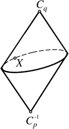
Figure 1: For any two-mode Gaussian state with CM $\gamma=C_{q}\oplus C_{p}$ the Gaussian Entanglement of Formation is given by the entanglement of the least entangled pure state with CM $\gamma_{p}=X\oplus X^{-1}$ which is such that $C_{p}^{-1}\leq X\leq C_{q}$. Moreover, the optimal $X$ can be shown to lie on the rim of the intersection of the forward and backward cones of $C_{p}^{-1}$ and $C_{q}$ respectively.

The covariance matrix in the normal form of Eq. (15) only contains terms which are quadratic in the momenta but has no linear contributions. This implies that the state remains invariant under momentum reversal $P\mapsto-P$ and since this can be interpreted as complex conjugation, the respective density operator is real (in position representation).

Eq. (16) gives the covariance matrix of a pure Gaussian state with respective wave function

$$\Psi(x)=|\pi X|^{-\frac{1}{4}}\exp{\big{[}-\frac{1}{2}x^{T}(X^{-1}-iY)x\big{]}},$$ (20)

which in turn becomes real if $Y=0$. The following Lemma shows that for two-mode states we can, in fact, restrict to these real pure states in the calculation of $E_{G}(\gamma)$:

Lemma 2

Let $\gamma=C_{q}\oplus C_{p}$ be the covariance matrix of a two-mode Gaussian state. Then there exists a pure state with covariance matrix of the same block structure which minimizes $E_{G}$ for $\gamma$.

Proof: We will show that for every $\gamma_{p}(X,Y)\leq\gamma$ of the form in Eq. (16) the covariance matrix $\gamma_{p}(X,0)$ leads to an improvement for $E_{G}$. First note that the block structure of $\gamma$ implies that $\gamma\geq\gamma_{p}(X,\pm Y)$ and thus

$$\gamma \geq \frac{1}{2}\big{[}\gamma_{p}(X,Y)+\gamma_{p}(X,-Y)\big{]}$$ (21)

$$= \gamma_{p}(X,0)+0\oplus(YXY)$$ (22)

$$\geq \gamma_{p}(X,0).$$ (23)

Therefore $\gamma_{p}(X,0)$ is an admissible covariance matrix for the $E_{G}$ optimization problem.

In order to show that $\gamma_{p}(X,0)$ is less entangled than $\gamma_{p}(X,Y)$ we make explicit use of the assumption that we deal with two-mode states. In this case the entanglement is a monotonous function of the determinant of the reduced covariance matrix. The difference of the respective determinants can be calculated straight forward and it is given by

$$\det\big{[}\gamma_{p}^{(A)}(X,Y)\big{]}-\det\big{[}\gamma_{p}^{(A)}(X,0)\big{]}$$ (24)

$$=\ Y_{12}^{2}\ \det\big{[}X\big{]}\ \geq\ 0,$$ (25)

which completes the proof.         

According to Lemma 2 the remaining task for calculating $E_{G}$ is to find the CM $\gamma_{p}=X\oplus X^{-1}$ which has minimal entanglement under the constraint that

$$C_{p}^{-1}\leq X\leq C_{q}.$$ (26)

This inequality has a simple graphical depiction stemming from the fact that the set of positive semi-definite matrices $X$ satisfying an inequality as, e.g. $C_{q}-X\geq 0$, form a cone, which is equivalent to the (backward) light cone of $C_{q}$ in Minkowski space: if we expand a Hermitian $2\times 2$ matrix in terms of Pauli matrices (and the identity), the expansion coefficients play the role of the space-time coordinates and the Minkowski norm is simply given by the determinant of the matrix. Hence, by Eq.(26) $X$ has to lie in the backward cone of $C_{q}$ and in the forward cone of $C_{p}^{-1}$ (see Fig.1).

Instead of minimizing the entropy of the reduced state under this constraint, we may as well minimize the determinant of one of the local covariance matrices

$$m(X) \equiv 1+\frac{X_{12}^{2}}{\det X}=1+\frac{(X^{-1})_{12}^{2}}{\det(X^{-1})}$$ (27)

$$= X_{11}(X^{-1})_{11}\ ,$$ (28)

since, as already stated, this is a monotonously increasing function of the entanglement. Thus we have to find

$$\min_{X}\left\{m(X)\bigm{|}C_{p}^{-1}\leq X\leq C_{q}\right\}$$ (29)

over the real, symmetric 2$\times$2 matrices $X$.

In fact, for the optimal $X$ both inequalities have to be saturated, i. e.

$$\det{(C_{q}-X)}=\det{(X-C_{p}^{-1})}=0.$$ (30)

In order to see this assume we are given a matrix $X$ with $C_{p}^{-1}\leq X<C_{q}$. Then we can decrease the value of $m(X)$ with a matrix $\hat{X}:=X+\epsilon{\bf 1}$ by increasing $\epsilon>0$ until $C_{q}-\hat{X}$ is of rank 1. However, by Eq. (27) the same argument holds for $X^{-1}<C_{p}$.

To depict it geometrically again, the optimal $X$ has to lie on the rim given by the intersection of the backward and forward cones of $C_{q}$ and $C_{p}^{-1}$ respectively. Hence, we have reduced the number of free parameters in the calculation of $E_{G}(\gamma)$ to one angle, which parameterizes the ellipse of this intersection.

For every explicitly given CM $\gamma$ minimizing $m(X)$ on this ellipse is now straight forward. Writing down the resulting value for $E_{G}$ in terms of the general parameters $(n_{a},n_{b},k_{q},k_{p})$ of Eq. (15) leads, however, to quite cumbersome formulae involving the roots of a forth order polynomial. Since not much insight is coming out of these expressions we refrain from writing them down explicitly and continue with discussing the special case $n_{a}=n_{b}$ for which we obtain a simple formula for $E_{G}$.

Nevertheless, for an arbitrary but explicitly given $\gamma$ the remaining variation under the constraint in Eq.(30) is a simple exercise which can be solved analytically with the help of any computer algebra program. For some examples, see Sec. VIII.

VI Symmetric states

Symmetric two-mode Gaussian states with CM of the form in Eq. (15) with $n_{a}=n_{b}\equiv n$ arise naturally when the two beams of a two-mode squeezed state are sent through identical lossy fibers Kimble and Walls (1987) (see also Sec.VIII). The entanglement of formation $E_{F}$ of these states was calculated in Giedke et al. (2003a) and it was proven that a decomposition into Gaussian states gives rise to the optimal value. Together with the obvious fact that $E_{G}$ is an upper bound for $E_{F}$ this implies that $E_{G}=E_{F}$ in this case. Since the calculation of $E_{F}$ is however quite technical and in order to make the present article more self-contained, we provide in the following a simpler way to obtain $E_{G}$.

In principle we could utilize the general results of the previous section, which simplify greatly for the symmetric case. However, we give an alternative proof and reduce the result to the fact that the optimal $\gamma_{p}$ in Eq. (9) has the same logarithmic negativity Vidal and Werner (2002) as $\gamma$. A similar argument is used in Sec. VII to prove additivity of $E_{G}$.

Prop. 2 ($E_{G}$ for symmetric states)

For symmetric $1\times 1$ Gaussian states, i.e. states whose CM $\gamma$ is characterized by local invariants $(n,n,k_{q},k_{p})$, the Gaussian entanglement of formation is given by

$$E_{G}(\gamma)=H(r_{0}),$$ (31)

where the minimum two-mode squeezing required is given by

$$r_{0}=\frac{1}{2}\ln[(n-k_{q})(n+k_{p})]$$ (32)

and $H(r)$ is defined in Eq. (8).

Proof: First, instead of $\gamma$ we consider the locally equivalent CM $\gamma^{\prime}$ which is obtained from $\gamma$ by squeezing both $Q_{A}$ and $Q_{B}$ by $\lambda=[(n+k_{p})/(n-k_{q})]^{1/4}$. Clearly the CM $\gamma^{\prime}$ has the same $E_{G}$ as $\gamma$. It is straightforward to check that the pure two-mode squeezed state with two-mode squeezing parameter $r_{0}$ and corresponding CM $\gamma(r_{0})$ is indeed smaller than $\gamma^{\prime}$.

That there can be no pure state $\gamma_{p}$ with less entanglement satisfying $\gamma_{p}\leq\gamma^{\prime}$ follows from the monotonic dependence of pure state entanglement on the two-mode squeezing parameter: any pure two-mode Gaussian state is locally equivalent to a two-mode squeezed state $\gamma(r)$ and its entanglement is given by $H(r)$. An important entanglement-related characteristic of these CMs are the symplectic eigenvalues of the partially transposed CM Vidal and Werner (2002), in particular those smaller than one. They are invariant under local unitary Gaussian operations and for the two-mode squeezed state given by $e^{\pm r}$. For the symmetric CM $\gamma$ they are $\sqrt{(n\mp k_{q})(n\pm k_{p})}$. Thus the smallest symplectic eigenvalues of $\gamma$ and $\gamma(r_{0})$ coincide.

For positive matrices $A\geq B$ implies $a_{k}\geq b_{k}$, where $a_{k}$ ($b_{k}$) denote the ordered symplectic eigenvalues of $A$ ($B$) Giedke et al. (2003b). Since the ordering $A\geq B$ is preserved under partial transposition, all pure states with less entanglement than $\gamma(r_{0})$ cannot possibly satisfy $\gamma\geq\gamma_{p}$, hence $r_{0}$ is optimal.         

Thus for symmetric states $\gamma$ the optimal pure state $\gamma_{p}$ is characterized by the fact that the smallest symplectic eigenvalues $s_{1}(\tilde{\gamma})$ and $s_{1}(\tilde{\gamma}_{p})$ of the two partially transposed CMs are identical. According to Vidal and Werner (2002) this implies that the logarithmic negativity, $E_{N}(\gamma)=-\frac{1}{2}\ln[s_{1}(\tilde{\gamma})]$ of both states is the same, i.e., in the optimal decomposition pure Gaussian states are mixed such that “no negativity is lost” in the mixing process. For non-symmetric states this is no longer possible and $s_{1}(\tilde{\gamma})$ is strictly larger than $s_{1}(\tilde{\gamma}_{p})$, i.e. more entanglement is needed to form $\gamma$ than required by its negativity.

VII Additivity

One longstanding question about the entanglement of formation is if it is additive, that is whether $E_{F}(\rho_{1}\otimes\rho_{2})=E_{F}(\rho_{1})+E_{F}(\rho_{2})$ or whether one may get an “entanglement discount” when generating several states at a time. Here we show that for symmetric Gaussian states the Gaussian entanglement of formation $E_{G}$ is additive. Since for these states $E_{G}$ was shown Giedke et al. (2003a) to equal $E_{F}$ this may hint at additivity of even the latter quantity for Gaussian states.

Prop. 3 ($E_{G}$ is additive for symmetric states)

Let $\gamma_{l},l=1,\dots,N$ describe symmetric Gaussian states with local invariants $(n_{l},n_{l},k_{q,l},k_{p,l})$ and let $\Gamma=\oplus_{l=1}^{N}\gamma_{l}$ describe the tensor product of these states, then

$$E_{G}(\Gamma)=\sum_{l}E_{G}(\gamma_{l}).$$ (33)

Proof: Let the logarithmic negativity of the $k$th state be $r_{k}$, and assume $r_{k+1}\leq r_{k}$. To show additivity, we use again that $A\geq B>0$ implies $a_{k}\geq b_{k}$ for the ordered symplectic eigenvalues of $A(B)$.

Let $\Gamma_{p}\leq\Gamma$ be a pure $N\times N$-mode CM. Consider the partially transposed CM $\tilde{\Gamma}$. We have

$$\tilde{\Gamma}\geq\tilde{\Gamma}_{p},$$

which implies $s_{k}\geq s_{k}^{\prime}$, where $\{s_{k},k=1,...,N\}$ denote the (descendingly ordered) symplectic eigenvalues of $\tilde{\Gamma}$, and $s_{k}^{\prime}$ the same for $\tilde{\Gamma}_{p}$.

All pure bipartite Gaussian states are locally equivalent to a tensor product of two-mode squeezed states Holevo and Werner (2001) with (ordered) two-mode squeezing parameters $t_{k}$. For the following we only need to look at the $N$ smallest symplectic eigenvalues. For these we have

$$s^{\prime}_{k}=e^{-t_{k}}\,\,\,\mbox{for $\Gamma_{p}$}$$

and

$$s_{k}=e^{-r_{k}}\,\,\,\mbox{for $\Gamma$}.$$

Hence $\Gamma\geq\Gamma_{p}$ implies $t_{k}\geq r_{k}$, i.e., the optimal joint decomposition is the tensor product of the optimal decompositions for the individual copies. Thus $E_{G}$ is additive.         

For the non-symmetric case the optimal individual decomposition does no longer allow $t_{k}=r_{k}$, i.e. more entanglement than required by the logarithmic negativity must be expended to produce $\rho$. Therefore, the previous argument does not hold and the question of additivity of $E_{G}$ remains open for general $1\times 1$ Gaussian states.

VIII Examples

In this section we will apply the Gaussian Entanglement of Formation to a simple practical example. Consider a two-mode squeezed state (TMSS) with CM

$$\begin{gathered}\gamma=\begin{pmatrix}c&0&-s&0\\ 0&c&0&s\\ -s&0&c&0\\ 0&s&0&c\end{pmatrix},\\ c=\cosh{2r},\quad s=\sinh{2r},\end{gathered}$$ (34)

which is to be distributed between two parties by means of a lossy optical fiber. There are two extremal settings for the transmission of the state which may lead to different values for the distributed entanglement: The source could be placed either at one party’s site (“asymmetric setting”) or halfway between both parties (“symmetric setting”). In the former case, one mode is transmitted through the whole length of the fiber while the other one is retained unaffected, in the latter both modes are transmitted through half the length of the fiber each. It turns out that depending on thermal noise and transmission length, one or the other setting yields more entanglement for the distributed state from a given squeezing of the initial state.

According to Duan and Guo (1997) the Gaussian state after transmission through the fiber has a CM

$$\gamma^{\prime}=\begin{pmatrix}c_{1}^{\prime}&0&-s^{\prime}&0\\ 0&c_{1}^{\prime}&0&s^{\prime}\\ -s^{\prime}&0&c_{2}^{\prime}&0\\ 0&s^{\prime}&0&c_{2}^{\prime}\end{pmatrix}$$ (35)

$$\begin{aligned} &\text{ with }c_{i}^{\prime}=c\,T_{i}^{2}+(2N_{\text{th}}+1)\,(1-T_{i}^{2})\text{ for }i=1,2\\ &\text{ and }s^{\prime}=s\,T_{1}\,T_{2}.\end{aligned}$$

Here $T_{1}$, $T_{2}$ are the transmission coefficients of the fiber for the respective modes and the fiber is in a thermal state with mean number of photons $N_{\text{th}}$, which is in turn related to a “temperature” $\tau$ by $N_{\text{th}}=(\exp(1/\tau)-1)^{-1}$. Note that in quantum optical settings using optical frequencies we have $\tau=0$.

Depending on the setting, the transmission coefficients take on the values $T_{1}=e^{-l/l_{\text{A}}},T_{2}=1$ (asymmetric setting) or $T_{1}=T_{2}=e^{-l/(2l_{\text{A}})}$ (symmetric setting) where $l/l_{\text{A}}$ denotes the total length $l$ of the fiber in units of the absorption length $l_{\text{A}}$. As an example, we compare the two settings for a TMSS with $r=1$. While for temperature $\tau=0$ (Fig. 2) the asymmetric setting always yields a higher entanglement for the final state, at finite temperature $\tau=1$ (Fig. 3) the symmetric setting is to be preferred for longer ranges.

Figure 2: Gaussian Entanglement of Formation (in units of ebits) for a TMSS with $r=1$ after transmission through a lossy optical fiber at temperature $\tau=0$. The plot shows $E_{G}(\rho)$ versus transmission length $l/l_{\text{A}}$ for the symmetric and asymmetric setting (dotted and solid line, respectively).

Figure 3: Gaussian Entanglement of Formation (in units of ebits) for a TMSS with $r=1$ after transmission through a lossy optical fiber at temperature $\tau=1$. The plot shows $E_{G}(\rho)$ versus transmission length $l/l_{\text{A}}$ for the symmetric and asymmetric setting (dotted and solid line, respectively).

Figure 4: Gaussian Entanglement of Formation (in units of ebits) for a TMSS with initial squeezing $r$ after symmetric transmission through a lossy optical fiber at zero temperature. $l/l_{\text{A}}$ is the transmission length in units of the absorption length.

Fig. 4 shows $E_{G}$ as a function of the initial squeezing $r$ and the transmission length $l$ for the symmetric setting at zero temperature. As already indicated in Scheel et al. (2000); Scheel and Welsch (2001) increasing the squeezing over a certain threshold has only a negligible effect on the transmitted entanglement already after a small fraction of the absorption length.

IX Conclusion

We introduced a Gaussian version of the Entanglement of Formation by taking into account only decompositions into pure Gaussian states. On Gaussian states this is a proper entanglement measure in the sense that it is non-increasing under GLOCC operations. Moreover, it is an upper bound for the full Entanglement of Formation which is tight and additive at least for symmetric two-mode Gaussian states. However, it remains an open question whether this is true for all Gaussian states.

We have shown how to analytically calculate $E_{G}$ for all two-mode Gaussian states and given a simple formula for the symmetric case. For multimode bipartite states, the (numerical) computation of $E_{G}$ becomes rapidly more difficult: Although Proposition 1 still allows to replace the minimization over all possible decomposition into pure Gaussian states by the minimization over the (for the $n\times n$ case) $2n(2n+1)$ parameter set of pure $2n$-mode covariance matrices the further simplifications used in the $1\times 1$ case are no longer available and the minimization is no longer easy. To compute $E_{G}$ for interesting multi-mode states such as two copies on non-symmetric $1\times 1$ states or bound entangled states Werner and Wolf (2001) new methods need to be developed.

GG and MMW thank Pranaw Rungta for interesting discussion during the ESF QIT conference in Gdansk, 2001. Funding by the European Union project QUPRODIS and the German National Academic Foundation (OK) and financial support by the A2 and A8 consortia is gratefully acknowledged.

Appendix A Proof of Lemma 3

The following Lemma about decompositions of classical multivariate Gaussian distributions is used in the proof of Prop. 1.

Lemma 3

Let

$$G(A,a,x):=|A|^{\frac{1}{2}}(2\pi)^{-\frac{n}{2}}\ e^{-\frac{1}{2}(x-a)^{T}A(x-a)},\quad x,a\in\mathbb{R}^{n}$$ (36)

be a Gaussian probability distribution with symmetric $A>0$ and consider an arbitrary convex decomposition of $G(A,0,x)$ into other Gaussian distributions of this form:

$$G(A,0,x)=\int\mu(dB,db)G(B,b,x).$$ (37)

Then all the distributions contributing to this decomposition have to satisfy $B\geq A$ in the sense that

$$\mu\Big{(}\big{\{}(B,b)\ \big{|}\ \exists_{x}:x^{T}(A-B)x>0\big{\}}\Big{)}=0.$$ (38)

Proof: Let us first define a set

$$S(x,\epsilon) := \Big{\{}(B,b)\ \big{|}\ x^{T}Ax-\epsilon||x||^{2}\geq x^{T}Bx\Big{\}}.$$ (39)

Integrating Eq. (37) only over $S(x,\epsilon)$ leads then to a lower bound on $G(A,0,x)$:

$$G(A,0,x)\geq\int_{S(x,\epsilon)}\mu(dB,db)G(B,b,x).$$ (40)

Inserting $G(A,0,x)$ and $G(B,b,x)$ we can symmetrize inequality (40) with respect to $x\mapsto-x$, which leads to

$$|A|^{\frac{1}{2}}e^{-\frac{1}{2}x^{T}Ax} \geq \int_{S(x,\epsilon)}\mu(dB,db)\ |B|^{\frac{1}{2}}\cosh{(x^{T}Bb)}$$ (41)

$$\quad e^{-\frac{1}{2}(x^{T}Bx+b^{T}Bb)}.$$

Utilizing $\cosh\geq 1$ and the defining property of the set $S(x,\epsilon)$ we have

$$|A|^{\frac{1}{2}}e^{-\frac{\epsilon}{2}||x||^{2}}\geq\int_{S(x,\epsilon)}\mu(dB,db)\ |B|^{\frac{1}{2}}e^{-\frac{1}{2}b^{T}Bb}.$$ (42)

Note that the r.h.s. of Eq. (42) does no longer depend on the norm of $x$ but merely on its angular components. Taking the limit $||x||\rightarrow\infty$ implies then that $S(x,\epsilon)$ is of measure zero for every $\epsilon>0$. Moreover, every countable union of such sets is of measure zero. In particular:

$$\bigcup_{x\in\mathbb{Q}^{n}}\bigcup_{m\in\mathbb{N}}S(x,\frac{1}{m})\ =$$ (44)

$$= \Big{\{}(B,b)\big{|}\exists x\in\mathbb{Q}^{n},\exists m\in\mathbb{N}:$$

$$\qquad x^{T}Ax\geq x^{T}Bx+\frac{1}{m}||x||^{2}\Big{\}}$$

$$= \Big{\{}(B,b)\big{|}\exists x\in\mathbb{Q}^{n}:x^{T}Ax>x^{T}Bx\Big{\}}$$ (45)

$$= \Big{\{}(B,b)\big{|}\exists x\in\mathbb{R}^{n}:x^{T}(A-B)x>0\Big{\}},$$ (46)

where we have of course used that $\mathbb{Q}^{n}$ is dense in $\mathbb{R}^{n}$.

References

- Donald et al. (2002) M. J. Donald, M. Horodecki, and O. Rudolph, J. Math. Phys. 43, 4252 (2002), eprint quant-ph/0105017.
- Vidal (2000) G. Vidal, J. Mod. Opt. 47, 355 (2000), eprint quant-ph/9807077.
- Popescu and Rohrlich (1997) S. Popescu and D. Rohrlich, Phys. Rev. A 56, R3319 (1997).
- Horodecki (2001) M. Horodecki, J. Quant. Inf. Comp. 1, 3 (2001).
- Bennett et al. (1996) C. H. Bennett, D. P. DiVincenzo, J. A. Smolin, and W. K. Wootters, Phys. Rev. A 54, 3824 (1996), eprint quant-ph/9604024.
- Wootters (1998) W. K. Wootters, Phys. Rev. Lett. 80, 2245 (1998), eprint quant-ph/9709029.
- Terhal and Vollbrecht (2000) B. M. Terhal and K. G. H. Vollbrecht (2000), eprint quant-ph/0005062.
- Vollbrecht and Werner (2000) K. G. H. Vollbrecht and R. F. Werner, Phys. Rev. A 64, 062307 (2000), eprint quant-ph/0001095.
- Giedke et al. (2003a) G. Giedke, M. M. Wolf, O. Krüger, R. F. Werner, and J. I. Cirac, to appear in Phys. Rev. Lett., (2003a), eprint quant-ph/0304042.
- Vogel et al. (2001) W. Vogel, D.-G. Welsch, and S. Wallentowitz, Quantum Optics. An Introduction (Wiley-VCH, 2001).
- Julsgaard et al. (2000) B. Julsgaard, A. Kozhekin, and E. S. Polzik, Nature 413, 400 (2000).
- Braunstein and Pati (2003) S. L. Braunstein and A. K. Pati, eds., Quantum Information with Continuous Variables (Kluwer Academic, Dordrecht, 2003).
- Holevo and Werner (2001) A. Holevo and R. F. Werner, Phys. Rev. A 63, 032312 (2001), eprint quant-ph/9912067.
- Grossmann (1976) A. Grossmann, Commun. Math. Phys. 48, 191 (1976).
- Giedke and Cirac (2002) G. Giedke and J. I. Cirac, Phys. Rev. A 66, 032316 (2002), eprint quant-ph/0204085.
- Fiurášek (2002) J. Fiurášek, Phys. Rev. Lett. 89, 137904 (2002), eprint quant-ph/0204069.
- Horn and Johnson (1987) R. A. Horn and C. R. Johnson, Matrix Analysis (Cambridge University Press, 1987).
- Giedke et al. (2003b) G. Giedke, J. Eisert, J. I. Cirac, and M. B. Plenio, J. Quant. Inf. Comp. 3(3), 211 (2003b), eprint quant-ph/0301038.
- Duan et al. (2000) L.-M. Duan, G. Giedke, J. I. Cirac, and P. Zoller, Phys. Rev. Lett. 84, 2722 (2000), eprint quant-ph/9908056.
- Simon (2000) R. Simon, Phys. Rev. Lett. 84, 2726 (2000), eprint quant-ph/9909044.
- Kimble and Walls (1987) H. J. Kimble and D. F. Walls, J. Opt. Soc. Am. B 4, 10 (1987).
- Vidal and Werner (2002) G. Vidal and R. F. Werner, Phys. Rev. A 65, 032314 (2002), eprint quant-ph/0102117.
- Duan and Guo (1997) L.-M. Duan and G. Guo, J. Quant. Semiclass. Opt. 9, 953 (1997).
- Scheel et al. (2000) S. Scheel, T. Opatrny, and D.-G. Welsch, (2000), eprint quant-ph/0006026.
- Scheel and Welsch (2001) S. Scheel and D.-G. Welsch, Phys. Rev. A 64, 063811, (2001), eprint quant-ph/0103167.
- Werner and Wolf (2001) R. F. Werner and M. M. Wolf, Phys. Rev. Lett. 86, 3658 (2001), eprint quant-ph/0009118.