Quantum Correlation Games

Abstract

A new approach to play games quantum mechanically is proposed. We consider two players who perform measurements in an EPR-type setting. The payoff relations are defined as functions of correlations, i.e. without reference to classical or quantum mechanics. Classical bi-matrix games are reproduced if the input states are classical and perfectly anti-correlated, that is, for a classical correlation game. However, for a quantum correlation game, with an entangled singlet state as input, qualitatively different solutions are obtained. For example, the Prisoners’ Dilemma acquires a Nash equilibrium if the players both apply a mixed strategy. It appears to be conceptually impossible to reproduce the properties of quantum correlation games within the framework of classical games.

PACS: 03.67.-a, 02.50.Le

1 Introduction

To process information has been conceived for a long time as a purely mathematical task, independent of the carrier of information. However, problems such as identifying a marked object in a database [1] or the factorization of large integer numbers [2] are solved in a highly efficient way if information is stored and processed quantum mechanically. Hence, the theory of quantum information came into existence generalizing classical bits to qubits: linear combinations of classically incompatible states are possible, and they can be processed simultaneously.

Game theory [3], a tool to take decisions in a rational way, has been proposed as another promising candidate to benefit from a quantum mechanical implementation [4]. Based on their knowledge of the circumstances, players in a classical game select from a set of possible moves or actions to maximize their payoffs. In its quantum version, unexpected moves may provide new solutions to the game; a strategy which includes quantum moves may outperform a classical strategy [5]. Opinions about the true quantum character of such games are divided, however. It has been argued that quantized games are nothing but disguised classical games [6]. In other words, to quantize a game is claimed equivalent to replacing the original game by a different classical game.

In the present paper, we associate a quantum game with a classical game in a way which addresses this criticism by imposing two constraints:

1. The players choose their moves (or actions) from the same set in both the classical and the quantized game.

2. The players agree on explicit expressions for their payoffs which must not be modified when switching between the classical and the quantized version of the game.

Games with these properties are expected to be immune against the criticism raised above. In the new setting, the only ‘parameter’ is the input state on which the players act, and its nature will determine the classical or quantum character of the game. Our approach to quantum games, tailored to satisfy both (c1) and (c2), is inspired by Bell’s work [7]: correlations of measurement outcomes are essential. Effectively, we will define payoff relations in terms of correlations - these payoffs will become sensitive to the classical or quantum nature of the input allowing for modified Nash equilibria.

Section $2$ introduces our notation of classical games. Then, games will be set up in a way which resembles an EPR experiment. In Section $4$, correlation games will be defined through payoffs depending explicitly on correlations. If played on a classical input state, they reproduce classical bi-matrix games. New advantageous strategies may emerge, however, if the same payoff relations are used in the quantum mechanical setting, as shown in Section $5$. Finally, we discuss achievements and limitations of our approach.

2 Matrix games and payoffs

Consider a matrix game [8] for two players, called Alice and Bob. A large set of identical objects are prepared in definite states, not necessarily known to the players. Each object splits into two equivalent ‘halves’ handed over to Alice and Bob simultaneously. Let the players agree beforehand on the following rules:

1. Alice and Bob may either play the identity move $I$ or perform actions $S_{A}$ and $S_{B}$, respectively. The moves $S_{A,B}$ (and $I$) consist of unique actions such as flipping a coin (or not) and possibly reading it.

2. The players agree upon payoff relations $P_{A,B}(p_{A},p_{B})$ which determine their awards as functions of their strategies, that is, the moves with probabilities $p_{A,B}$ assigned to them.

3. The players fix their strategies for repeated runs of the game. In a mixed strategy Alice plays the identity move $I$ with probability $p_{A}$, say, while she plays $S_{A}$ with probability ${\overline{p}}_{A}=1-p_{A}$, and similarly for Bob. In a pure strategy, each player performs the same action in each run.

4. Whenever the players receive their part of the system, they perform a move consistent with their strategy.

5. The players inform an arbiter about their actions taken in each individual run. After a large number of runs, they are rewarded according to the agreed payoff relations $P_{A,B}$. The existence of the arbiter is for clarity only: alternatively, the players get together to decide on their payoffs.

These conventions are sufficient to play a classical game. As an example, consider the class of symmetric bi-matrix games with payoff relations

$$P_{A}(p_{A},p_{B}) = Kp_{A}p_{B}+Lp_{A}+Mp_{B}+N,$$

$$P_{B}(p_{A},p_{B}) = Kp_{A}p_{B}+Mp_{A}+Lp_{B}+N,$$ (1)

where $K,L,M,$ and $N$ are real numbers. Being functions of two real variables, $0\leq p_{A,B}\leq 1$, the payoff relations $P_{A,B}$ reflect that each player may chose a strategy from a continuous one-parameter set. The game is symmetric since

$$P_{A}(p_{A},p_{B})=P_{B}(p_{B},p_{A}).$$ (2)

Look at pure strategies with $p_{A,B}=0$ or $1$ in Eq. (1):

$$P_{A}(1,1)=P_{B}(1,1) = r=K+L+M+N,$$

$$P_{A}(1,0)=P_{B}(0,1) = s=L+N,$$

$$P_{A}(0,1)=P_{B}(1,0) = t=M+N,$$

$$P_{A}(0,0)=P_{B}(0,0) = u=N,$$ (3)

leading to the payoff matrix for this game

$$\begin{array}[]{c}\text{Alice}\end{array}\begin{array}[]{c}I\\ S_{A}\end{array}\overset{\overset{\begin{array}[]{c}\text{Bob}\end{array}}{\begin{array}[]{cc}I&S_{B}\end{array}}}{\left(\begin{array}[]{cc}(r,r)&(s,t)\\ (t,s)&(u,u)\end{array}\right).}$$ (4)

In words: If both Alice and Bob play the identity $I$, they are paid $r$ units; Alice playing the identity $I$ and Bob playing $S_{B}$ pays $s$ and $t$ units to them, respectively; etc. Knowledge of the payoff matrix (4) and the probabilities $p_{A,B}$ is, in fact, equivalent to (1) since the expected payoffs $P_{A,B}$ are obtained by averaging (4) over many runs.

Let Alice and Bob act rationally: they will try to maximize their payoffs by an appropriate strategy [3]. If the entries of the matrix (4) satisfy $s<u<r<t$, the Prisoners’ Dilemma [8] arises: the players opt for strategies in which unilateral deviations are disadvantageous; nevertheless, the resulting solution of the game, a Nash equilibrium, does not maximize their payoffs.

In view of the conditions (c1) and (c2) the form of the payoff relations $P_{A,B}$ in (1) seems to leave no room to introduce quantum games which would differ from classical ones. In the following, we will introduce payoff relations which are sensitive to whether a game is played on classical or quantum objects. With classical input, they will reproduce the classical game, and the conditions (c1) and (c2) will be respected throughout.

3 EPR-type setting of matrix games

Correlation games will be defined in a setting which is inspired by EPR-type experiments [9]. Alice and Bob are spatially separated, and they share information about a Cartesian coordinate system with axes $\mathbf{e}_{x},\mathbf{e}_{y},\mathbf{e}_{z}$. The physical input used in a correlation game is a large number of identical systems with zero angular momentum, $\mathbf{J}=0$. Each system decomposes into a pair of objects which carry perfectly anti-correlated angular momenta $\mathbf{J}_{A,B}$, i.e. $\mathbf{J}_{A}+\mathbf{J}_{B}=0$.

In each run, Alice and Bob will measure the dichotomic variable $\mathbf{e}\cdot\mathbf{J}/|\mathbf{e}\cdot\mathbf{J}|$ of their halves along the common $z$-axis ($\mathbf{e}\rightarrow\mathbf{e}_{z}$) or along specific directions $\mathbf{e}\rightarrow\mathbf{e}_{A}$ and $\mathbf{e}\rightarrow\mathbf{e}_{B}$ in two planes $\mathcal{P}_{A}$ and $\mathcal{P}_{B}$, respectively, each containing the $z$-axis, as shown in Fig. $1$. The vectors $\mathbf{e}_{A}$ and $\mathbf{e}_{B}$ are characterized by the angles $\theta_{A}$ and $\theta_{B}$ which they enclose with the $z$-axis:

$$\mathbf{e}_{z}\cdot\mathbf{e}_{A,B}=\cos\theta_{A,B}\text{ },\qquad 0\leq\theta_{A,B}\leq\pi.$$ (5)

In principle, Alice and Bob could be given the choice of both the directions $\mathbf{e}_{A,B}$ and the probabilities $p_{A,B}$. However, in traditional matrix games each player has access to one continuous variable only, namely $p_{A,B}$. To remain within this framework, we impose a relation between the probabilities $p_{A,B}\in[0,1]$, and the angles $\theta_{A,B}\in[0,\pi]$:

$$p_{A,B}=g(\theta_{A,B})\,.$$ (6)

The function $g$ maps the interval $[0,\pi]$ to $[0,1]$, and it is specified before the game begins. This function is, in general, not required to be invertible or continuous. Relation (6) says that Alice must play the identity with probability $p_{A}\equiv g(\theta_{A})$ if she decides to select the direction $\mathbf{e}_{A}$ as her alternative to $\mathbf{e}_{z}$; furthermore, she measures with probability $\overline{p}_{A}=1-g(\theta_{A})$ along $\mathbf{e}_{A}$. For an invertible function $g$, Alice can choose either a probability $p_{A}$ or a direction $\theta_{A}$ and find the other variable from Eq. (6). If the function $g$ is not invertible, some values of probability are associated with more than one angle, and it is more natural to have the players choose a direction first. For simplicity we will assume the function $g$ to be invertible, if not specified otherwise.

According to her chosen strategy, Alice will measure the quantity $\mathbf{e}\cdot\mathbf{J}/|\mathbf{e}\cdot\mathbf{J}|$ with probability $p_{A}$ along the $z$-axis, and with probability $\overline{p}_{A}=1-p_{A}$ along the direction $\mathbf{e}_{A}$. Similarly, Bob can play a mixed strategy, measuring along the directions $\mathbf{e}_{z}$ or $\mathbf{e}_{B}$ with probabilities $p_{B}$ and $\overline{p}_{B}$, respectively. Hence, Alice’s moves consists of either $S_{A}$ (rotating a Stern-Gerlach type apparatus from $\mathbf{e}_{z}$ to $\mathbf{e}_{A}$, followed by a measurement) or of $I$ (a measurement along $\mathbf{e}_{z}$ with no previous rotation). Bob’s moves $I$ and $S_{B}$ are defined similarly. It is convenient to denote the outcomes of measurements along the directions $\mathbf{e}_{A},\mathbf{e}_{B}$, and $\mathbf{e}_{z},$ by $a,b,$ and $c$, respectively.

Figure 1: The players’ strategies consist of defining angles $\theta_{A,B}$ which the directions $\mathbf{e}_{A,B}$ make with the $z$-axis; for simplicity, the planes $\mathcal{P}_{A,B}$ are chosen as the $xz$- and $yz$-plane, respectively.

After each run, the players inform the arbiter about the chosen directions and the result of their measurements. After $N\rightarrow\infty$ runs of the game, the arbiter possesses a list $\mathcal{L}$ indicating the directions of the measurements selected by the players and the measured values of the quantity $\mathbf{e}\cdot\mathbf{J}/|\mathbf{e}\cdot\mathbf{J}|$. The arbiter uses the list to determine the strategies played by Alice and Bob by simply counting the number of times ($N_{A}$, say) that Alice measured along $\mathbf{e}_{A}$, giving $p_{A}=\underset{N\rightarrow\infty}{\lim}(N-N_{A})/N$, etc. Finally, the players are rewarded according to the payoff relations (1).

4 Correlation games

We now develop a new perspective of matrix games in the EPR-type setting. The basic idea is to define payoffs $P_{A,B}=P_{A,B}(\left\langle ac\right\rangle,\left\langle cb\right\rangle)$ which depend explicitly on the correlations of the actual measurements performed by Alice and Bob. The arbiter will extract the numerical values of the correlations $\left\langle ac\right\rangle$ etc. from the list $\mathcal{L}$ in the usual way. Consider, for example, all cases with Alice measuring along $\mathbf{e}_{A}$ and Bob along $\mathbf{e}_{z}$. If there are $N_{ac}$ such runs, the correlation of the measurements is defined by

$$\left\langle ac\right\rangle=\lim_{N_{ac}\rightarrow\infty}\left(\sum_{n=1}^{N_{ac}}\frac{a_{n}c_{n}}{N_{ac}}\right)\,,$$ (7)

where $a_{n}$ and $c_{n}$ take the values $\pm 1$ [9]. The correlations $\left\langle ab\right\rangle$ and $\left\langle cb\right\rangle$ are defined similarly.

A symmetric bi-matrix correlation game is determined by a function $g$ in (6) and by the relations

$$P_{A}(\left\langle ac\right\rangle,\left\langle cb\right\rangle) = K\text{ }G(\left\langle ac\right\rangle)G(\left\langle cb\right\rangle)+L\text{ }G(\left\langle ac\right\rangle)+M\text{ }G(\left\langle cb\right\rangle)+N,$$

$$P_{B}(\left\langle ac\right\rangle,\left\langle cb\right\rangle) = K\text{ }G(\left\langle ac\right\rangle)G(\left\langle cb\right\rangle)+M\text{ }G(\left\langle ac\right\rangle)+L\text{ }G(\left\langle cb\right\rangle)+N,$$ (8)

where, in view of later developments, the function $G$ is taken to be

$$G(x)=g\left(\frac{\pi}{2}(1+x)\right)\,,\quad x\in[0,1].$$ (9)

As they stand, the payoff relations (8) do refer to neither a classical nor a quantum mechanical input. Hence, condition (c2) from above is satisfied: the payoff relations used in the classical and the quantum version of the game are identical, namely given by Eqs. (8). Furthermore, Alice and Bob choose from the same set of moves in both versions of the game: they select directions $\mathbf{e}_{A}$ and $\mathbf{e}_{B}$ (with probabilities $p_{A,B}$ associated with $\theta_{A,B}$ via (6)) so that condition (c1) is satisfied. Nevertheless, the solutions of the correlation game (8) will depend on the input being either a classical or a quantum mechanical anti-correlated state.

4.1 Classical correlation games

Alice and Bob play a classical correlation game if they receive classically anti-correlated pairs and use the payoff relations (8). In this case, the payoffs turn into

$$P_{A,B}^{cl}=P_{A,B}(\left\langle ac\right\rangle_{cl},\left\langle cb\right\rangle_{cl}),$$ (10)

where the correlations, characteristic for classically anti-correlated systems [9], are given by

$$\left\langle ac\right\rangle_{cl} = -1+2\theta_{A}/\pi,$$

$$\left\langle cb\right\rangle_{cl} = -1+2\theta_{B}/\pi.$$ (11)

Use now the definition of the function $G$ in (9) and the link (6) between probabilities $p_{A,B}$ and angles $\theta_{A,B}$ to obtain

$$G(\langle ac\rangle) = g(\theta_{A})=p_{A},$$ (12)

$$G(\langle cb\rangle) = g(\theta_{B})=p_{B}.$$ (13)

Hence, for classical input Eqs. (8) reproduce the payoffs of a symmetric bi-matrix game (1),

$$P_{A}^{cl}(p_{A},p_{B}) = Kp_{A}p_{B}+Lp_{A}+Mp_{B}+N,$$

$$P_{B}^{cl}(p_{A},p_{B}) = Kp_{A}p_{B}+Mp_{A}+Lp_{B}+N.$$ (14)

The game-theoretic analysis of the classical correlation game is now straightforward—for example, appropriate values of the parameters $(r,s,t,u)$ lead to the Prisoners’ Dilemma, for any invertible function $g$.

4.2 Quantum correlation games

Imagine now that Alice and Bob receive quantum mechanical anti-correlated singlet states

$$|\psi\rangle=\frac{1}{\sqrt{2}}\left(|+,-\rangle-|-,+\rangle\right).$$ (15)

They are said to play a quantum correlation game if again they use the payoff relations (8) which read in this case

$$P_{A,B}^{q}=P_{A,B}(\left\langle ac\right\rangle_{q},\left\langle cb\right\rangle_{q}).$$ (16)

As before, Alice and Bob transmit the results of their measurements (on their quantum halves) to the arbiter who, after a large number of runs, determines the correlations $\left\langle ac\right\rangle_{q}$ and $\left\langle cb\right\rangle_{q}$ by the formula (7)

$$\left\langle ac\right\rangle_{q} = -\cos\theta_{A},$$

$$\left\langle cb\right\rangle_{q} = -\cos\theta_{B},$$ (17)

in contrast to (11).

The inverse of relation (6), then, links the probabilities and correlations through

$$\left\langle ac\right\rangle_{q} = -\cos\left(g^{-1}(p_{A})\right),$$

$$\left\langle cb\right\rangle_{q} = -\cos\left(g^{-1}(p_{B})\right).$$ (18)

Plugging these expressions into the right-hand-side of (16), we obtain quantum payoffs:

$$P_{A}^{q}(p_{A},p_{B}) = KQ_{g}(p_{A})Q_{g}(p_{B})+LQ_{g}(p_{A})+MQ_{g}(p_{B})+N,$$

$$P_{B}^{q}(p_{A},p_{B}) = KQ_{g}(p_{A})Q_{g}(p_{B})+MQ_{g}(p_{B})+LQ_{g}(p_{A})+N.$$ (19)

where

$$Q_{g}(p_{A,B})=g\left(\frac{\pi}{2}\left(1-\cos\left(g^{-1}(p_{A,B})\right)\right)\right)\in[0,1].$$ (20)

The payoffs $P_{A,B}^{q}$ turn out to be non-linear functions of the probabilities $p_{A,B}$ while the payoffs $P_{A,B}^{cl}$ of the classical correlation game are bi-linear. This modification has an impact on the solutions of the game as shown in the following section.

5 Nash equilibria of quantum correlation games

What are the properties of the quantum payoffs $P_{A,B}^{q}$ compared to the classical ones, $P_{A,B}^{cl}$? The standard approach to ‘solving games’ consists in studying Nash equilibria. For a bi-matrix game a pair of strategies $(p_{A}^{\star},p_{B}^{\star})$ is a Nash equilibrium if each players’ payoff does not increase upon unilateral deviation from it,

$$P_{A}(p_{A},p_{B}^{\star}) \leq P_{A}(p_{A}^{\star},p_{B}^{\star})\,,\quad\text{for all }p_{A},$$

$$P_{B}(p_{A}^{\star},p_{B}) \leq P_{B}(p_{A}^{\star},p_{B}^{\star})\,,\quad\text{for all }p_{B}.$$ (21)

In the following, we will study the differences between classical and quantum correlation games which are associated with two paradigmatic games: the Prisoners’ Dilemma (PD) and the Battle of Sexes (BoS).

The payoff matrix of the PD has been introduced in (4). It will be convenient to use the notation of game theory: $C\thicksim I$ corresponds to Cooperation, while $D\thicksim S_{A,B}$ is the strategy of Defection. A characteristic feature of this game is that the condition $s<u<r<t$ guarantees that the strategy $D$ dominates the strategy $C$ for both players and that the unique equilibrium at $(D,D)$ is not Pareto optimal. An outcome of a game is Pareto optimal if there is no other outcome that makes one or more players better off and no player worse off. This can be seen in the following way. The conditions (21) read explicitly

$$0 \leq \left(Kp_{B}^{\star}+L\right)(p_{A}^{\star}-p_{A})\text{ },\quad\text{for all }p_{A},$$

$$0 \leq \left(Kp_{A}^{\star}+L\right)(p_{B}^{\star}-p_{B})\text{ },\quad\text{for all }p_{B}.$$ (22)

with $K$ and $L$ from (3). The inequalities have only one solution

$$p_{A}^{\star}=p_{B}^{\star}=0\text{ },$$ (23)

which corresponds to $(D,D)$, a pure strategy for both players. The PD is said to have a pure Nash equilibrium.

The BoS is defined by the following payoff matrix:

$$\begin{array}[]{c}\text{Alice}\end{array}\begin{array}[]{c}I\\ S_{A}\end{array}\overset{\overset{\begin{array}[]{c}\text{Bob}\end{array}}{\begin{array}[]{cc}I&S_{B}\end{array}}}{\left(\begin{array}[]{cc}(\alpha,\beta)&(\gamma,\gamma)\\ (\gamma,\gamma)&(\beta,\alpha)\end{array}\right),}$$ (24)

where $I$ and $S_{A,B}$ are pure strategies and $\alpha>\beta>\gamma$. Three Nash equilibria arise in the classical BoS, two of which are pure: $(I,I)$ and $(S_{A},S_{B})$. The third one is a mixed equilibrium where Alice and Bob play $I$ with probabilities

$$p_{A}^{\star}=\frac{\alpha-\gamma}{\alpha+\beta-2\gamma}\text{ },\qquad p_{B}^{\star}=\frac{\beta-\gamma}{\alpha+\beta-2\gamma}\text{ }.$$ (25)

For the quantum correlation game associated with the generalized PD, the conditions (21) turn into

$$0 \leq \left(KQ_{g}(p_{B}^{\star})+L\right)\left(Q_{g}(p_{A}^{\star})-Q_{g}(p_{A})\right)\,,$$ (26)

$$0 \leq \left(KQ_{g}(p_{A}^{\star})+L\right)\left(Q_{g}(p_{B}^{\star})-Q_{g}(p_{B})\right)\,,$$ (27)

where the range of $Q_{g}(p_{A,B})$ has been defined in (20). Thus, the conditions for a Nash equilibrium of a quantum correlation game are structurally similar to those of the classical game except for non-linear dependence on the probabilities $p_{A,B}$. The only solutions of (27) therefore read

$$Q_{g}({p_{A}^{\star}})=Q_{g}({p_{B}^{\star}})=0\,,$$ (28)

generating upon inversion a Nash equilibrium at

$$(p_{A}^{\star})_{q}=(p_{B}^{\star})_{q}=Q_{g}^{-1}(0)=g\left(\arccos\left(1-\frac{2}{\pi}g^{-1}(0)\right)\right),$$ (29)

where the transformed probabilities now come with a subscript $q$ indicating the presence of quantum correlations. The location of this new equilibrium depends on the actual choice of the function $g$, as is shown below.

Similar arguments apply to the pure Nash equilibria of the BoS game while the mixed classical equilibrium (25) is transformed into

$$(p_{A}^{\star})_{q} = Q_{g}^{-1}(p_{A}^{\star})=g\left(\arccos\left(1-\frac{2}{\pi}g^{-1}(\frac{\alpha-\gamma}{\alpha+\beta-2\gamma})\right)\right),$$

$$(p_{B}^{\star})_{q} = Q_{g}^{-1}(p_{B}^{\star})=g\left(\arccos\left(1-\frac{2}{\pi}g^{-1}(\frac{\beta-\gamma}{\alpha+\beta-2\gamma})\right)\right).$$ (30)

When defining a quantum correlation game we need to specify a function $g$ which establishes the link between probabilities $p_{A,B}$ and angles $\theta_{A,B}$. We will study the properties of quantum correlation games for $g$-functions of increasing complexity. In the simplest case, the function $g$ is ($i$) continuous and invertible; next, we chose a function $g$ being ($ii$) invertible and discontinuous or ($iii$) non-invertible and discontinuous. For simplicity, all examples are worked out for piecewise linear $g$-functions. The generalization to smooth $g$-functions turns out to be straightforward, and the results do not change qualitatively as long as the $g$ function preserves its characteristic features.

($i$) Continuous and invertible g-functions

Consider the function $g_{1}(\theta)=\theta/\pi$ defined for $\theta\in[0,\pi]$. We have $g_{1}(0,\pi)=0$ or $1$, and the classical and quantum correlations coincide at $\theta=0,\pi/2,$ and $\pi$. In view of (29) the function $g_{1}$ can have no effect on pure Nash equilibria and the classical solution of PD is not modified in the quantum game. Fig. 2 shows the function $g_{1}$.

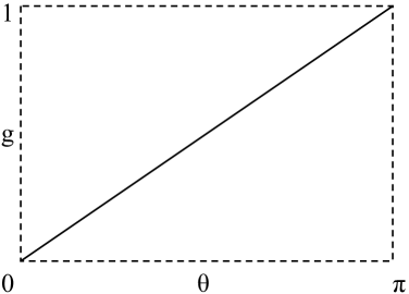
Figure 2: The invertible and continuous $g$-function $g_{1}(\theta)=\theta/\pi$.

However, solutions $p_{A,B}^{\star}\in(0,1)$ correspond to a mixed classical equilibrium. It will be modified if $g(\pi/2)\neq p_{A,B}^{\star}$ i.e. when the angle associated with $p_{A,B}^{\star}$ is different from $\pi/2$. For example with the function $g_{1}(\theta)$ the probabilities of the mixed equilibrium of the quantum correlation BoS are $(p_{A}^{\star})_{q}=1-(1/\pi)\arccos\left\{(\alpha-\gamma)/(\alpha+\beta-2\gamma)\right\}$ and $(p_{B}^{\star})_{q}=1-(1/\pi)\arccos\left\{(\beta-\gamma)/(\alpha+\beta-2\gamma)\right\}$. A similar result holds for the function $g_{2}(\theta)=1-\theta/\pi$.

($ii$) Invertible and discontinuous g-functions

For simplicity we consider invertible functions that are discontinuous at one point only. Piecewise linear functions are typical examples. One such function, shown in Fig. 3, is

$$g_{3}(\theta)=\left\{\begin{array}[]{rcl}\delta(1-\theta/\epsilon)&\text{if}&\theta\in[0,\epsilon]\text{ },\\ \delta+(1-\delta)(\theta-\epsilon)/(\pi-\epsilon)&\text{if}&\theta\in(\epsilon,\pi)\text{ }.\end{array}\right.$$ (31)

The classical solution of PD $p_{A}^{\star}=p_{B}^{\star}=0$ disappears; the new quantum solution is found at

$$(p_{A}^{\star})_{q}=(p_{B}^{\star})_{q}=\left\{\begin{array}[]{rcl}\delta+\frac{(1-\delta)}{(\pi-\epsilon)}\left\{\arccos(1-2\epsilon/\pi)-\epsilon\right\}&\text{if}&\epsilon\in[0,\frac{\pi}{2}]\text{ },\\ \delta\left\{1-\frac{1}{\epsilon}\arccos(1-2\epsilon/\pi)\right\}&\text{if}&\epsilon\in(\frac{\pi}{2},\pi]\text{ }.\end{array}\right.$$ (32)

If, for example, $\delta=1/2$ and $\epsilon=\pi/4,$ we obtain a mixed equilibrium at $(p_{A}^{\star})_{q}=(p_{B}^{\star})_{q}=5/9.$ The appearance of a mixed equilibrium in a quantum correlation PD game is an entirely non-classical feature.

Figure 3: Invertible and discontinuous $g$-function defined in Eq. (31).

The presence of a mixed equilibrium in the quantum correlation PD gives rise to an interesting question: is there a Pareto-optimal solution of $(C,C)$ in a quantum correlation PD with some invertible and discontinuous $g$-function? No such solution exists for invertible and continuous $g$-functions. Also, the $(C,C)$ equilibrium in PD cannot appear in a quantum correlation game played with the function (31): one has $g^{-1}(1)=\pi$ which can not be equal to $g^{-1}(0)$ when $g$ is invertible. As a matter of fact, the solution $(C,C)$ for PD can be realized in a quantum correlation PD if one considers $g$ from (32) with $\epsilon=\pi/2$:

$$g_{4}(\theta)=\left\{\begin{array}[]{rcl}\delta(1-2\theta/\pi)&\text{if}&\theta\in[0,\frac{\pi}{2}]\text{ },\\ 1-2(1-\delta)(\theta-\pi/2)/\pi&\text{if}&\theta\in(\frac{\pi}{2},\pi]\text{ },\end{array}\right.$$ (33)

where $\delta\in(0,1)$, depicted in Fig. 4.

Figure 4: Invertible and discontinuous $g$-function defined in Eq. (33).

This function satisfies $g^{-1}(0)=g^{-1}(1)=\pi/2$. Therefore, one has $\cos\left\{g^{-1}(1)\right\}=1-2g^{-1}(0)/\pi$, which is the condition for $(C,C)$ to be an equilibrium in PD. Cooperation $(C,C)$ will also be an equilibrium in PD if the $g$-function is defined as

$$g_{5}(\theta)=\left\{\begin{array}[]{rcl}2(1-\delta)\theta/\pi+\delta&\text{if}&\theta\in[0,\frac{\pi}{2}]\text{ },\\ 2\delta(\theta-\pi/2)/\pi&\text{if}&\theta\in(\frac{\pi}{2},\pi]\text{ },\end{array}\right.$$ (34)

where $\delta\in(0,1)$. Fig. 5 shows this function.

Figure 5: Invertible and discontinuous $g$-function defined in Eq. (34).

In both cases (33,34), the $g$-function has a discontinuity at $\theta=\pi/2$. With these functions both the pure and mixed classical equilibria of BoS will also be susceptible to change. The shifts in the pure equilibria in BoS will be similar to those of PD but the mixed equilibrium of BoS will move depending on the location of $\delta$.

Another example of an invertible and discontinuous function is given by

$$g_{6}(\theta)=\left\{\begin{array}[]{rcl}(1-\delta)\theta/\epsilon+\delta&\text{if}&\theta\in[0,\epsilon]\text{ },\\ \delta(\pi-\theta)/(\pi-\epsilon)&\text{if}&\theta\in(\epsilon,\pi]\text{ },\end{array}\right.$$ (35)

where $\delta\in(0,1)$ and $\epsilon\in(0,\pi)$ and it is drawn in Fig. 6.

Figure 6: Invertible and discontinuous $g$-function defined in Eq. (35).

With this function the pure classical equilibria $p_{A}^{\star}=p_{B}^{\star}=0$ of PD as well as of BoS remain unaffected because these equilibria require $\theta=\pi,$ and the function is not discontinuous at $\pi$. One notices that if the angle corresponding to a classical equilibrium is $0,\pi/2,$ or $\pi$, and there is no discontinuity at $\pi/2$, then the quantum correlation game can not change that equilibrium. With the function (35) in both PD or BoS the pure equilibrium with $p_{A}^{\star}=p_{B}^{\star}=1$ corresponds to the angle $\theta=\epsilon$ where classical and quantum correlations are different (for $\epsilon\neq\pi/2$). Consequently, the equilibrium $p_{A}^{\star}=p_{B}^{\star}=1$ will be shifted and the new equilibrium depends on the angle $\arccos(1-2\epsilon/\pi)$. The mixed equilibrium of BoS will also be shifted by the function (35). Therefore, one of the pure equilibria and the mixed equilibrium may shift if the $g$-function (35) is chosen. The following function

$$g_{7}(\theta)=\left\{\begin{array}[]{rcl}1-(1-\delta)\theta/\epsilon&\text{if}&\theta\in[0,\epsilon]\,,\\ \delta(\theta-\epsilon)/(\pi-\epsilon)&\text{if}&\theta\in(\epsilon,\pi]\,,\end{array}\right.$$ (36)

where $\delta\in(0,1)$ and $\epsilon\in(0,\pi),$ cannot change the pure equilibrium at $p_{A}^{\star}=p_{B}^{\star}=1$. However, it can affect the equilibrium $p_{A}^{\star}=p_{B}^{\star}=1$, both in PD and BoS, and it can shift the mixed equilibrium of BoS. Fig. 7 shows this function.

Figure 7: Invertible and discontinuous $g$-function defined in Eq. (36).

($iii$) Non-invertible and discontinuous g-functions

A simple case of a continuous and non-invertible function (cf. Fig, 8) is given by

$$g_{8}(\theta)=\left\{\begin{array}[]{rcl}2\theta/\pi&\text{if}&\theta\in[0,\frac{\pi}{2}]\text{ ,}\\ 1-2(\theta-\frac{\pi}{2})/\pi&\text{if}&\theta\in(\frac{\pi}{2},\pi]\text{ .}\end{array}\right.$$ (37)

Consider a classical pure equilibrium with $p_{A}^{\star}=p_{B}^{\star}=0$. Because $g^{-1}(0)=0$ or $\pi,$ two equilibria with $g\left\{\arccos(\pm 1)\right\}$ are generated in the quantum correlation game, but these coincide and turn out to be same as the classical ones. Similarly, the function (37) does not shift the pure classical equilibrium at $p_{A}^{\star}=p_{B}^{\star}=1$. However, if $p_{A,B}^{\star}\in(0,1)$ corresponds to a mixed equilibrium such that $g^{-1}(p^{\star})=\theta_{1}^{\star},\theta_{2}^{\star}\neq\pi/2,$ then, in the quantum correlation game, $p_{A,B}^{\star}$ will not only shift but also bifurcate. The resulting values will differ from $p_{A,B}^{\star}$.

Figure 8: Non-invertible and continuous $g$-function defined in Eq. (37).

Are the equilibria in a classical correlation game already susceptible to a non-invertible and continuous $g$-function like (37)? When the players receive the classical pairs of objects, the angles $\theta_{1}^{\star},\theta_{2}^{\star}$ are mapped to themselves, resulting in the same probability $p^{\star}$, obtained now using the non-invertible and continuous $g$-function (37). Therefore, in a classical correlation game played with the function (37) the bifurcation observed in the quantum correlation game does not show up, in spite of the fact that there are two angles associated with one probability.

6 Summary and Discussion

In this paper, we propose a new approach to introduce a quantum mechanical version of bi-matrix games. One of our main objectives has been to find a way to respect two constraints when ‘quantizing’: on the one hand, no new moves should emerge in the quantum game (c1) and, on the other hand, the payoff relations should remain unchanged (c2). In this way, we hope to circumvent objections which have been raised against existing procedures to quantize games. New quantum moves or modified payoff relations do not necessarily indicate a true quantum character of a game since their emergence can be understood in terms of a modified classical game.

Correlation games are based on payoff relations which are sensitive to whether the input is anti-correlated classically or quantum mechanically. The players’ allowed moves are fixed once and for all, and a setting inspired by EPR-type experiments is used. Alice and Bob are both free to select a direction in prescribed planes $\mathcal{P}_{A,B}$; subsequently they individually measure, on their respective halves of the supplied system, the value of a dichotomic variable either along the selected axis or along the $z$-axis. When playing mixed strategies, they must use probabilities which are related to the angles by a function $g$ which is made public in the beginning. After many runs the arbiter establishes the correlations between the measurement outcomes and rewards the players according to fixed payoff relations $P_{A,B}$. The rewards depend only on the numerical values of the correlations—by definition, they do not make reference to classical or quantum mechanics.

If the incoming states are classical, correlation games reproduce classical bi-matrix games. The payoffs $P_{A,B}^{cl}$ and $P_{A,B}^{q}$ correspond to one single game since both expressions emerge from the same payoff relation $P_{A,B}$. If the input consists of quantum mechanical singlet states, however, the correlations turn quantum and the solutions of the correlation game change. For example, in a generalized Prisoners’ Dilemma a mixed Nash equilibrium can be found. This is due to an effective non-linear dependence of the payoff relations on the probabilities since the comparison of Eqs. (14) and (19) shows that ‘quantization’ leads to the substitution

$$p_{A,B}\rightarrow Q_{g}(p_{A,B})\,.$$ (38)

As the payoffs of traditional bi-matrix games are bi-linear in the probabilities, it is difficult, if not impossible, to argue that the quantum features of the quantum correlation game would arise from a disguised classical game: there is no obvious method to let the payoffs of a classical matrix game depend non-linearly on the strategies of the players.

Our analysis of the Prisoners’ Dilemma and the Battle of Sexes as quantum correlation games shows that, typically, both structure and location of classical Nash equilibria are modified. The location of the quantum equilibria depends sensitively on the properties of the function $g$ but, apart from exceptional cases, the modifications are structurally stable. It is not possible to create any desired type of solution for a bi-matrix game by a smart choice of the function $g$.

Finally, we would like to comment on the link between correlation games and Bell’s inequality. In spite of the similarity to an EPR-type experiment, it is not obvious how to directly exploit Bell’s inequality in correlations games. Actually, its violation is not crucial for the emergence of the modifications in the quantum correlation game, as one can see from the following argument. Consider a correlation game played on a mixture of quantum mechanical anti-correlated product states,

$$\hat{\rho}=\frac{1}{4\pi}\int_{\Omega}\,d\Omega\,|\mathbf{{e}_{\Omega}^{+},{e}_{\Omega}^{-}\rangle\langle{e}_{\Omega}^{+},{e}_{\Omega}^{-}|\,,}$$ (39)

where the integration is over the unit sphere. The vectors $\mathbf{e}_{\Omega}^{\pm}$ are of unit length, and $|\mathbf{e}_{\Omega}^{\pm}\rangle$ denote the eigenstates of the spin component $\mathbf{e}_{\Omega}\cdot\hat{\mathbf{S}}$ with eigenvalues $\pm 1$, respectively. The correlations in this entangled mixture are weaker than for the singlet state $|\psi\rangle$

$$\left\langle ac\right\rangle_{\rho}=-\frac{1}{3}\cos\theta_{A}\,,\qquad\mbox{etc.}$$ (40)

The factor $1/3$ makes a violation of Bell’s inequality impossible. Nevertheless, a classical bi-matrix game is modified as before if $\hat{\rho}$ is chosen as input state of the correlation game. To put this observation differently: the payoffs introduced in Eq. (8) depend on the two correlations $\langle ac\rangle$ and $\langle cb\rangle$ only, not on the third one present in Bell’s inequality, $\langle ab\rangle$.

An interesting development of the present approach consists of defining payoffs of correlation games in such a way that they become sensitive to a violation of Bell’s inequality [10]. In this case, the construction would assure that the game involves non-classical probabilities, impossible to obtain by whatever classical game.

References

- [1] L.K. Grover: Phys. Rev. Lett. 79, 325 (1997).
- [2] P.W. Shor: Algorithms for quantum computation: discrete logarithms and factoring. Proceedings of the 35th Annual Symposium on Foundations of Computer Science, IEEE Press, Los Alamitos, CA, 1994.
- [3] J. von Neumann and O. Morgenstern: The Theory of Games in Economic Behavior. Wiley, New York, 1944.
- [4] J. Eisert, M. Wilkens, and M. Lewenstein: Phys. Rev. Lett. 83, 3077 (1999).
- [5] D. A. Meyer: Phys. Rev. Lett. 82, 1052 (1999).
- [6] S.J. van Enk, R. Pike: Phys. Rev. A 66, 024306 (2002).
- [7] J.S. Bell: Physics 1, 195 (1964).
- [8] E. Rasmusen: Games and Information. Blackwell, Cambridge MA, 1989.
- [9] A. Peres: Quantum Theory: Concepts and Methods. Kluwer Academic, Dordrecht, 1993.
- [10] A. Iqbal and St. Weigert (in preparation)