Optical telecom networks as weak quantum measurements with post-selection

Abstract

We show that weak measurements with post-selection, proposed in the context of the quantum theory of measurement, naturally appear in the everyday physics of fiber optics telecom networks through polarization-mode dispersion (PMD) and polarization-dependent losses (PDL). Specifically, the PMD leads to a time-resolved discrimination of polarization; the post-selection is done in the most natural way: one post-selects those photons that have not been lost because of the PDL. The quantum formalism is shown to simplify the calculation of optical networks in the telecom limit of weak PMD.

Several times in the history of science, different people working on different fields and with different motivations happened to discover the same thing, or to introduce the same concepts. Think to the connection between differential geometry and general relativity: physics received a convenient mathematical tool for its predictions, mathematics gained in popularity and interest because, apart from its intrinsic beauty, it proved useful. In this paper, we point out a connection which should help to bring together two very different communities: quantum theorists and telecom engineers. The physical degree of freedom that supports this connection is the polarization of light; we show that the quantum formalism of weak measurements and post-selection [1, 2, 3] applies to the description of polarization effects in optical networks [4]. The structure of the paper is as follows: we give first a qualitative description of the announced connection. Then, we introduce the mathematical formalism, and show that the connection does indeed hold down to the detailed formulae; in particular, the knowledge of the ”quantum” formalism can simplify some ”telecom” calculations.

A modern optical network is composed of different devices connected through optical fibers. With respect to polarization, two main physical effects are present. The first one is polarization-mode dispersion (PMD): due to birefringency, different polarization modes (P-modes in the following) propagate with different velocities; in particular, the fastest and the slowest polarization modes are orthogonal. PMD is the most important polarization effect in the fibers. The second effect is polarization-dependent loss (PDL), that is, different P-modes are differently attenuated. PDL is negligible in fibers, but is important in devices like amplifiers, wavelength-division multiplexing couplers, isolators, circulators etc. In particular, a perfect polarizer is an element with infinite PDL, since it attenuates completely a P-mode. Thus, an optical network can be described by a concatenation of trunks, alternating PMD and PDL elements. Combined effects of PMD and PDL elements have been studied in Ref. [5, 6]; in particular, interesting phenomena like anomalous dispersion have been shown to arise even in simple concatenations, namely a PDL element sandwiched between two PMD elements.

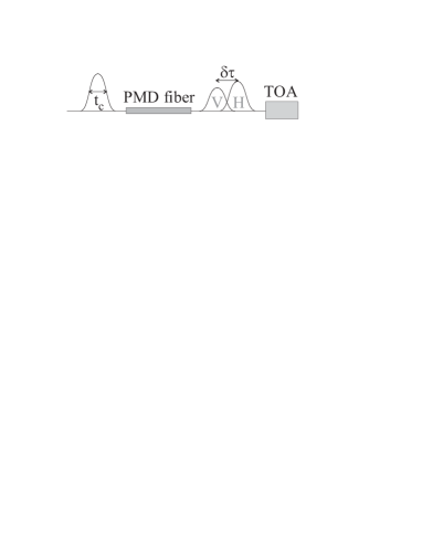
FIG. 1.: When a polarized pulse passing through a PMD fiber, the P-mode $H$ (parallel to the birefringency axis in the Poincar sphere) and its orthogonal $V$ are separated in time. A measurement of the time-of-arrival (TOA) is a measurement, strong or weak, of the polarization.

The first piece of the connection we want to point out is the following: a PMD element performs a measurement of polarization on light pulses (Fig. 1). In fact, PMD leads to the separation of two orthogonal P-modes in time; this separation is called differential group delay (DGD), noted $\delta\tau$. If $\delta\tau$ is larger than the pulse width, the measurement of the time of arrival is equivalent to the measurement of polarization — PMD acts then as a ”temporal polarizing beam-splitter”. However, in the usual telecom regime $\delta\tau$ is much smaller than the pulse width. In this case, the time of arrival does not achieve a complete discrimination between two orthogonal P-modes anymore; but still, some information about the polarization of the input pulse is encoded in the modified temporal shape of the output pulse. We are in a regime of weak measurement of the polarization; we are going to show later that we recover indeed the notion of weak measurement of the quantum theorists, by measuring the mean time of arrival (that is, the ”center of mass” of the output pulse).

The second piece of the connection defines the role of PDL: a PDL element performs a post-selection of some polarization modes. Far from being an artificial ingredient, post-selection of some modes is the most natural situation in the presence of losses: one does always post-select those photons that have not been lost! This would be trivial physics if the losses were independent of any degree of freedom, just like random scattering; but in the case of PDL, the amount of losses depends on the meaningful degree of freedom, polarization. An infinite PDL, as we said above, would correspond to the post-selection of a precise P-mode (a pure state, in the quantum language); a finite PDL corresponds to post-selecting different P-modes with different probabilities (a mixed quantum state).

In summary: by tuning the PMD, we can move from weak to strong measurements of polarization; by tuning the PDL, we can study the post-selection of a pure or of a mixed state of polarization. This is the main result of this paper, that we are now going to present in mathematical terms.

It is convenient to use the formalism of two-dimensional Jones vectors, in which the description of classical polarization is identical to the quantum description of the spin $\frac{1}{2}$ [7]. Thus e.g. the three typical pairs of orthogonal polarizations — horizontal-vertical linear, diagonal linear, left-right circular — are described respectively by the eigenvectors of the Pauli matrices $\sigma_{z}$, $\sigma_{x}$ and $\sigma_{y}$. In this paper, we shall only need to define the eigenvectors of $\sigma_{z}$: $\sigma_{z}\mbox{$|H\rangle$}=\mbox{$|H\rangle$}$, $\sigma_{z}\mbox{$|V\rangle$}=-\mbox{$|V\rangle$}$. Any pure polarization state can be described as a superposition of these vectors, with complex coefficients, the state corresponding to the point $\hat{n}=(\theta,\varphi)$ on the Poincaré sphere being $\mbox{$|+\hat{n}\rangle$}=\cos\frac{\theta}{2}\mbox{$|H\rangle$}+\sin\frac{\theta}{2}e^{i\varphi}\mbox{$|V\rangle$}$.

On a monochromatic wave of frequency $\omega$, a PMD that separates the eigenvectors of $\sigma_{z}$ for a birefringency $b$ is represented by the operator [5]

PMD: $$U(b\omega,\hat{z})\,=\,e^{ib\omega\,\sigma_{z}/2}\,=\,\cos\frac{b\omega}{2}\leavevmode\hbox{1\normalsize\kern-3.30002pt1}+i\sin\frac{b\omega}{2}\sigma_{z}\,.$$ (1)

This is a unitary operation that describes a global rotation of the state of polarization around the $z$ axis of the Poincaré sphere. As for PDL: since the most and least attenuated states are always orthogonal, they can be written as the eigenstates of $\sigma_{n}=\hat{n}\cdot\vec{\sigma}$, where the direction $\hat{n}$ has a priori no link with the direction $\hat{z}$ of the birefringency axis. Neglecting a global attenuation, the PDL is represented by the operator [5]

PDL: $$F(\mu,\hat{n})\,=\,e^{\mu\,\sigma_{n}/2}\,=\,\cosh\frac{\mu}{2}\leavevmode\hbox{1\normalsize\kern-3.30002pt1}+\sinh\frac{\mu}{2}\sigma_{n}\,.$$ (2)

This is a non-unitary operator, sometimes called a filter; in the quantum theory, it appears also in the unambiguous discrimination of non-orthogonal quantum states [8]. It has been shown in Ref. [5] that any optical network can be modelled by an effective PMD followed by an effective PDL, that is, by an operator of the form $F(\mu,\hat{n})U(b,\hat{m})$. However, the study of the general case is involved because the effective parameters $\mu$, $\hat{n}$, $b$ and $\hat{m}$ depend of the optical frequency $\omega$ in a non-trivial way, leading to deformations in the shape of the light pulse. Thus, we focus initially on the simplest optical network, namely a PMD fiber followed by a PDL element.

The input state is a gaussian (Fourier-transform limited) light pulse of coherence time $t_{c}$, of central frequency $\omega_{0}$, prepared in a pure polarization state $|\psi_{0}\rangle$:

$$|\Psi_{in}\rangle = {\cal A}\,e^{-\frac{1}{4}\left(\frac{t}{t_{c}}\right)^{2}}e^{-i\omega_{0}t}\otimes(\alpha\mbox{$|H\rangle$}+\beta\mbox{$|V\rangle$})$$ (3)

$$= g(t)\otimes\mbox{$|\psi_{0}\rangle$}\,,$$ (4)

with ${\cal A}=\big{(}\sqrt{2\pi}\,t_{c}\big{)}^{-1/2}$ so that $G(t)\equiv|g(t)|^{2}$ is a probability distribution [9]. To compute the state of the light at the output of the PMD fiber, we must Fourier-transform $|\Psi_{in}\rangle$ into the frequency domain, apply (1) to any monochromatic component, and integrate back to the time domain. This gives [10]

$$|\Psi_{PMD}\rangle = \int d\omega\,e^{-i\omega t}\tilde{g}(\omega-\omega_{0})\,U(b\omega,\hat{z})\mbox{$|\psi_{0}\rangle$}\,=$$ (5)

$$= \tilde{\alpha}\,g_{-}(t)\mbox{$|H\rangle$}+\tilde{\beta}\,g_{+}(t)\mbox{$|V\rangle$}$$ (6)

where $g_{\pm}(t)\equiv g(t\pm\frac{\delta\tau}{2})$ with $\delta\tau=b$, $\tilde{\alpha}=\alpha e^{ib\omega_{0}/2}$ and $\tilde{\beta}=\beta e^{-ib\omega_{0}/2}$. We see that, in addition to the global rotation around the birefringency axis at the frequency $\omega_{0}$, the PMD has delayed the $V$ polarization with respect to the $H$ polarization, as announced. According to whether the delay $\delta\tau$ is much larger or much smaller than the width $t_{c}$ of the input pulse, the recording of the time of arrival will provide us with a strong or a weak measurement [11]. For further reference, let us define the polarization state

$$|\psi\rangle = U(b\omega_{0},\hat{z})\mbox{$|\psi_{0}\rangle$}\,=\,\tilde{\alpha}\mbox{$|H\rangle$}+\tilde{\beta}\mbox{$|V\rangle$}$$ (7)

obtained by retaining only the global rotation, that is, in the limit of continuous light $\delta\tau/t_{c}\approx 0$.

Now, we should apply the PDL operator (2) to $|\Psi_{PMD}\rangle$. Before presenting the general case, to become familiar with the concepts, we study the case of post-selection of a pure state: the PDL element is then a polarizer that projects onto a polarization state $\mbox{$|\psi_{1}\rangle$}=\mu\mbox{$|H\rangle$}+\nu\mbox{$|V\rangle$}$. Thus, at the output of the optical network we have

$$|\Psi_{out}\rangle = \big{[}\tilde{\alpha}\bar{\mu}g_{-}(t)+\tilde{\beta}\bar{\nu}\,g_{+}(t)\big{]}\mbox{$|\psi_{1}\rangle$}\,\equiv\,F(t)\mbox{$|\psi_{1}\rangle$}\,,$$ (8)

where $\bar{z}$ is the conjugate of a complex number $z$. Clearly $F(t)$ is the temporal shape of the selected component of the field. Now we measure the intensity $I(t)=|F(t)|^{2}$; with $A=\tilde{\alpha}\bar{\mu}$ and $B=\tilde{\beta}\bar{\nu}$, we have

$$I(t) = |A|^{2}G_{-}(t)+|B|^{2}G_{+}(t)+2\mbox{Re}(\bar{A}B)g_{-}(t)g_{+}(t)\,.$$ (9)

In the limit of strong measurement, $\delta\tau>>t_{c}$, the overlap $g_{-}g_{+}$ is essentially 0, so the detected intensity corresponds to two well-separated gaussians: $I(t)=|\alpha\,\mu|^{2}\,G_{-}(t)\,+\,|\beta\,\nu|^{2}\,G_{+}(t)$. A detection in $G_{-}$ corresponds to the $H$ polarization, so the probability that the polarization was $|H\rangle$ given the preparation and post-selection is simply the integral of the gaussian $G_{-}$, normalized to the total intensity: $P(H)=\left(\int_{0}^{\infty}I(t)dt\right)/\left(\int_{-\infty}^{\infty}I(t)dt\right)\,=\,\frac{|\alpha\,\mu|^{2}}{|\alpha\,\mu|^{2}\,+\,|\beta\,\nu|^{2}}$. But $|\alpha|^{2}$ is the probability $P(H|\psi_{0})$ of finding a photon polarized along $|H\rangle$ given that the state is $|\psi_{0}\rangle$; using similar notations for $|\beta|^{2}$, $|\mu|^{2}$ and $|\nu|^{2}$, we have found

$$P(H) = \frac{P(\psi_{1}|H)P(H|\psi_{0})}{\sum_{K=H,V}P(\psi_{1}|K)P(K|\psi_{0})}.$$ (10)

This is the Aharonov-Bergmann-Lebowitz (ABL) rule [12], which corresponds to the classical rule for the probability of sequential events.

Since we have access to both $P(H)$ and $P(V)$, we can compute $\langle\sigma_{z}\rangle=P(H)-P(V)$. Moreover, the mean time-of-arrival, defined as usual by $\langle t\rangle=\left(\int tI(t)dt\right)/\left(\int I(t)dt\right)$, is here $P(H)\frac{\delta\tau}{2}+P(V)\big{(}-\frac{\delta\tau}{2}\big{)}$. So, for the case of strong measurement, we have derived the relation

$$\langle t\rangle = \frac{\delta\tau}{2}\,\langle\sigma_{z}\rangle\,.$$ (11)

This is the relation, that appears in any measurement theory, between the pointer or meter (here, the mean time of arrival) and physical quantity to be measured (here, $\sigma_{z}$). Even though it has been derived from more intuitive grounds in the regime of strong measurements, the relation (11) is the fundamental relation of a measurement process in which the coupling between the pointer and the observable quantity is made by the PMD [11]. In particular, contrary to $P(H)$ and $P(V)$, $\langle t\rangle$ can be defined and measured for any $I(t)$. We shall then take (11) as the definition of the mean value of $\sigma_{z}$ when measured by the PMD. With this, we can remove the assumption of strong measurement.

For $F(t)$ defined in (8), $\langle t\rangle$ can be calculated analytically. In fact, starting with $I(t)$ given by (9), a straightforward calculation and the relation (11) yield

$$\langle\sigma_{z}\rangle = \frac{|A|^{2}-|B|^{2}}{|A|^{2}+|B|^{2}+2Re(\bar{A}B)\,e^{-\frac{1}{2}({\delta\tau}/{2t_{c}})^{2}}}\,.$$ (12)

Note that the dependance in the strength of the measurement (i.e. in $\delta\tau/2t_{c}$) is very explicit in (12). In the limit of strong measurement, $\delta\tau/2t_{c}\rightarrow\infty$, we recover the above results. In the opposite limit, $e^{-\frac{1}{2}({\delta\tau}/{2t_{c}})^{2}}=1-O(\delta\tau/2t_{c})$, corresponding to a weak measurement, we have $\langle\sigma_{z}\rangle_{w}=\mbox{Re}\big{(}\frac{A-B}{A+B}\big{)}$. Noticing that

$$A\pm B\,=\,\tilde{\alpha}\bar{\mu}\pm\tilde{\beta}\bar{\nu} = \left\{\begin{array}[]{l}\mbox{$\langle\psi_{1}|\psi\rangle$}\\ \mbox{$\langle\psi_{1}|$}\sigma_{z}\mbox{$|\psi\rangle$}\end{array}\right.$$ (15)

with $|\psi\rangle$ given in (7), we find

$$\langle\sigma_{z}\rangle_{w}=\mbox{Re}\Big{(}\frac{\mbox{$\langle\psi_{1}|$}\sigma_{z}\mbox{$|\psi\rangle$}}{\mbox{$\langle\psi_{1}|\psi\rangle$}}\Big{)}\,.$$ (16)

This is exactly the formula for the weak value of $\sigma_{z}$ when the post-selection is done on a pure state $|\psi_{1}\rangle$ as given by the quantum theorists [1, 2]. Note in particular that $\langle\sigma_{z}\rangle_{w}$ can reach arbitrarily large values, leading to an apparently paradoxical situation since the eigenvalues of $\sigma_{z}$ are $\pm 1$. But there is no paradox at all: $\langle\sigma_{z}\rangle_{w}>1$ simply means $\langle t\rangle>\frac{\delta\tau}{2}$, and this situation is reached by post-selecting a state $|\psi_{1}\rangle$ that is almost orthogonal to $|\psi\rangle$; these are very rare events, the shape $F(t)$ of the pulse is strongly distorted, and it is not astonishing that its ”center of mass” could be found far away from its expected position in the absence of post-selection.

We can now examine the case of a finite value of the PDL after the PMD fiber. For conciseness, we write $F(\mu,\hat{n})\equiv F$ for the PDL operator (2). At the output of the PMD-PDL trunk, the state is

$$|\Psi_{out}\rangle = F\mbox{$|\Psi_{PMD}\rangle$}\,=\,A(t)\mbox{$|H\rangle$}+B(t)\mbox{$|V\rangle$}$$ (17)

where

$$A(t) = \mbox{$\langle H|F|H\rangle$}\,\tilde{\alpha}g_{-}(t)\,+\,\mbox{$\langle H|F|V\rangle$}\,\tilde{\beta}g_{+}(t)\,=$$ (18)

$$= \left(C+n_{z}S\right)\,\tilde{\alpha}g_{-}(t)\,+\,Sn_{-}\,\tilde{\beta}g_{+}(t)$$ (19)

$$B(t) = \mbox{$\langle V|F|V\rangle$}\,\tilde{\beta}g_{+}(t)\,+\,\mbox{$\langle V|F|H\rangle$}\,\tilde{\alpha}g_{-}(t)\,=$$ (20)

$$= \left(C-n_{z}S\right)\,\tilde{\beta}g_{+}(t)\,+\,Sn_{+}\,\tilde{\alpha}g_{-}(t)$$ (21)

with $C\equiv\cosh\frac{\mu}{2}$, $S\equiv\sinh\frac{\mu}{2}$ and $n_{\pm}=n_{x}\pm in_{y}$. We can then calculate the detected intensity $I(t)=|A(t)|^{2}+|B(t)|^{2}=|\alpha|^{2}(\cosh\mu+n_{z}\sinh\mu)G_{-}\,+\,|\beta|^{2}(\cosh\mu-n_{z}\sinh\mu)G_{+}\,+\,2\sinh\mu{\cal{R}}g_{+}g_{-}$ with ${\cal R}=\mbox{Re}\big{(}\alpha\bar{\beta}n_{+}e^{ib\omega_{0}}\big{)}$. The mean time of arrival is then calculated; with $\gamma=\tanh\mu$, the result is

$$\langle t\rangle = \frac{\delta\tau}{2}\,\frac{|\alpha|^{2}-|\beta|^{2}+\gamma\,n_{z}}{1+\gamma\big{[}n_{z}(|\alpha|^{2}-|\beta|^{2})+2{\cal R}\,e^{-\frac{1}{2}({\delta\tau}/{2t_{c}})^{2}}\big{]}}\,.$$ (22)

Again, in the limit of weak measurement and using (11), we find

$$\langle\sigma_{z}\rangle_{w} = \frac{\langle\sigma_{z}\rangle_{\psi}+\gamma\,n_{z}}{1+\gamma\,\vec{n}\cdot\langle\vec{\sigma}\rangle_{\psi}}\,=\,\mbox{Re}\left(\frac{\langle F^{\dagger}F\,\sigma_{z}\rangle_{\psi}}{\langle F^{\dagger}F\rangle_{\psi}}\right)$$ (23)

with $|\psi\rangle$ given by (7) as before. The r.h.s. is the weak value obtained by post-selection on the mixed state $\rho=\frac{1}{\mbox{Tr}(F^{\dagger}F)}F^{\dagger}F$ [2, 3]. The limiting case $\gamma=0$ means $\mu=0$, thence $\rho=\frac{1}{2}\leavevmode\hbox{1\normalsize\kern-3.30002pt1}$: if there is no PDL, $\langle\sigma_{z}\rangle_{w}=\langle\sigma_{z}\rangle_{\psi}$ as it should. At the other extreme, $\gamma=1$ means $\mu\rightarrow\infty$ thence $\rho=\frac{1}{2}(\leavevmode\hbox{1\normalsize\kern-3.30002pt1}+\sigma_{n})$, and we recover the formula (16) for the post-selection of the pure state $\mbox{$|\psi_{1}\rangle$}=\mbox{$|+\hat{n}\rangle$}$. Finally, we stress that the principal states of polarization of the PMD-PDL network, as defined e.g. in Ref. [5], are $F\mbox{$|H\rangle$}$ and $F\mbox{$|V\rangle$}$ [13].

We have then demonstrated our claims: an optical PMD-PDL network is an everyday realization of the abstract notions of weak measurement and post-selection introduced in the theory of quantum measurement. We had also said that telecom engineers would benefit by learning some quantum formalism, were it only because it could simplify their calculations. Indeed, consider a more complicated optical network, composed of three trunks: PMD-PDL-PMD, represented by the operator $T=U(b_{2}\omega,\hat{m})F(\mu,\hat{n})U(b_{1}\omega,\hat{z})$. As we noticed above, this simple network is sufficiently complex to yield anomalous dispersion. The calculation can of course be done following the same steps as above, but it is heavy and not really instructive. Another approach, that is moreover scalable to any network consisting of $2N+1$ trunks alternating PMD and PDL, is possible if the two PMD’s are weak, that is, in the telecom limit where the DGD’s $\delta\tau_{k}=b_{k}$ are much smaller than the width $t_{c}$ of the pulse; for conciseness, we write $\varepsilon=\tau_{k}/t_{c}$. This means that $\tilde{g}(\omega)=\tilde{g}(\omega_{0}+x)$ is significantly different from zero only for $|x|\leq\frac{1}{t_{c}}$, that is, $b_{k}x=O(\varepsilon)$. So we can expand all the PMD operators (1) as [10]

$$U(b\,\omega,\hat{m}) = \big{[}\leavevmode\hbox{1\normalsize\kern-3.30002pt1}+i(b\,x/2)\sigma_{m}+O(\varepsilon^{2})\big{]}\,U(b\,\omega_{0},\hat{m})\,.$$ (24)

Let us then calculate the three-trunk network:

$$T(x) \simeq {\cal{F}}\,+\,i\,x\,\Big{(}\frac{b_{1}}{2}{\cal{F}}\sigma_{z}+\frac{b_{2}}{2}\sigma_{m}{\cal{F}}\Big{)}\,+\,O(\varepsilon^{2})$$ (25)

with ${\cal{F}}=U(b_{2}\,\omega_{0},\hat{m})FU(b_{1}\,\omega_{0},\hat{z})$. In what follows, we define the two orthogonal states of polarization $\mbox{$|\psi_{F}\rangle$}={\cal{F}}\mbox{$|\psi_{0}\rangle$}/\sqrt{\langle{\cal{F}}^{\dagger}{\cal{F}}\rangle_{\psi_{0}}}$ and $|\psi_{F}^{\perp}\rangle$, and we systematically omit global attenuations. We have:

$$T(x)\mbox{$|\psi_{0}\rangle$} = {\mbox{$\langle\psi_{F}|T|\psi_{0}\rangle$}}\mbox{$|\psi_{F}\rangle$}\,+\,{\mbox{$\langle\psi_{F}^{\perp}|T|\psi_{0}\rangle$}}\mbox{$|\psi_{F}^{\perp}\rangle$}$$ (26)

$$\propto \big{(}1+i\,x\,W\big{)}\,\mbox{$|\psi_{F}\rangle$}\,+\,x\,C\,\mbox{$|\psi_{F}^{\perp}\rangle$}\,+O(\varepsilon^{2})\,,$$ (27)

where $W=\mbox{$\langle\psi_{0}|$}{\cal{F}}^{\dagger}\big{(}\frac{b_{1}}{2}{\cal{F}}\sigma_{z}+\frac{b_{2}}{2}\sigma_{m}{\cal{F}}\big{)}\mbox{$|\psi_{0}\rangle$}/\langle{\cal{F}}^{\dagger}{\cal{F}}\rangle_{\psi_{0}}$ and $xC\sim O(\varepsilon)$. The passage from the Fourier to the time domain yields

$$|\Psi_{3}\rangle = \int dxe^{-i(x+\omega_{0})t}\,\tilde{g}(x)\,\otimes T(x)\,\mbox{$|\psi_{0}\rangle$}$$ (28)

$$\propto g\big{(}t-\mbox{Re}(W)\big{)}e^{-i\omega_{0}t}\otimes\mbox{$|\psi_{F}\rangle$}\,+\,h(t)\otimes\mbox{$|\psi_{F}^{\perp}\rangle$}$$ (29)

where we used $1+ixW=e^{ixW}+O(\varepsilon^{2})$ and where $h(t)\sim O(\varepsilon)$. The measurement of the intensity of the light pulse $|\Psi_{3}\rangle$ gives $I(t)\,\propto\,G\big{(}t-\mbox{Re}(W)\big{)}+O(\varepsilon^{2})$: the center of the pulse is now in

$$\langle t\rangle = \mbox{Re}(W)\,=\,\frac{b_{1}}{2}\,w_{1}\,+\,\frac{b_{2}}{2}\,w_{2}$$ (30)

with $w_{1}$ given by (23) and $w_{2}=\mbox{$\langle\psi_{F}|\sigma_{m}|\psi_{F}\rangle$}$. This result is intuitively clear: the first term is the weak value obtained by forgetting the second PMD element; the second term is just the mean value of $\sigma_{m}$ on the filtered state obtained by forgetting the first PMD element. For the case of any network composed of $2N+1$ trunks alternating PMD and PDL elements, the result generalizes immediately as $\langle t\rangle=\sum_{k}\frac{\delta\tau_{k}}{2}\,w_{k}$, with $w_{k}$ the suitable weak values [13]. This example shows how the formalism of weak measurements simplifies some calculations of networks combining PMD and PDL, adding an intuitive meaning to the formulae.

In conclusion, we have shown that the quantum theoretical formalism of weak measurements and post-selection, often thought of as a weirdness of theorists, describes important effects in the physics of telecom fibers. In particular, the notion of post-selection appears naturally, since the telecom engineers select only those photons that are not lost in the fiber.

Just a final remark, to say that, with this investigation, we close a loop of analogies. On the one hand, in Ref. [14], Gisin and Go stressed the analogy between the PMD-PDL effects in optical networks and the mixing and decay of kaons. On the other hand, in Ref. [15] it was shown that adiabatic measurements in metastable systems are a kind of weak measurement, and point out that kaons provide experimental examples of this. By showing the link between PMD-PDL and weak measurements with post-selection, this work closes the loop.

REFERENCES

- [1] Y. Aharonov, D. Albert, L. Vaidman, Phys. Rev. Lett. 60, 1351 (1988)
- [2] Y. Aharonov, L. Vaidman, quant-ph/0105101 (2001); published in: J. G. Muga, R. Sala Mayato and I. L. Egusquiza (eds), Time in Quantum Mechanics, Lecture Notes in Physics, (Springer Verlag, 2002).
- [3] A.M. Steinberg, quant-ph/0302003 (2003).
- [4] The possibility of testing the theory of weak values with linear optics and polarization has been exploited in: N.W.M. Ritchie, J.G. Story, R.G. Hulet, Phys. Rev. Lett. 66, 1107 (1991); D. Suter, Phys. Rev. A 51, 45 (1995).
- [5] B. Huttner, C. Geiser, N. Gisin, IEEE J. Sel. Top. Quant. Electron. 6, 317 (2000)
- [6] P. Lu, L. Chen, X.Y. Bao, J. Lightwave Technol. 19, 856 (2001)
- [7] See any treatise on the polarization of light, e.g. S. Huard, Polarisation de la lumière (Masson, Paris, 1994); transl: Polarization of light (Wiley, New York, 1997)
- [8] A. Peres, Quantum Theory: Concepts and Methods (Kluwer, Dordrecht, 1998), section 9-5; B. Huttner et al., Phys. Rev. A 54, 3783 (1996)
- [9] The ”time” in our equations is not the evolution parameter alone, but should rather be , where is the position in the fiber and is the average light speed in the fiber. That is why quantum theorists can well consider as a ”position” and as its conjugate ”momentum”.
- [10] Note that .
- [11] Note that the PMD alone is a reversible operation: the simple fact of delaying one polarization mode is not a complete measurement — it is sometimes called a pre-measurement.
- [12] Y. Aharonov, P.G. Bergmann, J.L. Lebowitz, Phys. Rev. B 134, 1410 (1964)
- [13] N. Brunner, diploma thesis, University of Geneva, 2003
- [14] N. Gisin, A. Go, Am. J. Phys. 69, 264 (2001)
- [15] Y. Aharonov, S. Massar, S. Popescu, J. Tollaksen, L. Vaidman, Phys. Rev. Lett. 77, 983 (1996)