Quantum Dynamics of the Oscillating Cantilever-Driven Adiabatic Reversals in Magnetic Resonance Force Microscopy

Abstract

We simulated the quantum dynamics for magnetic resonance force microscopy (MRFM) in the oscillating cantilever-driven adiabatic reversals (OSCAR) technique. We estimated the frequency shift of the cantilever vibrations and demonstrated that this shift causes the formation of a Schrödinger cat state which has some similarities and differences from the conventional MRFM technique which uses cyclic adiabatic reversals of spins. The interaction of the cantilever with the environment is shown to quickly destroy the coherence between the two possible cantilever trajectories. We have shown that using partial adiabatic reversals, one can produce a significant increase in the OSCAR signal.

I Introduction

The oscillating cantilever-driven adiabatic reversals (OSCAR) technique is, probably, the most promising way to achieve single-spin detection using magnetic resonance force microscopy (MRFM) 1 ; 2 . In the OSCAR technique, the oscillating cantilever produces an oscillating $z$-component of the effective magnetic field in the system of coordinates connected to the rotating rf field, which causes the magnetic moment reversals. In turn, the cyclic adiabatic reversals of the magnetic moment cause the frequency shift in the cantilever vibrations, which is to be measured.

While the classical dynamics of the OSCAR has been studied in 1 ; 2 , the quantum dynamics has never been investigated. This paper describes the quantum dynamics of the spin-cantilever system in the OSCAR technique. In Section 2, we introduce the quantum Hamiltonian and the equations of motion for the system. In Section 3, we present a qualitative analysis and estimates of the OSCAR signal. We show that the OSCAR signal can be increased by sacrificing the full reversals of the effective field. Namely, partial adiabatic reversals can provide a larger signal than the full reversals. We estimate the maximum OSCAR signal generated by a single spin. In Section 4, we present numerical simulations of quantum dynamics using the Schrödinger equation. In particular, we demonstrate the formation of a Schrödinger cat state which simultaneously includes two possible trajectories of the cantilever. In Section 5, we present numerical simulations of the decoherence caused by the interaction of the cantilever with the thermal environment.

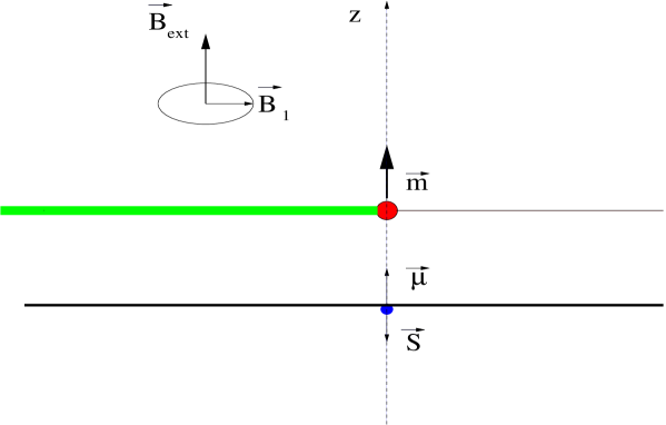
Figure 1: The geometry of the OSCAR MRFM. ${\vec{m}}$ is the magnetic moment of the ferromagnetic particle on the cantilever tip; ${\vec{\mu}}$ and ${\vec{S}}$ are the magnetic moment and the spin of an atom (in the ground state); ${\vec{B}}_{ext}$ and ${\vec{B}}_{1}$ are the permanent and rotating magnetic fields.

II The Hamiltonian and equations of motion

We describe the cantilever interacting with a single electron spin 1/2 as a harmonic oscillator with the fundamental frequency $\omega_{c}$. The dimensionless quantum Hamiltonian of this system can be written (in the rotating coordinate systems) as

$${\cal H}=\frac{1}{2}(p^{2}+z^{2})+\varepsilon S_{x}-2\eta zS_{z},$$

with the dimensionless parameters

$$p=P/P_{0},~{}z=Z/Z_{0},~{}\varepsilon=\gamma B_{1}/\omega_{c},~{}P_{0}=\hbar/Z_{0},$$

$$\eta=\gamma\hbar\Bigg{|}{{\partial B_{z}}\over{\partial z}}\Bigg{|}/2(\hbar\omega_{c}k_{c})^{1/2},~{}Z_{0}=(\hbar\omega_{c}/k_{c})^{1/2}.$$

Here $P$ and $Z$ are operators of the momentum and the $z$-coordinate of the cantilever, $k_{c}$ is the cantilever spring constant, $B_{1}$ is the magnitude of the rotating magnetic field, $\gamma$ is the magnitude of the electron gyromagnetic ratio, $B_{z}$ is the $z$-component of the magnetic field acting on the spin, including the external permanent magnetic field $B_{ext}$ and the magnetic field produced by the ferromagnetic particle. (See Fig. 1.)

The quantum dynamics of the MRFM was studied earlier in 3 ; 4 . In these papers the oscillating $z$-component of the effective magnetic field acting on the spin was considered to be generated by frequency modulation of the external rotating field $B_{1}$. The $z$-component of the effective field, $-2\eta z$, associated with the cantilever vibrations, was negligible in comparison with the $z$-component of the external effective field. Below we consider the opposite (OSCAR) situation: the oscillating $z$-component of the effective field is produced by cantilever vibrations.

To simulate the Schrödinger dynamics, we use the dimensionless Schrödinger equation

$$i{{\partial\Psi}\over{\partial\tau}}={\cal H}\Psi,$$

where the wave function $\Psi$ is

$$\Psi=u_{\alpha}(z,\tau)\alpha+u_{\beta}(z,\tau)\beta,$$

$$\alpha=\left(\matrix{1\cr 0\cr}\right),~{}\beta=\left(\matrix{0\cr 1\cr}\right),~{}\tau=\omega_{c}t.$$

The orbital wave functions $u_{\alpha,\beta}(z,\tau)$ have been expanded in the eigenfunctions, $u_{n}(z)$, of the oscillator Hamiltonian with time-dependent coefficients. The resulting system of differential equations for time-dependent coefficients was solved for a finite set of basis functions $u_{n}(z)$. Alternatively, we have found eigenvalues and eigenvectors of the time-independent Hamiltonian ${\cal H}$ for the same finite basis, and constructed from them the time dependent solution. These two approaches have been shown to give the same results.

To simulate the decoherence process, we used the simplest master equation (an ohmic model in the high-temperature approximation 5 )

$${{\partial\rho_{s,s^{\prime}}}\over{\partial\tau}}=\Bigg{[}{{i}\over{2}}\Bigg{(}{{\partial^{2}}\over{\partial z^{2}}}-{{\partial^{2}}\over{\partial z^{\prime 2}}}\Bigg{)}-{{i}\over{2}}(z^{2}-z^{\prime 2})$$

$$-{{1}\over{2Q}}(z-z^{\prime})\Bigg{(}{{\partial}\over{\partial z}}-{{\partial}\over{\partial z^{\prime}}}\Bigg{)}-{{D}\over{Q}}(z-z^{\prime})^{2}$$

$$-2i\eta(z^{\prime}s^{\prime}-zs)\Bigg{]}\rho_{s,s^{\prime}}-i{{\varepsilon}\over{2}}(\rho_{s,-s^{\prime}}-\rho_{-s,s^{\prime}}),$$

where $\rho_{s,s^{\prime}}\equiv\rho_{s,s^{\prime}}(z,z^{\prime},\tau)$ is the density matrix, $s,s^{\prime}=\pm 1/2$, $D=k_{B}T/\hbar\omega_{c}$ is the dimensionless diffusion coefficient, and $Q$ is the quality factor of the cantilever.

The function $\rho_{s,s^{\prime}}(z,z^{\prime},\tau)$ was expanded in the basis of the eigenfunctions $u_{n}(z)u^{*}_{m}(z^{\prime})$ with time-dependent coefficients. These coefficients were calculated numerically for a finite set of basis functions.

III Qualitative analysis and estimates of the OSCAR signal

Suppose that initially a single spin is parallel to the effective magnetic field ${\vec{B}_{eff}}=(\varepsilon,0,-2\eta z)$. Under the conditions of adiabatic motion, the spin component along the effective magnetic field is an integral of motion. Thus, in the process of motion the spin will have the same definite direction relative to the effective magnetic field. Consequently, the orbital and spin degrees of freedom are not entangled: the wave function of the system will remain a tensor product of the orbital and spin parts. As a result, the spin-cantilever correlators are equal to zero, and the Heisenberg equations of motion

$$\dot{z}=p,~{}\dot{p}=-z+2\eta S_{z},$$

$$\dot{S}_{x}=2\eta zS_{z},~{}\dot{S}_{y}=-2\eta zS_{x}-\varepsilon S_{z},~{}\dot{S}_{z}=\varepsilon S_{y},$$

are equivalent to the classical equations of motion. That is why in this case we can use classical estimates for the single-spin OSCAR signal.

We estimate the OSCAR signal in the following way: under the conditions of adiabatic motion (and if the spin is parallel to the effective field) we have

$$S_{z}/S=\mp B_{eff}^{z}/B_{eff},$$

where the upper sign corresponds to the ground state (the spin points in the direction opposite to the direction of the effective field). It follows from Eq. (7) that

$$S_{z}=\pm{{\eta z}\over{\sqrt{(2\eta z)^{2}+\varepsilon^{2}}}}.$$

Now, we substitute this expression into the equation for the cantilever coordinate $z$

$$\ddot{z}+z-2\eta S_{z}=0.$$

Neglecting oscillations with twice the cantilever frequency, we have from Eqs. (8) and (9)

$$\ddot{z}+z\mp{{2\eta^{2}z}\over{\sqrt{2\eta^{2}z_{m}^{2}+\varepsilon^{2}}}}=0,$$

where $z_{m}$ is the amplitude of the cantilever vibrations. Assuming that the cantilever frequency shift $\Delta\omega_{c}$ is small in comparison to the unperturbed cantilever frequency, $\omega_{c}$, $(|\Delta\omega_{c}|\ll\omega_{c})$ we have the estimate for the OSCAR signal:

$${{\Delta\omega_{c}}\over{\omega_{c}}}=\mp{{\eta^{2}}\over{\sqrt{2\eta^{2}z^{2}_{m}+\varepsilon^{2}}}}.$$

Note that the frequency shift (11) decreases with increasing of the cantilever amplitude $z_{m}$. The reason for this dependence is the following. The frequency shift is associated with the restoring spin force $F_{s}\propto z$. Roughly speaking, the OSCAR signal is determined by the ratio $F_{sm}/z_{m}$, where $F_{sm}$ is the maximum spin force. When $z_{m}$ increases, the value $F_{sm}$ approaches its limit $\eta$ (in dimensionless notation). Thus, the ratio $F_{sm}/z_{m}$ decreases.

As an example, we estimate the single-spin signal for the experimental parameters in 1 :

$$k_{c}=0.014{\rm N/m},~{}\omega_{c}/2\pi=21.4{\rm kHz},~{}Z_{m}=28{\rm nm},$$

$$~{}\Bigg{|}{{\partial B_{z}}\over{\partial z}}\Bigg{|}=1.4\times 10^{5}{\rm T/m},~{}B_{1}=0.3{\rm mT}.$$

Using Eq. (2) we obtain

$$\eta=2.9\times 10^{-3},~{}z_{m}=8.8\times 10^{5},~{}\varepsilon=390.$$

It follows from Eq. (11) that the relative cantilever frequency shift is $|\Delta\omega_{c}|/\omega_{c}=2.3\times 10^{-9}$.

The condition for the adiabatic motion in terms of the dimensionless parameters can be written as

$$2\eta z_{m}\ll\varepsilon^{2}.$$

To provide the full reversals of the effective field one also requires

$$\varepsilon\ll 2\eta z_{m}.$$

As an example, in the experiment 1 we have: $2\eta z_{m}=5.2\times 10^{3}$, $\varepsilon^{2}=1.5\times 10^{5}$. Thus, both inequalities (14) and (15) are satisfied, i.e. we have full adiabatic reversals.

Next, we discuss a way to increase the OSCAR signal. It follows from Eq. (11) that one should sacrifice the requirement for the full reversals (15) and reduce the amplitude of the cantilever vibrations $z_{m}$ and the amplitude of the rf field $\varepsilon$, in order to increase the frequency shift. The minimum possible dimensional cantilever amplitude can be estimated as

$$Z_{m}\sim Z_{rms}=\sqrt{k_{B}T/k_{c}}.$$

As an example, in the experiment 1 , for $T=3$K, the minimum value of $z_{m}$ is $1.72\times 10^{3}$. Thus, the $z$-component of the effective field, $2\eta z_{m}=10$. Taking $\varepsilon=2\eta z_{m}$, we still satisfy the adiabatic condition (14) but clearly violate the condition (15) for full reversals. In this case, $\Delta\omega_{c}/\omega_{c}=7\times 10^{-7}$, and is 300 times greater than for the experimental parameters (13).

The OSCAR signal should be compared with the frequency thermal noise $\delta\omega_{c}/\omega_{c}$. To estimate this noise we assume that the noise force changes from zero to its rms value $F_{rms}$ while the $z$-coordinate of the cantilever tip changes from zero to $Z_{m}$. Then the effective change of the cantilever spring constant is $\delta k_{c}=F_{rms}/Z_{m}$. Using the expression $\omega_{c}^{2}=k_{c}/m^{*}$, where $m^{*}$ is the effective cantilever mass, we obtain

$${{\delta\omega_{c}}\over{\omega_{c}}}={{\delta k_{c}}\over{2k_{c}}}={{F_{rms}}\over{2k_{c}Z_{m}}}.$$

Finally, using the well-known estimate for $F_{rms}$ (see, for example, 6 )

$$F_{rms}=2(k_{B}Tk_{c}B/Q\omega_{c})^{1/2},$$

where $B$ is the measurement bandwidth, we derive the estimate for the frequency thermal noise

$${{\delta\omega_{c}}\over{\omega_{c}}}=(Z_{m})^{-1}(k_{B}TB/k_{c}\omega_{c}Q)^{1/2}.$$

(This estimate was derived in 7 , using a different approach.) For the “natural” measurement bandwidth, $B=\omega_{c}/4Q$, we have from Eq. (19)

$${{\delta\omega_{c}}\over{\omega_{c}}}=(2QZ_{m})^{-1}(k_{B}T/k_{c})^{1/2}.$$

Taking parameters (12) and $T=3$K, $Q=10^{4}$, we find $\delta\omega_{c}/\omega_{c}\approx 9.7\times 10^{-8}$, which is smaller than the estimated OSCAR signal, $\Delta\omega_{c}/\omega_{c}=7\times 10^{-7}$.

Note, that the thermal noise is inversely proportional to the cantilever amplitude $Z_{m}$. Thus, the amplification of the OSCAR signal, associated with a decrease of $Z_{m}$, does not assume an increase of the signal-to-noise ratio. However, the decrease of the field amplitude, $B_{1}$, which becomes possible for small values of $Z_{m}$, would result in reducing the cantilever heating, which is an important obstacle for a single-spin detection.

So far, we did not discuss the quantum effects in OSCAR. These effects appear if the initial average spin is not parallel to the effective field. In the classical case, the angle $\theta$ between the effective field and the magnetic moment is an integral of motion. The estimated classical frequency shift

$$\Delta\omega_{c}/\omega_{c}=-{{\eta^{2}\cos\theta}\over{\sqrt{2\eta^{2}z_{m}^{2}+\varepsilon^{2}}}},$$

will approach zero as $\theta$ approaches $\pi/2$. In the quantum case, we expect to obtain one of two possible values in (11) independent of the initial angle $\theta$. This outcome corresponds to the standard Stern-Gerlach effect.

IV Simulations of quantum dynamics

In our simulations we used the following values of parameters

$$\eta=0.3,~{}z_{m}=13,~{}\varepsilon=10.$$

For the cantilever used in 1 this value of $\eta$ corresponds to a magnetic field gradient of $1.4\times 10^{7}$ T/m, and the value of $z_{m}$ corresponds to the temperature below $170$$\mu K$.

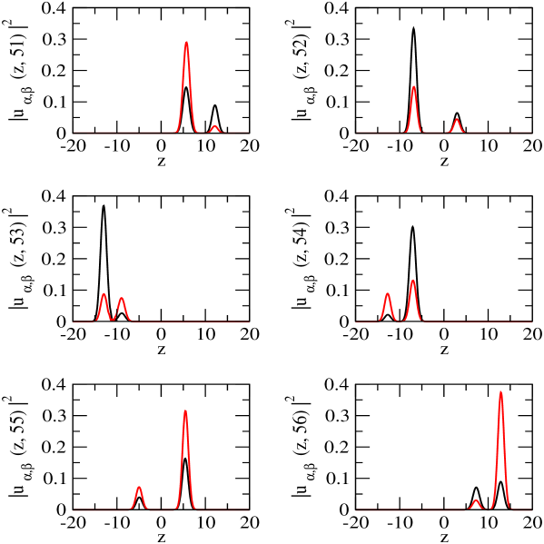
Figure 2: Functions $|u_{\alpha}(z,\tau)|^{2}$ (black curve) and $|u_{\beta}(z,\tau)|^{2}$ (red curve), for six values of $\tau$. Initial conditions: $\langle z(0)\rangle=z_{m}=13$, $\langle p(0)\rangle=0$, and the electron spin points in the positive $z$-direction.

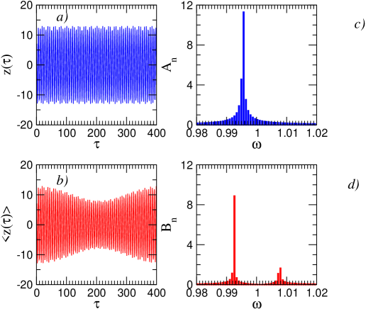
Figure 3: Classical and quantum cantilever dynamics in OSCAR MRFM; (a) classical cantilever coordinate $z(\tau)$, (b) quantum average cantilever coordinate $\langle z(\tau)\rangle$, (c) the Fourier spectrum for (a): $z(\tau)=\sum_{n}A_{n}\cos(\omega_{n}\tau+\varphi_{n})$, (d) the Fourier spectrum for (b): $\langle z(\tau)\rangle=\sum_{n}B_{n}\cos(\omega_{n}\tau+\theta_{n})$. All parameters are the same as in Fig. 2. In a) and b) we show, for convenience, time sequences shorter than those used in order to get the Fourier spectrum shown in c) and d).

These parameters allow us to reduce the computational time. The maximum value of the $z$-component of the effective field is, $2\eta z_{m}=7.8$. Thus, the condition (14) of adiabatic motion is satisfied while the condition (15) for full reversals is clearly violated. The estimated frequency shift is: $|\Delta\omega_{c}|/\omega_{c}=7.9\times 10^{-3}$.

The initial conditions which we used correspond to the quasiclassical state of the cantilever, and the electron spin pointing in the positive $z$-direction. That means, in Eqs. (4), $u_{\beta}(z,0)=0$ and,

$$u_{\alpha}(z,0)=\sum_{n=0}^{\infty}\pi^{1/4}2^{n/2}\alpha_{0}^{n}H_{n}(z)\exp[-(z^{2}+|\alpha_{0}|^{2})/2],$$

where $H_{n}(z)$ is a Hermitian polynomial, and

$$\alpha_{0}=(\langle z(0)\rangle+i\langle p(0)\rangle)/\sqrt{2},~{}\langle z(0)\rangle=13,~{}\langle p(0)\rangle=0.$$

Our simulations show that the probability distribution for the cantilever position

$$P(z,\tau)=|u_{\alpha}(z,\tau)|^{2}+|u_{\beta}(z,\tau)|^{2}$$

eventually splits into two peaks which describe two trajectories of the cantilever. The ratio of the integrated probabilities for two peaks is given approximately by $tan^{2}(\theta/2)$, where $\theta$ is the initial angle between the directions of the average spin and the effective field $\vec{B}_{eff}=(\varepsilon,0,-2\eta z(0))$. The approximate position of the center of the first peak is

$$z_{1}=z_{m}\cos(1-|\Delta\omega_{c}|/\omega_{c})\tau,$$

and the approximate position of the second peak is

$$z_{2}=z_{m}\cos(1+|\Delta\omega_{c}|/\omega_{c})\tau,$$

where $|\Delta\omega_{c}|/\omega_{c}\approx 8.0\times 10^{-3}$. (The value $|\Delta\omega_{c}|/\omega_{c}$ estimated from (11) is almost the same, $7.9\times 10^{-3}$.) Both functions $u_{\alpha}(z,\tau)$ and $u_{\beta}(z,\tau)$ contribute to each peak. (See Fig. 2.) When two peaks are clearly separated, the wave function $\Psi$ can be approximately represented as a sum of two functions $\Psi_{1}$ and $\Psi_{2}$, which correspond to two peaks in the probability distribution. We have found that each function $\Psi_{1}$ and $\Psi_{2}$, with the accuracy to 1%, can be represented as a product of the coordinate and spin functions

$$\Psi_{1}=R_{1}(z,\tau)\chi_{1}(\tau),~{}\Psi_{2}=R_{2}(z,\tau)\chi_{2}(\tau).$$

The first spin function $\chi_{1}(\tau)$ describes the average spin which points approximately opposite to the direction of the effective field $\vec{B}_{eff,1}=(\varepsilon,0,z_{1})$, for the first cantilever trajectory. The second spin function $\chi_{2}(\tau)$ describes the average spin which points approximately in the direction of the effective field $\vec{B}_{eff,2}=(\varepsilon,0,z_{2})$, for the second cantilever trajectory.

Unlike a conventional MRFM dynamics studied in 3 ; 4 the OSCAR technique implies different effective fields for two cantilever trajectories.

That is why, in general, the average spins corresponding to two cantilever trajectories do not point in the opposite directions, and the wave functions $\chi_{1}(\tau)$ and $\chi_{2}(\tau)$ are not orthogonal to each other. The only exceptions are the instants $\tau$ for which two cantilever trajectories intersect providing a unique direction for the effective field.

As we already mentioned, the frequency shift for two cantilever trajectories $\Delta\omega_{c}/\omega_{c}$ was found to be $\pm 8\times 10^{-3}$. For comparison, we solved the classical equations of motion with the same parameters and initial conditions as in the quantum case. The frequency shift for a single cantilever trajectory in the classical case was found to be $\Delta\omega_{c}/\omega_{c}=-5\times 10^{-3}$, which is smaller than the quantum shift and very close to the value $-5.3\times 10^{-3}$ derived from the estimate (20). (See Fig. 3.)

Figure 4: Evolution of the density matrix without the decoherence effects ($Q^{-1}=D=0$), for four instants of time (as indicated in the figure) . Parameters: $\varepsilon=10$, $\eta=0.3$. The left column: $\ln|\sum_{s}\rho_{s,s}|$, the right column: $\ln|\sum_{s}\rho_{s,-s}|$. Initial conditions: $\langle z(0)\rangle=-8$, $\langle p(0)\rangle=0$, and the electron spin points in the positive $z$-direction. Contour lines have been obtained by intersections of the functions $\ln|\sum_{s}\rho_{s,\pm s}|$ with horizontal planes at different heights $h$. Different colours indicates different regions in the following way : $h<-14$ (white) ,$-14<h<-12$ (black) , $-12<h<-10$ (red), $-10<h<-8$ (green) $-8<h<-6$ (blue) , $-6<h<-4$ (yellow), $h>-4$ (pink) .

V Decoherence of the Schrödinger cat state

To describe qualitatively the decoherence process, we solved numerically the master equation (5). The initial density matrix describes a pure quantum state with the quasiclassical cantilever and the spin oriented in the positive $z$-direction. At $\tau=0$ we have

$$\rho_{s,s^{\prime}}(z,z^{\prime},0)=u_{\alpha}(z,0)u^{*}_{\alpha}(z^{\prime},0)\left(\matrix{1&0\cr 0&0\cr}\right),$$

where the expression for $u_{\alpha}(z,0)$ is given in (22), and we put in (23) $\langle p(0)\rangle=0$, $\langle z(0)\rangle=-8$. Fig. 4 shows the evolution of the density matrix without effects of decoherence, for the following values of parameters

$$\varepsilon=10,~{}\eta=0.3,~{}Q^{-1}=D=0.$$

The left column demonstrates the behavior of the spin diagonal density matrix components (contour lines for $\ln|\sum_{s}\rho_{s,s}|)$, and the right column demonstrates the behavior of the spin non-diagonal density matrix components (contour lines for $\ln|\sum_{s}\rho_{s,-s}|)$. Initially we have one peak on the plane $z-z^{\prime}$. Eventually, this peak splits into four peaks. Two spatial diagonal peaks, which are centered on the line $z=z^{\prime}$, correspond to two cantilever trajectories. Two spatial non-diagonal peaks describe a “coherence” between the two trajectories, which is a quantitative characteristic of the Schrödinger cat state. All four spin components of the density matrix $\rho_{s,s^{\prime}}(z,z^{\prime},\tau)$ (with $s=\pm 1/2,s^{\prime}=\pm 1/2$) contribute to each peak in the $z-z^{\prime}$ plane.

The density matrix $\rho_{s,s^{\prime}}(z,z^{\prime},\tau)$ can be represented as a sum of four terms

$$\rho_{s,s^{\prime}}(z,z^{\prime},\tau)=\sum_{k=1}^{4}\rho^{(k)}_{s,s^{\prime}}(z,z^{\prime},\tau),$$

where each term describes one peak in the $z-z^{\prime}$ plane. Suppose that first two terms in (29) with $k=1,2$ describe the spatial diagonal peaks, and two other terms with $k=3,4$ describe the spatial non-diagonal peaks.

We have found that the diagonal terms $\rho^{(1)}$ and $\rho^{(2)}$ can be approximately decomposed into the tensor product of the coordinate and spin parts

$$\rho^{(k)}_{s,s^{\prime}}(z,z^{\prime},\tau)=\hat{R}^{(k)}(z,z^{\prime},\tau)\hat{\chi}^{(k)}_{s,s^{\prime}}(\tau),~{}k=1,2.$$

The spin matrix $\hat{\chi}^{(1)}_{s,s^{\prime}}(\tau)$ describes the average spin which points approximately opposite to the direction of the effective field $\vec{B}_{eff,1}$. The spin matrix $\hat{\chi}^{(2)}_{s,s^{\prime}}(\tau)$ describes the average spin which points approximately in the direction of the effective field $\vec{B}_{eff,2}$.

Figure 5: Evolution of the density matrix: effects of decoherence and thermal noise; $D=20$, $Q^{-1}=0.001$, $\varepsilon=10$, $\eta=0.3$. The left column: $\ln|\sum_{s}\rho_{s,s}|$, the right column: $\ln|\sum_{s}\rho_{s,-s}|$. Initial conditions: $\langle z(0)\rangle=-8$, $\langle p(0)\rangle=0$, and the electron spin points in the positive $z$-direction. Contour lines have been obtained by intersections of the functions $\ln|\sum_{s}\rho_{s,\pm s}|$ with horizontal planes at different heights $h$. Different colours indicates different regions in the following way : $h<-14$ (white) ,$-14<h<-12$ (black) , $-12<h<-10$ (red), $-10<h<-8$ (green) $-8<h<-6$ (blue) , $-6<h<-4$ (yellow), $h>-4$ (pink).

We have found that the same properties of the density matrix remain for the case $Q^{-1},D\not=0$. Fig. 5 demonstrates the effects of decoherence and thermal noise for $Q^{-1}=0.001$ and $D=20$. The spatial non-diagonal peaks in the $z-z^{\prime}$ plane quickly decay. This reflects the effect of decoherence: the statistical mixture of two possible cantilever trajectories replaces the Schrödinger cat state. Next, the spatial diagonal peaks spread out along the line $z=z^{\prime}$. This reflects the classical effect of the thermal diffusion.

Conclusion

We presented a quantum theory of the OSCAR MRFM technique. We demonstrated that the OSCAR signal can be significantly amplified by using partial reversals of the effective field instead of the full reversals. If the initial angle $\theta$ between the directions of the effective field and the average spin is not small, the quantum frequency shift remains constant, while the corresponding classical frequency shift is proportional to $\cos\theta$. This result is a manifestation of the Stern-Gerlach effect in the OSCAR MRFM.

Unlike the “conventional MRFM” in which the reversals of the effective field are provided by the frequency modulation of the rf field, the OSCAR MRFM exhibits two possible directions of the effective field. As a result, unlike the conventional MRFM, and the Stern-Gerlach effect, the two directions of the spin corresponding to two cantilever trajectories do not remain antiparallel to each other during the quantum evolution.

References

• (1) B.C. Stipe, H.J. Mamin, C.S. Yannoni, T.D. Stowe, T.W. Kenny, D. Rugar, Phys. Rev. Lett., 87, 277602 (2001).
• (2) G.P. Berman, D.I. Kamenev, V.I. Tsifrinovich, Phys. Rev. A, 66, 023405 (2002).
• (3) G.P. Berman, F. Borgonovi, G. Chapline, S.A. Gurvitz, P.C. Hammel, D.V. Pelekhov, A. Suter, V.I. Tsifrinovich, J. of Phys. A : Math. and General 36 4417 (2003).
• (4) G.P. Berman, F. Borgonovi, H.S. Goan, S.A. Gurvitz, V.I. Tsifrinovich, Phys. Rev. B 67, 094425 (2003).
• (5) Caldeira, A.J. Leggett, Physica A, 121, 587 (1987).
• (6) G.P. Berman, V.I. Tsifrinovich, Phys. Rev. B, 61, 3524 (2000).
• (7) T.R. Albrecht, P. GrΓΌtter, D. Horne, D. Rugar, J. Appl. Phys., 69, 668 (1991).