Experimental verification of energy correlations in entangled photon pairs

Abstract

Properties of entangled photon pairs generated in spontaneous parametric down-conversion are investigated in interference experiments. Strong energy correlations are demonstrated in a direct way. If a signal photon is detected behind a narrow spectral filter, then interference appears in the Mach-Zehnder interferometer placed in the route of the idler photon, even if the path difference in the interferometer exceeds the coherence length of the light. Narrow time correlations of the detection instants are demonstrated for the same photon-pair source using the Hong-Ou-Mandel interferometer. Both these two effects may be exhibited only by an entangled state.

I Introduction

Spontaneous parametric down-conversion (SPDC) Hong_PRA31 is a widespread method used for generation of entangled pairs of photons. These highly correlated particles are favourable for testing many interesting features of quantum mechanics PerinaHradil .

Transverse correlations in SPDC were theoretically analyzed in detail by Rubin Rubin_PRA54 . Transfer of angular spectrum between SPDC beams was used for optical imaging by means of two-photon optics Pittman_PRA52 ; Pittman_PRA53 . The angular spectrum is also transferred from the pump beam to both down-converted beams, as examined, e.g., in Ref. Monken_PRA57 . The coherence times of the down-converted photons were measured first in the 80’s by Hong, Ou and Mandel (HOM) Hong_PRL59 . The HOM interferometer was used in many experiments testing interference from the indistinguishability point of view Pittman_PRL77 ; Kwiat_PRA45 . Placing linear polarizers into both HOM interferometer arms enables demonstration of violation of Bell’s inequalities, measuring correlations of mixed signal and idler photons from the pair as a function of the two polarizer settings Ou_PRL61 .

Franson Franson_PRL62 suggested another experiment. By use of two spatially separated interferometers, one can observe a violation of Bell’s inequalities for position and time. First high-visibility interference experiments of this type were performed using Michelson interferometer Brendel_PRL66 , reaching a visibility of 87%. Later experiments utilized spatially separated Mach-Zehnder interferometers to measure nonlocal interference Rarity_PRA45 ; Kwiat_PRA47 . Interference was observed also in mixing of signal photons produced by SPDC in two nonlinear crystals Zou_PRL69 . It was demonstrated that when the optical path difference through this interferometer exceeds the coherence length, interference appears as a spectrum modulation. Finally, complementarity between interference and a which-path measurement was studied for the case of down-converted light in Ref. Bjork .

The aim of this work is to study the correlations of energies of the two photons from the entangled pair directly. To achieve this goal, we place a Mach-Zehnder (MZ) interferometer in the idler beam and set the optical-path difference larger than the coherence length of the idler photons. Thus, no interference pattern is observed upon modulation of the optical-path difference on a scale of the wavelength. If a narrow frequency filter were placed in the idler beam in front of the MZ interferometer, the coherence length would be effectively prolonged and the interference pattern would be observed. Similarly, placing a scanning filter in front of one detector at the output of the MZ interferometer, one could observe an intensity modulation of particular frequency component, because individual frequency components of the field interfere independently and the filter selects just one quasi-monochromatic portion of them. However, there is no filter in the idler-beam path containing the MZ interferometer in the setup described in this paper. We place the narrow frequency filter in the signal beam and observe an effective prolongation of the coherence length in the MZ interferometer and a substantial increase of visibility in a coincidence-count measurement. This prolongation is the consequence of the correlation of energies of the two beams Kwiat_PRL66 ; Dusek_CJP46 ; Trojek_CJP . Kwiat and Chiao used similar setup in their pioneering work in experiments testing Berry’s phase at the single-photon level Kwiat_PRL66 . By filtering the signal photon by a ”remote” filter with a bandwidth of 0.86 nm, they observed in coincidence measurement the interference fringes visibility of 60 % behind a Michelson interferometer detuned by 220 $\mu$m. They interpreted these results in terms of a nonlocal collapse of the wave function. In this paper we extend these original results by utilizing a one-order-of-magnitude narrower frequency filter, the Fabry-Perot (FP) resonator. Moreover, the visibility dependence on the MZ interferometer detuning is derived and measured.

The paper is organized as follows. In section II, we describe the experimental setup. In section III, we give the basic formulas describing this experimental situation. In section IV, the energy correlations are measured experimentally and the agreement with the theory is verified. It is important to note that the increase of visibility described above could also be observed with optical fields exhibiting classical correlations Kwiat_PRL66 ; Dusek_CJP46 . To exclude this possibility we also test time correlations of the photon pairs generated by our source Kwiat_PRA47 ; Franson_PRL67 . This is shown and discussed in section V. Section VI concludes the paper.

II Experiment

Figure 1: Experimental setup (see text for details).

A scheme of the experimental setup is shown in Fig. 1. Type-I parametric down-conversion occurs in a LiIO₃ nonlinear crystal (NLC) pumped by a krypton-ion cw laser at frequency $\omega_{p}$ (413.1 nm). Signal photons $\omega_{1}$ and idler photons $\omega_{2}$ ($\omega_{1}+\omega_{2}=\omega_{p}$) are selected by apertures A₁ and A₂, respectively, and coupled into fibers by lenses $L_{1}$ and $L_{2}$. A frequency filter F is placed in the signal-beam path. S is a shutter optionally closing the idler beam. AG is an air-gap that allows to set the length of one arm (called s) of the fiber-based MZ interferometer with a precision of 0.1 $\mu$m. Phase modulator PM is used to change the optical path of the other arm (called l) of the interferometer on a wavelength scale to observe the interference pattern. FC_i and FC_o denote input and output fiber couplers respectively. D₁, D_2A, D_2B denote Perkin-Elmer SPCM photodetectors. Detection electronics record simultaneous detections (within a 4 ns time window) of detectors D₁ and D_2A, respectively of detectors D₁ and D_2B. These data are transferred to a PC as a function of the air-gap position ($l_{AG}$) and the phase set by the PM.

Because of thermal fluctuations, the difference of optical lengths of the fiber MZ interferometer arms drifts on the scale of several nanometers per second. Therefore it is necessary to actively stabilize the interferometer. We use attenuated pulsed laser-diode beam connected to the free input of the interferometer (Input 0 in Fig. 1) for the stabilization. The measurements run in cycles repeating two steps. First, the down-conversion idler beam is blocked by the shutter S, and the pulsed laser is switched on. A zero phase position of the phase modulator is found that corresponds to minimum counts on the detector D_2A. Next, the pulsed laser is switched off and the shutter is opened. The phase in the MZ interferometer is then set against the last found zero phase position and the measurement is performed. A time duration of one measurement cycle is 10 seconds.

We perform four different measurements distinguished by the use of different filters. First, we use the setup described in Fig. 1 without any filter in the signal-photon path. The visibility of the coincidence-count interference pattern is peaked around the balanced MZ interferometer with a FWHM of 160 $\mu$m. Second, we insert a narrow band interference filter in the signal-photon path and the visibility peak broadens (350 $\mu$m). Third, we use a FP resonator to filter the signal photons. Then the high-visibility region is broadened considerably, but the measured dependence is modulated with a period corresponding to one roundtrip in the FP resonator. Finally, we insert both filters (the FP resonator and the narrow band interference filter) in the signal-photon path. In this case no oscillations appear in the measured visibility of the coincidence-count interference. The theory presented in the next section is intended to explain this behavior of the visibility pattern for the above specified cases.

III Theory

In this section we briefly mention theoretical description of the behavior of photon pairs generated by SPDC in our experimental setup (Fig. 1) and define the used notation. The theoretical coincidence-count interference visibility is calculated for the Gaussian filter (section III.1) and for the Gaussian filter together with the FP resonator (section III.2).

SPDC is commonly studied in the first-order perturbation theory which gives for the cw pumping at the carrying frequency $\omega_{p}$ a two-photon state $|\psi^{(1)}\rangle$ at the output plane of the nonlinear crystal Ou_PRA40 ; Grice_PRA56 ; Perina_PRA59 ; Perina_EPJD7 ; Atature_PRA66 ; Nambu_PRA66

$$|\psi^{(1)}\rangle=C_{\psi}\int d\omega_{1}\int d\omega_{2}\Phi(\omega_{1},\omega_{2})\delta(\omega_{1}+\omega_{2}-\omega_{p})\hat{a}^{\dagger}_{1}(\omega_{1})\hat{a}^{\dagger}_{2}(\omega_{2})|{\rm vac}\rangle.$$ (1)

The symbol $\hat{a}^{\dagger}_{j}(\omega_{j})$, $j=1,2,$ stands for the creation operator of a photon with the frequency $\omega_{j}$ in the field $j$. The $\delta$ function in Eq. (1) expresses the energy conservation law. The phase-matching function $\Phi(\omega_{1},\omega_{2})$ describes correlations between modes in the signal and idler fields and is found in the form

$$\Phi(\omega_{1},\omega_{2})=\frac{1-\exp[i(\omega_{1}+\omega_{2}-\omega_{p})L/v_{g}]}{-i(\omega_{1}+\omega_{2}-\omega_{p})/v_{g}},$$ (2)

$L$ is the length of the nonlinear crystal, $v_{g}$ is the group velocity of the down-converted light (identical for signal and idler photons in degenerate type-I process).

Photons generated via SPDC are conveniently described with the use of a two-photon probability amplitude ${A}$ defined as

$${A}(\tau_{1},\tau_{2})=\langle{\rm vac}|\hat{E}^{(+)}_{1}(\tau_{1})\hat{E}^{(+)}_{2}(\tau_{2})|\psi^{(1)}\rangle,$$ (3)

which provides the two-photon amplitude behind the apertures. The symbol $\hat{E}^{(+)}_{j}$ denotes the positive-frequency part of the electric field operator of the $j$-th down-converted field. The two-photon amplitude ${A}_{MZI}$ appropriate for the case when both photons are located just at the detectors D₁ and D_2A, or D₁ and D_2B (see Fig. 1) can be expressed in the form Trojek_CJP

$${A}_{MZI}(\tau_{1},\tau_{2})={T}_{s}{A}(\tau_{1},\tau_{2})+{T}_{l}{A}(\tau_{1},\tau_{2}+\Delta t),$$ (4)

i.e., as a sum of two contributions, each representing one alternative path of the idler-photon propagation through the MZ interferometer. Here, $\Delta t$ is the propagation time difference of the two interferometer arms, ${T}_{s}$ and ${T}_{l}$ are the overall amplitude transmittances of the two alternative paths.

The coincidence-count rate $R_{c}$ measured in this experiment can be represented in terms of the two-photon amplitude ${A}_{MZI}$ as follows

$$R_{c}(\Delta t)=\int_{-\infty}^{\infty}d\tau_{1}\int_{-\infty}^{\infty}d\tau_{2}\left|{A}_{MZI}(\tau_{1},\tau_{2})\right|^{2}.$$ (5)

The normalized coincidence-count rate $R_{n}$ then reads

$$R_{n}(\Delta t)=1+\rho(\Delta t),$$ (6)

where $\rho$ is an interference term:

$$\rho(\Delta t)=\frac{2{\rm Re}\left\{{T}_{s}{T}^{*}_{l}\int_{-\infty}^{\infty}d\tau_{1}\int_{-\infty}^{\infty}d\tau_{2}{A}(\tau_{1},\tau_{2}){A}^{*}(\tau_{1},\tau_{2}+\Delta t)\right\}}{(|{T}_{s}|^{2}+|{T}_{l}|^{2})\int_{-\infty}^{\infty}d\tau_{1}\int_{-\infty}^{\infty}d\tau_{2}|{A}(\tau_{1},\tau_{2})|^{2}}.$$ (7)

The symbol ${\rm Re}$ denotes the real part of the argument. The detuning $\Delta t$ is given as $\Delta t=l_{AG}/c$, where $l_{AG}$ is the air-gap position ($l_{AG}=0$ corresponds to the balanced interferometer) and $c$ is the speed of light. The visibility $V$ of the coincidence-count interference pattern described by $R_{n}(\Delta t)$ for a given detuning $\Delta t$ of the MZ interferometer is calculated according to

$$V=\frac{R_{n,\rm max}-R_{n,\rm min}}{R_{n,\rm max}+R_{n,\rm min}}.$$ (8)

The quantities $R_{n,\rm max}$ and $R_{n,\rm min}$ are the maximum and minimum values obtained in one optical period of the interference pattern.

III.1 Setup with a Gaussian filter

In real experiments, the idler and signal beams are usually filtered by interference filters before they are coupled to the fibers to minimize the noise counts arising from stray light in the laboratory. Even in the absence of interference filters (cut-off filters blocking the scattered UV pump and luminescence are sufficient), geometric frequency filtering occurs due to a limited aperture of the fiber-coupling optics. This is due to the fact that SPDC output directions of the phase-matched photons of a pair depend on a particular combination of their frequencies $\omega_{1},\omega_{2}$.

The influence of the interference filters and the filtering due to the coupling apertures can be approximately modelled using Gaussian filters with the intensity transmittance given by the expression

$$T_{Gj}(\omega_{j})=\exp\left[-\frac{(\omega_{j}-\omega_{j}^{0})^{2}}{\sigma_{j}^{2}}\right],\quad j=1,2.$$ (9)

$\omega_{j}^{0}$ is the central frequency and the FWHM of the filter intensity profile obtainable experimentally is given by $2\sqrt{\ln 2}\,\sigma_{j}$. In the case without additional filters, $\sigma_{1}=\sigma_{2}$.

The interference term $\rho$ is given by

$$\rho(\Delta t)=\frac{2{\rm Re}\left\{{T}_{l}^{*}{T}_{s}\exp\left[i\omega_{2}^{0}\Delta t\right]\right\}}{|{T}_{l}|^{2}+|{T}_{s}|^{2}}\exp\left[-\frac{\Delta t^{2}}{4\beta_{2}}\right],$$

$$\mbox{where}\quad\beta_{2}=\frac{1}{\sigma_{1}^{2}}+\frac{1}{\sigma_{2}^{2}}.$$ (10)

In the ideal case, when both paths in the MZ interferometer are equally probable (${T}_{l}={T}_{s}$), the interference term can be simplified to the form

$$\rho(\Delta t)=\cos(\omega_{2}^{0}\Delta t)\cdot\exp\left[-\frac{\Delta t^{2}}{4\beta_{2}}\right].$$ (11)

The first function (cosine) represents a rapidly oscillating function, while the other function (Gaussian) describes the envelope of the oscillations. The local visibility of the coincidence-count interference pattern $R_{n}$ around a certain value $\Delta t$ of the interferometer detuning is then equal to the envelope function

$$V(\Delta t)=\exp\left[-\frac{\Delta t^{2}}{4\beta_{2}}\right].$$ (12)

III.2 Setup with a Fabry-Perot resonator

Next, we use a FP resonator as a tunable filter in the signal-photon path. This resonator can provide a two-orders-of-magnitude narrower frequency filter in comparison with the above used Gaussian filter. It should be stressed that the geometric filtering mentioned above also takes place in this case. The intensity transmittance of the FP resonator is given by the expression SalehTeich

$$T_{FP1}(\omega_{1})=\frac{T_{\rm max}}{1+\left(\frac{2F}{\pi}\right)^{2}\sin^{2}\left(\frac{l_{F}}{c}\omega_{1}\right)},$$ (13)

which is a periodic function with narrow peaks of maximum transmittance $T_{\rm max}$ at a distance given by free spectral range $\omega_{FSR}=\pi c/l_{F}$. Parameter $F$ is the finesse of the resonator. The width of the transmittance peaks is inversely proportional to the finesse.

In this case the interference term is found to be

$$\rho(\Delta t)=\frac{2{\rm Re}\left\{{T}_{l}^{*}{T}_{s}\exp\left[i\omega_{2}^{0}\Delta t\right]\int\limits_{-\infty}^{\infty}d\nu_{1}\frac{\exp\left[-\nu_{1}^{2}\beta_{2}-i\nu_{1}\Delta t\right]}{1+\left(\frac{2F}{\pi}\right)^{2}\sin^{2}\left(\frac{l_{F}}{c}(\omega_{1}^{0}+\nu_{1})\right)}\right\}}{(|{T}_{l}|^{2}+|{T}_{s}|^{2})\int\limits_{-\infty}^{\infty}d\nu_{1}\frac{\exp\left[-\nu_{1}^{2}\beta_{2}\right]}{1+\left(\frac{2F}{\pi}\right)^{2}\sin^{2}\left(\frac{l_{F}}{c}(\omega_{1}^{0}+\nu_{1})\right)}}.$$ (14)

Performing the integration we can introduce a new expression for the interference term

$$\rho(\Delta t)=\frac{2}{C}{\rm Re}\left\{{T}_{l}^{*}{T}_{s}\sum\limits_{n=-\infty}^{\infty}\left(1+\frac{2}{\gamma}-\frac{2}{\gamma}\sqrt{1+\gamma}\right)^{|n|}\exp\left[i(\omega_{2}^{0}\Delta t+n\varphi_{0})\right]\exp\left[-\frac{\left(\Delta t-nt_{0}\right)^{2}}{4\beta_{2}}\right]\right\}.$$ (15)

The new parameters $C,t_{0},\varphi_{0}$, and $\gamma$ are defined as follows

$$C = (|{T}_{l}|^{2}+|{T}_{s}|^{2})\left(1+2\sum\limits_{n=1}^{\infty}\left(1+\frac{2}{\gamma}-\frac{2}{\gamma}\sqrt{1+\gamma}\right)^{n}\cos(n\varphi_{0})\exp\left[-\frac{n^{2}t_{0}^{2}}{4\beta_{2}}\right]\right),$$

$$t_{0} = 2\frac{l_{F}}{c},\quad\varphi_{0}=2\frac{l_{F}}{c}\omega_{1}^{0},\quad\mbox{and}\quad\gamma=\left(\frac{2F}{\pi}\right)^{2}.$$ (16)

The symbol $t_{0}$ determines the time of one roundtrip in the FP resonator, $\varphi_{0}=\omega_{1}^{0}t_{0}$ is a phase factor acquired in one roundtrip. The $n$-th term of the sum determining $\rho$ in Eq. (15) describes the case in which the signal photon propagates just $|n|$ times through the FP resonator and then leaves the resonator. Owing to entanglement of photons in a pair, the time structure of signal field introduced by the FP resonator Perina_FP is reflected in the idler-field interference pattern in the MZ interferometer. The $n$-th term contribution is peaked around the detuning value $\Delta t=nt_{0}$. The maximal value reached for this detuning equals $\left(1+2/\gamma-2\sqrt{1+\gamma}/\gamma\right)^{|n|}$. The width of the peak is the same as in the case without the FP resonator, it is determined by the spectral width of the entangled photons. If the width of the peak is smaller than $t_{0}$, then the visibility resulting from (15) is a modulated function. We can get the following approximate expression for the upper envelope of this visibility dependence:

$$V^{\rm upper}(\Delta t)=\left(1+\frac{2}{\gamma}-\frac{2\sqrt{1+\gamma}}{\gamma}\right)^{\frac{|\Delta t|}{t_{0}}}.$$ (17)

We note that the approximate expression for $V^{\rm upper}$ in Eq. (17) may be used even if the width of peaks is greater than $t_{0}$.

One can also compare the results given in Eqs. (15) and (10) from another point of view. In the setup without the FP resonator, detection of the signal photon by detector D₁ yields the time of the pair creation. Therefore, one can distinguish, at least in principle, the path of the idler photon through the unbalanced MZ interferometer from the detection time at the detector D_2A. Hence no interference can be observed. If the MZ interferometer’s detuning is equal to $n$ roundtrips in the FP resonator which is placed in the signal-photon path, one can not distinguish between two possible events: a) either the idler photon takes the shorter arm of the MZ and the signal photon makes $m$ roundtrips in the FP, where $m$ is an integer; b) or the idler photon takes the longer arm of the MZ and the signal photon makes $m+n$ roundtrips. This option of two indistinguishable paths restores the interference Franson_PRL62 ; Brendel_PRL66 ; Rarity_PRA45 ; Kwiat_PRA47 . The longer detuning $\Delta t$, the more unbalanced interfering probability amplitudes (corresponding to cases a) and b)) and consequently the lower visibility.

IV Energy correlations

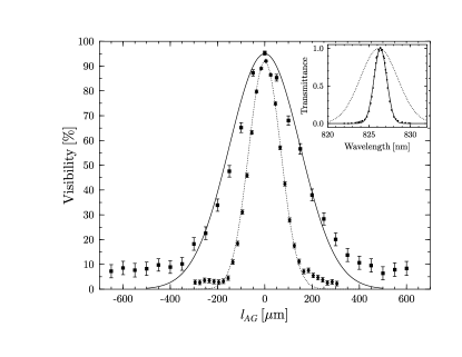
Figure 2: Coincidence-count interference visibility between detectors D_2A and D₁ as a function of the air-gap position. Diamonds correspond to the measurement without any filter. The dotted curve is a Gaussian fit according to Eq. (12) yielding the geometric spectral filtering of FWHM=5.3 nm. The spectrum calculated according to Eq. (9) is plotted with the dotted curve in the inset. Squares correspond to the measurement with the narrow band interference filter. The continuous curve is the theoretical dependence obtained for the parameters of the filter provided by the manufacturer. The inset shows the normalized transmittance of the filter (dots) and a Gaussian fit of these data (continuous curve) yielding a FWHM of 1.8 nm.

First we use the setup shown in Fig. 1 without the FP resonator. Figure 2 shows the visibility of interference pattern in the measured coincidence-count rate between detectors D_2A and D₁ as a function of the air-gap position. The visibility reaches significant values only in a region whose width is inversely proportional to the bandwidths of the signal and idler spectra (see Eq. (12)). Diamonds correspond to the measurement without any filter, thus showing the effect of the geometric filtering of the fiber-coupling optics. Plotted errors represent the standard deviations. The dotted curve is a Gaussian fit of these data with a FWHM of 160 $\mu$m, which corresponds to a spectrum of 5.3 nm FWHM. This spectrum of the signal photons, calculated according to Eq. (9), is plotted with the dotted curve in the inset of Fig. 2.

Squares in Fig. 2 correspond to the coincidence-count interference visibility measured in the setup modified by inserting the narrow band interference filter centered at 826.4 nm (Andover Corporation) in the signal-beam path. Dots in the inset show the measured normalized transmittance of the filter provided by the manufacturer, and the continuous curve is a Gaussian fit of these experimental data with a FWHM of 1.8 nm. The parameters of the filter yield theoretical visibility dependence of a 350 $\mu$m FWHM (continuous curve). This curve fits well the experimental data (squares) in the central part of the pattern. The deviations from the Gaussian shape in the low-visibility wings are caused by the difference of the real spectrum of the filters from the Gaussian shape, as can be shown by a more detailed analysis tractable only numerically. The narrowing of the spectrum of signal photons from 5.3 nm to 1.8 nm thus leads to the broadening of the coincidence-count interference pattern from 160 $\mu$m to 350 $\mu$m.

Figure 3: Coincidence-count interference visibility between detectors D_2A and D₁ as a function of the air-gap position $l_{AG}$. Squares correspond to the measurement setup with the FP resonator in the signal-photon path. Curves are the fits given according to Eq. (15) with the parameter $F=150$. The dotted curve: $l_{F}$=95.00 $\mu$m, the continuous curve: $l_{F}$=94.86 $\mu$m, the dashed curve: $l_{F}$=94.80 $\mu$m.

Figure 3 shows the coincidence-count interference visibility measured with the FP resonator. The length of the resonator $l_{F}$ can be tuned over a range of 1.5 $\mu$m. The high-visibility region is now considerably wider than the one obtained in the previous case, but we get a modulated curve described by Eq. (15) instead of a single-peak function. The period of the measured visibility oscillations is given by one roundtrip in the FP resonator 2$l_{F}$, yielding the resonator length $l_{F}\approx 95~{}\mu$m. We note that similar oscillations in interference patterns were observed in Gisin , where properties of entangled photon pairs generated by a train of pump pulses were studied.

The free spectral range of the FP resonator expressed in units of wavelength is $\lambda_{FSR}=\frac{1}{2}\lambda^{2}/l_{F}\approx 3.6$ nm. Compared to the 5.3 nm FWHM of the geometric spectrum of signal photons, it is obvious that more than one peak of the FP contributes to the signal at detector D₁. If we change the FP length $l_{F}$ by one quarter of the wavelength, the modulation of visibility changes from one limiting case to another according to the changes of the spectrum of the transmitted signal photons. $l_{F}=95.00~{}\mu$m corresponds to the first limiting case. The theoretical spectrum has one dominant peak at the center and two weak satellites; the visibility modulation is smallest (dotted curve in Fig. 3). For $l_{F}=94.80~{}\mu$m, the visibility modulation is largest, corresponding to the second limiting case (dashed curve in Fig. 3). In this case the spectrum is composed of two dominant equivalently strong maxima. The other two small maxima prevent the visibility from reaching zero at its minima. Comparing the theory with the experimental data, we have found that the FP resonator length that provides the measured visibility modulation is $l_{F}=94.86\mu$m (solid line in Fig. 3). The spectrum corresponding to this FP length is shown in Fig. 4.

Figure 4: The continuous curve is the spectrum of the signal photons calculated according to Eq. (13) that yields the measured visibility modulation of Fig. 3 ($l_{F}$=94.86 $\mu$m). The dotted curve represents the geometric filtering (FWHM=5.3 nm).

Figure 5: Coincidence-count interference visibility between detectors D_2A and D₁ as a function of the air-gap position. Diamonds correspond to the measurement setup without any filter. The dotted curve is a Gaussian fit given by Eq. (12), corresponding to spectral FWHM=5.3 nm. Squares correspond to the measurement setup with both the FP resonator and the narrow band interference filter in the signal-photon path. The continuous curve is the fit according to Eq. (15) with parameters $F=150$ and $l_{F}$=95.03 $\mu$m. The inset shows the calculated spectra of the signal photons, Eq. (13). The dotted curve corresponds to the geometric filtering (FWHM=5.3 nm), the continuous curve represents the transmittance of the FP resonator together with the narrow band filter.

To avoid the effect of multiple frequency peaks transmitted through the FP resonator, we use a combination of both filters (the FP resonator and the narrow band interference filter) in the signal-photon path. Figure 5 shows both the measured coincidence-count interference visibility (squares) and the theoretical curve (continuous curve) according to Eq. (15). For comparison, the dependences obtained for the setup with no filter are plotted as well (diamonds and dotted curve, same as in Fig. 2). Using both filters in the signal-photon path we are able to select just one narrow transmittance peak of the FP resonator. This is possible because the narrow band filter’s FWHM is smaller than the FP’s free spectral range. Scanning the FP’s length we are able to position this narrow transmittance peak to the center of the interference filter, $l_{F}$=95.03 $\mu$m, see the continuous line in the inset in Fig. 5. With this setting there are no oscillations in the visibility pattern any more.

From Fig. 5 we can clearly see that while there is no interference in the MZ interferometer detuned from the balanced position by a few millimeters in the idler beam, a high visibility can be achieved in coincidence-count measurements by placing a narrow frequency filter in the path of signal photons. This is a direct consequence of the strong energy correlations between the two entangled beams. One can also see this experiment from another point of view: The FP resonator serves as a postselection device that selects a quasi-monochromatic component of the signal beam. This selection is done in the idler beam by means of the coincidence-count measurement, thus yielding a wide autocorrelation function of the postselected idler beam.

V Time correlations

First we describe theoretical results obtained for the Hong-Ou-Mandel interferometer. The coincidence-count rate $R_{n}^{HOM}$ as a function of relative delay $\Delta t$ between the signal and idler photons is determined in terms of the two-photon amplitude ${A}$ given in Eq. (3) as follows Perina_PRA59

$$R_{n}^{HOM}(\Delta t)=1-\rho^{HOM}(\Delta t),\mbox{where}$$

$$\rho^{HOM}(\Delta t)=\frac{\int_{-\infty}^{\infty}dt_{A}\int_{-\infty}^{\infty}dt_{B}{\rm Re}\left\{{A}(t_{A}-\Delta t,t_{B}){A}^{*}(t_{B}-\Delta t,t_{A})\right\}}{\int_{-\infty}^{\infty}dt_{A}\int_{-\infty}^{\infty}dt_{B}\left|{A}(t_{A},t_{B})\right|^{2}}.$$ (18)

Assuming that the spectrum of signal and idler photons is determined by the geometric filtering according to Eq. (9) with parameters $\sigma_{1}=\sigma_{2}=\sigma$, the interference term $\rho^{HOM}$ of Eq. (18) assumes the form

$$\rho^{HOM}(\Delta t)=\exp\left[-\frac{\sigma^{2}\Delta t^{2}}{2}\right].$$ (19)

The width of the dip given by $\rho^{HOM}$ is half the width of the visibility peak given by Eq. (12) in the case of geometric filtering without any additional filters.

Figure 6: Experimental setup for the Hong-Ou-Mandel interference measurement. The photon-pair source (NLC) and the fiber-coupling optics are identical to that shown in Fig. 1. FC is a fiber coupler, D₁ and D₂ are photodetectors, C denotes detection electronics.

Figure 7: Coincidence-count interference pattern in the Hong-Ou-Mandel interferometer as a function of the path difference of the interferometer’s arms. The continuous curve is a Gaussian fit given by Eq. (19). The FWHM of the coincidence-count dip is 72 $\mu$m.

It is necessary to emphasize that the experiment as performed in the previous section is not a proof of the strong quantum correlations produced by the entangled state of Eq. (1). For instance, if the source emitted two monochromatic photons with classically correlated frequencies $\omega_{1}$ and $\omega_{2}$ (in the sense of a statistical ensemble) with a proper classical probability density $p(\omega_{1},\omega_{2})$, the same increase of visibility in the coincidence-count measurement with a FP resonator and a MZ interferometer would be obtained Dusek_CJP46 . However, such a source could never give the tight time correlations of detection instants observed in the HOM interferometric setup Hong_PRL59 . In order to confirm the validity of the description based on the entangled two-photon state, we performed a time correlation measurement in the HOM interferometer with our source of photon pairs.

Figure. 6 shows a scheme of the HOM interferometric setup. The time difference $\Delta t$ is obtained by translating the fiber-coupling collimator in one of the HOM interferometer’s arms towards the nonlinear crystal. The width of the measured coincidence-count dip (see Fig. 7) is 72 $\mu$m which yields the coherence time of the down-converted photons of 240 fs and the spectral FWHM of 6.0 nm. This spectral width is slightly larger than the one obtained with the MZ interferometer (5.3 nm). The difference of these two results is due to a slight readjustment needed after changing the experimental setup (compare Figs. 6 and 1).

VI Conclusions

Second- and fourth-order interference experiments testing the nature of entangled two-photon fields generated in spontaneous parametric down-conversion have been studied. Energy correlations were observed by frequency filtering of signal photons, while the idler photons propagated through a Mach-Zehnder interferometer. It has been demonstrated that even if the MZ interferometer is unbalanced to the extent that no interference can be observed, interference with a high visibility is restored in the coincidence-count detections provided that the signal photons are transmitted through a narrow frequency filter. Theoretical results obtained in the presented model for a Gaussian filter, Fabry-Perot resonator or both filters together are in good agreement with our experimental results. Tight time correlations have been observed in the Hong-Ou-Mandel interferometer.

It should be stressed that both experiments inspecting energy correlations and time correlations provide complementary information about the generated photon state. The same results in each individual experiment can be obtained with classical fields, but there is no classical model that could explain both of them together. This shows that the two-photon state generated in the process of spontaneous parametric down-conversion is properly described by the entangled two-photon state of Eq. (1), because it is this entangled two-photon state that can explain both energy and time correlations together.

VII ACKNOWLEDGEMENTS

This research was supported by the Ministry of Education of the Czech Republic under grants LN00A015, CEZ J14/98, RN19982003012, and by EU grant under QIPC project IST-1999-13071 (QUICOV). The authors would like to thank A. Lukš and V. Peřinová for help with mathematical derivations.

References

- (1) C.K. Hong, L. Mandel, Phys. Rev. A 31, 2409 (1985).
- (2) J. Peřina, Z. Hradil, and B. Jurčo: Quantum Optics and Fundamentals of Physics (Kluwer, Dordrecht, 1994).
- (3) M.H. Rubin, Phys. Rev. A 54, 5349 (1996).
- (4) T.B. Pittman, Y.H. Shih, D.V. Strekalov, A.V. Sergienko, Phys. Rev. A 52, R3429 (1995).
- (5) T.B. Pittman, D.V. Strekalov, D.N. Klyshko, M.H. Rubin, A.V. Sergienko, Y.H. Shih, Phys. Rev. A 53, 2804 (1996).
- (6) C.H. Monken, P.H.S. Ribeiro, S. Pádua, Phys. Rev. A 57, 3123 (1998).
- (7) C.K. Hong, Z.Y. Ou, L. Mandel, Phys. Rev. Lett. 59, 2044 (1987).
- (8) T.B. Pittman, D.V. Strekalov, A. Migdall, M.H. Rubin, A.V. Sergienko, Y.H. Shih, Phys. Rev. Lett. 77, 1917 (1996).
- (9) P.G. Kwiat, A.M. Steinberg, R.Y. Chiao, Phys. Rev. A 45, 7729 (1992).
- (10) Z.Y. Ou, L. Mandel, Phys. Rev. Lett. 61, 50 (1988).
- (11) J.D. Franson, Phys. Rev. Lett. 62, 2205 (1989).
- (12) J. Brendel, E. Mohler, W. Martienssen, Phys. Rev. Lett. 66, 1142 (1991).
- (13) J.G. Rarity, P.R. Tapster, Phys. Rev. A 45, 2052 (1992).
- (14) P.G. Kwiat, A.M. Steinberg, R.Y. Chiao, Phys. Rev. A 47, R2472 (1993).
- (15) X.Y. Zou, T.P. Grayson, L. Mandel, Phys. Rev. Lett. 69, 3041 (1992).
- (16) T. Tsegaye, G. Björk, M. Atatüre, A.V. Sergienko, B.E.A. Saleh, M.C. Teich, Phys. Rev. A 62, 032106 (2000).
- (17) P.G. Kwiat, R. Y. Chiao, Phys. Rev. Lett. 66, 588 (1991).
- (18) M. Dušek, Czech. J. Phys. 46, 921 (1996).
- (19) P. Trojek, J. Peřina, Jr., Czech. J. Phys. 53, 335 (2003).
- (20) J.D. Franson, Phys. Rev. Lett. 67, 290 (1991).
- (21) Z.Y. Ou, L.J. Wang, L. Mandel, Phys. Rev. A 40, 1428 (1989).
- (22) W.P. Grice, I.A. Walmsley, Phys. Rev. A 56, 1627 (1997).
- (23) J. Peřina Jr., A.V. Sergienko, B.M. Jost, B.E.A. Saleh, M.C. Teich, Phys. Rev. A 59 2359 (1999).
- (24) J. Peřina Jr., Eur. Phys. J. D 7 235 (1999).
- (25) M. Atatüre, G. Di Giuseppe, M.D. Shaw, A.V. Sergienko, B.E.A. Saleh, M.C. Teich, Phys. Rev. A 66, 023822 (2002).
- (26) Y. Nambu, K. Usami, Y. Tsuda, K. Matsumoto, K. Nakamura, Phys. Rev. A 66, 033816 (2002).
- (27) B.E.A. Saleh, M.C. Teich: Fundamentals of Photonics (J. Wiley, New York, 1991).
- (28) J. Peřina. Jr., Characterization of a resonator using entangled two-photon states, to be published.
- (29) H. de Riedmatter, I. Marcikic, H. Zbynden, M. Gisin, Quant. Inf. and Cumputation 2, 425 (2002).