Decoherence without dissipation?

Abstract

In a recent article,Ford et al. (2001) Ford, Lewis and O’Connell discuss a thought experiment in which a Brownian particle is subjected to a double-slit measurement. Analyzing the decay of the emerging interference pattern, they derive a decoherence rate that is much faster than previous results and even persists in the limit of vanishing dissipation. This result is based on the definition of a certain attenuation factor, which they analyze for short times. In this note, we point out that this attenuation factor captures the physics of decoherence only for times larger than a certain time $t_{\mathrm{mix}}$, which is the time it takes until the two emerging wave packets begin to overlap. Therefore, the strategy of Ford et al of extracting the decoherence time from the regime $t<t_{\mathrm{mix}}$ is in our opinion not meaningful. If one analyzes the attenuation factor for $t>t_{\mathrm{mix}}$, one recovers familiar behaviour for the decoherence time; in particular, no decoherence is seen in the absence of dissipation. The latter conclusion is confirmed with a simple calculation of the off-diagonal elements of the reduced density matrix.

I Introduction

It is widely accepted that a rapid loss of coherence caused by the coupling to environmental degrees of freedom is at the root of the non-observation of superpositions of macroscopically distinct quantum states. There is a now well established theoretical scheme—“Dissipative Quantum Mechanics”—for studying the details of this phenomenon, and for analyzing its time scale.see e.g. U. Weiss (1993) It has also become possible to observe decoherence in a variety of experiments in mesoscopic physics Chiorescu et al. (2003); Nakamura et al. (1999) and quantum optics. Kokorowski et al. (2001); Arndt et al. (1999)

In a recent publication,Ford et al. (2001) Ford, Lewis and O’Connell (henceforth abbreviated as FLO) discuss a thought experiment in which a Brownian particle initially in thermal equilibrium with its environment is subjected to a double-slit position measurement, giving rise to an interference pattern. Analyzing the decay of this pattern, they derive a decoherence time that is much shorter than suggested by previous calculation.see e.g. A. Venugopalan (1999) They suggest the tentative explanation that inital particle-bath correlations, which drastically alter the short-time behaviour of the Brownian particle, were not properly taken into account in previous work. Because the decoherence time calculated by FLO remains finite even in the absence of any coupling to the environment, they describe their result as decoherence without dissipation.Ford and O’Connell (2001)

This is very puzzling. The usual physical picture of decoherencesee e.g. U. Weiss (1993); Amvegaokar (1993) is that averaging over unobserved degrees of freedom (the “environment”) leads to non-unitary time evolution, with a consequent loss of information. If there is no coupling to the environment, there will be no such loss. This picture agrees with another commonly accepted definition of decoherence, as the decay of the off-diagonal elements of the reduced density matrix (more precisely, the decay of the interference part $\rho_{\mathrm{int}}$ to be defined in section VI). Without environmental coupling, the time evolution of the system – and thus of $\rho_{\mathrm{int}}$ – is unitary, the norm of $\rho_{\mathrm{int}}$ is constant and does not decay.

In light of these obvious remarks, it is interesting to ask what FLO mean by decoherence. In this type of double slit experiment it is essential that the two initially separated parts of the wave function eventually overlap if an interference pattern in the probability density of the particle is to be observed.Caldeira and Leggett (1985) In the thought experiment considered by FLO, this overlap becomes sizeable only after the broadening of the two wave packets emerging from either slit becomes equal to their initial separation, which happens after a certain timescale $t_{\mathrm{mix}}$, to be defined in Eq. (11) below. On much shorter time scales, the interference pattern is not only influenced by the presence (or absence) of coherence, but also by the degree of overlap of the wave functions, which makes it difficult, if not impossible, to extract from the probability density alone a quantitative measure of decoherence that is meaningful for $t<t_{\mathrm{mix}}$. As will be shown, the decoherence time obtained by FLO is much shorter than $t_{\mathrm{mix}}$ and hence merely reflects an arbitrariness in the definition of decoherence at these short time scales.

The outline of this paper is as follows: In the following section, we give a brief summary of FLO’s work and present, in section III, the results of an alternative derivation (given in appendix A) of the probability density of the particle, which fully agrees with that of FLO. Section IV demonstrates that dynamic effects (i.e. the spreading of the wave packets), rather than actual decoherence effects, enter FLO’s definition of decoherence for times shorter than $t_{\mathrm{mix}}$. This fact is further illustrated in section V in which a definition of decoherence is given that incorporates the wave packet spreading in a different (and equally arbitrary) way, but gives rise to an entirely different picture on these short time scales. Finally, in section VI, the off-diagonal elements of the reduced density matrix, which allow the definition of a decoherence measure valid also for $t<t_{\mathrm{mix}}$, are analyzed, and no decoherence without dissipation is found.

II Summary of Ford, Lewis and O’Connell’s results

In the thought experiment discussed by FLO,Ford et al. (2001) a one-dimensional free Brownian particle, in thermal equilibrium with its environment, is suddenly (at time $t_{1}=0$, say) subjected to a double-slit position measurement. This measurement is described as a weighted sum of projectors $P=\int dx\alpha(x)|x\rangle\langle x|$ acting from the left and right on the density matrix, such that after the measurement, the state is described as

$$\rho_{\mathrm{ini}}(x,x^{\prime},\{Q_{\alpha}\},\{Q_{\alpha}^{\prime}\})$$ (1)

$$= \alpha^{*}(x)\alpha(x^{\prime})\rho_{\mathrm{th}}(x,x^{\prime},\{Q_{\alpha}\},\{Q_{\alpha}^{\prime}\}),$$

where $\rho_{\mathrm{th}}(x,x^{\prime},\{Q_{\alpha}\},\{Q_{\alpha}^{\prime}\})$ denotes the density matrix of a particle (described by the coordinate $x$) in thermal equilibrium with its environment (described by a set of coordinates $Q_{\alpha}$). The measurement function $\alpha$ describes the transmittance of the double slit and is taken as a sum of two Gaussian functions with width $2\sigma$, and separated by a distance $d\gg\sigma$:

$$\alpha(x)=\frac{N^{1/2}}{(8\pi\sigma^{2})^{1/4}}\cdot\left(e^{-\frac{(x-d/2)^{2}}{4\sigma^{2}}}+e^{-\frac{(x+d/2)^{2}}{4\sigma^{2}}}\right),$$ (2)

$N=(1+e^{-d^{2}/(8\sigma^{2})})^{-1}$ being a normalization constant, such that $\int dx|\alpha(x)|^{2}=1$. The particle dynamics are calculated in the framework of a quantum Langevin equation,Ford and Kac (1987); Ford and Lewis (1986) which describes the dynamics of a particle coupled to a dissipative environment with Ohmic characteristics.

Within this framework, FLO calculate the probability density $P(x,t)=\tilde{\rho}(x,x,t)$ for finding the particle at time $t$ at coordinate $x$, $\tilde{\rho}$ being the reduced density matrix of the Brownian particle. Because the initial state $\rho_{\mathrm{ini}}$ describes a superposition of the particle emanating from either slit, $P(x,t)$ displays a spatial interferece pattern, from which FLO extract an attenuation factor $a_{\mathrm{FLO}}(t)$. The decay of $a_{\mathrm{FLO}}(t)$ allows them to define the decoherence time $\tau^{D}_{\mathrm{FLO}}$ discussed in the previous section and below.

III Derivation of $P(x,t)$

Because the reader may not be familiar with the framework of the quantum Langevin equation, we include a different derivation of $P(x,t)$ in a path integral framework in Appendix A. The result is

$$P(x,t)=P_{\mathrm{cl}}(x,t)+P_{\mathrm{int}}(x,t)\cos\left(\frac{xdA(t)}{2\sigma^{2}w(t)^{2}}\right),$$ (3)

with

$$P_{\mathrm{cl}}(x,t) = \frac{N}{2}\left(P_{1}(x-d/2,t)+P_{1}(x+d/2,t)\right)$$ (4)

$$\equiv \frac{1}{2}\left(P_{\mathrm{cl}}^{-}(x,t)+P_{\mathrm{cl}}^{+}(x,t)\right),$$

$$P_{1}(x,t)=\frac{1}{\sqrt{2\pi w(t)^{2}}}\cdot\exp\left(-\frac{x^{2}}{2w(t)^{2}}\right),$$ (5)

$$P_{\mathrm{int}}=\frac{N}{\sqrt{2\pi w(t)^{2}}}\cdot\exp\left(-\frac{x^{2}+d^{2}(\sigma^{2}-2Q(t))/(4\sigma^{2})}{2w(t)^{2}}\right),$$ (6)

the width $w(t)$ of the wave packets being

$$w(t)^{2}=\sigma^{2}+\frac{A(t)^{2}}{\sigma^{2}}-2Q(t).$$ (7)

The quantities $A(t)$ and $Q(t)$ are defined as the imaginary and real part of the position-position autocorrelation function $\langle(x(t)-x(0))x(0)\rangle\equiv Q(t)+iA(t)$, and are related to the parameters in FLO’s work by

$$[x(t_{1}),x(t_{1}+t)]=2iA(t),\;\;\;s(t)=-2Q(t).$$ (8)

As is shown in Appendix A, $P_{1}(x\mp d/2,t)$ is the probability distribution if only one slit, centered around $x=\pm d/2$, was present; $P_{\mathrm{int}}(x,t)$ is the amplitude of the interference pattern. The resulting expression (3) for $P(x,t)$ agrees with FLO’s result.

The explicit form of $A(t)$ and $Q(t)$ in the case of an Ohmic heat bath with infinite cutoff and friction coefficient $\gamma$ is quite cumbersome and given in Eq. (9.14) and (9.15) of [Grabert et al., 1988]. However, for our purposes the limiting case $\gamma\ll T$ will be sufficient, which we assume from now on. In this case, $A(t)$ and $Q(t)$ are given by

$$A(t)=\frac{1-e^{-\gamma t}}{2m\gamma},\;\;Q(t)=-\frac{T}{m\gamma}\left(t-\frac{1-e^{-\gamma t}}{\gamma}\right).$$ (9)

For $\gamma=0$, these equations reduce to

$$A(t)=\frac{t}{2m},\;\;Q(t)=-\frac{Tt^{2}}{2m}$$ (10)

Above and hereafter, we chose units with $\hbar=k_{B}=1$. After the mass, length and energy scales are set by the particle mass $m$, the distance of the slits $d$, and by $E\equiv m^{-1}d^{-2}$, there are three remaining free parameters in the theory: the slit width $\sigma/d$, the temperature $T/E$, and the friction coefficient of the Ohmic heat bath $\gamma/E$. In all plots below, we set the slit width as $\sigma=d/20$ unless otherwise stated.

IV Critique of FLO’s analysis

Before we comment on the further analysis of FLO, we shall briefly discuss some properties of the probability density $P(x,t)$.

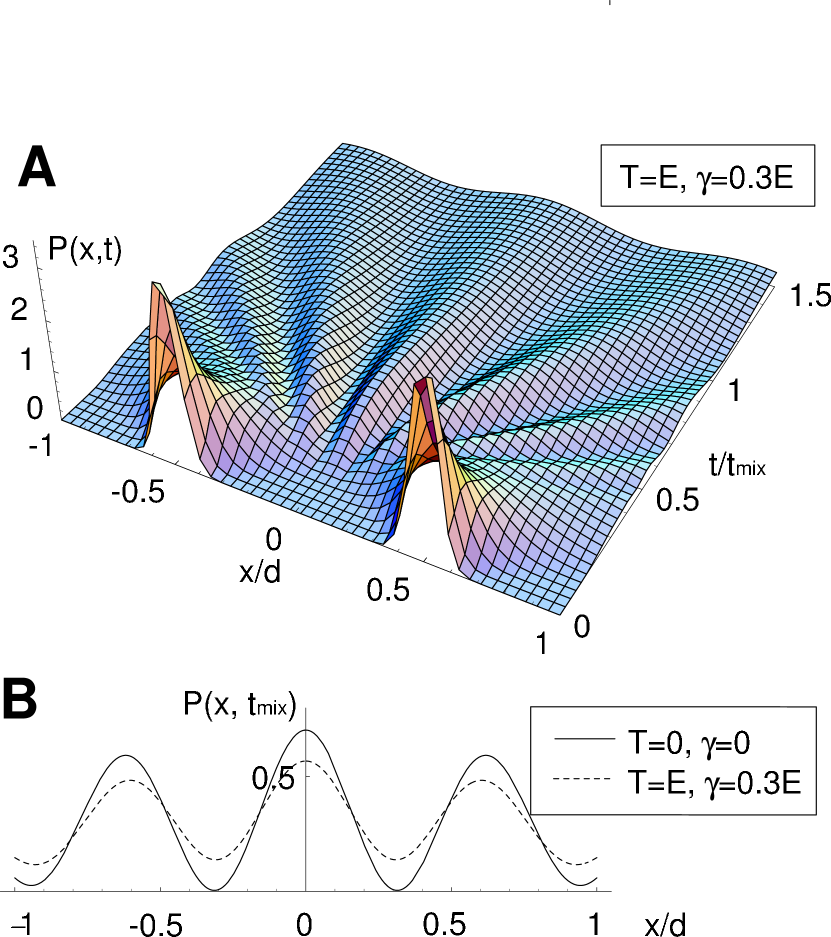
Figure 1: A: The probability density $P(x,t)$ for finding the particle at time $t$ at coordinate $x$ is plotted for $T=E,\gamma=0.3E$. An interference fringe is seen to appear at time $t_{\mathrm{mix}}$. B: $P(x,t=t_{\mathrm{mix}})$ is plotted for the same parameters as in A (dashed line), and for $T=\gamma=0E$ (solid line). The interference fringe in the former curve is seen to be somewhat suppressed with respect to the latter, but to be qualitatively very similar.

In Fig. 1A, $P(x,t)$ is plotted for the parameters $\gamma=0.3E$, $T=E$ (in the following, these parameters will be referred to as the weak dissipation case). An interference pattern is seen to emerge only after the two wave packets, initially separated by $d$, have developed a significant overlap. The associated time scale $t_{\mathrm{mix}}$ is implicitly given by $w(t_{\mathrm{mix}})=d$. As long as friction and thermal spreading of the wave packets is dominated by quantum broadening ($\gamma\ll T\ll E\cdot d^{2}/\sigma^{2}$), $t_{\mathrm{mix}}$ is given by

$$t_{\mathrm{mix}}\equiv 2m\sigma d,$$ (11)

which we will use as a definition of $t_{\mathrm{mix}}$ from now on. For $t<t_{\mathrm{mix}}$, the interference pattern is influenced not only by the loss of phase coherence, but also (and mainly) by the spreading of the wave packets, as is shown below. For $t>t_{\mathrm{mix}}$, the interference pattern is seen to broaden and to become flatter, as the wave function continues to spread.

In Fig. 1B, the interference pattern at time $t=t_{\mathrm{mix}}$ in the weak dissipation case is compared to the case $T=\gamma=0$. In Fig. 2, $P(x,t)$ is shown for three different times, again using the parameters of the weak dissipation case, together with the noninterfering part of the amplitude $P_{\mathrm{cl}}(x,t)$ and with the envelope of the interference pattern, given by $P_{\mathrm{cl}}(x,t)\pm P_{\mathrm{int}}(x,t)$.

Figure 2: $P(x,t)$ is shown at the times $t=0.1\cdot t_{\mathrm{mix}}$; $t=0.3\cdot t_{\mathrm{mix}}$; and $t=t_{\mathrm{mix}}$ (from top to bottom), for the parameters $T=E$, $\gamma=0.3E$ (thick line). Also shown: The noninterfering contribution $P_{\mathrm{cl}}(x,t)$ (thin line) and the envelope $P_{\mathrm{cl}}(x,t)\pm P_{\mathrm{int}}(x,t)$ of the interference pattern (dashed line) around $P_{\mathrm{cl}}(x,t)$.

As can be seen in Fig. 2, $P_{\mathrm{cl}}(x=0,t)$ is vanishingly small at $t\ll t_{\mathrm{mix}}$, and is rapidly growing as the wave packets start to overlap. When the temperature is further increased, $P_{\mathrm{cl}}(x=0,t)$ grows even faster for $t<t_{\mathrm{mix}}$ due to the additional thermal spreading of the wave packets (not shown).

In Fig. 1B, the interference fringes for the case of no dissipation on the one hand and for weak dissipation on the other hand look quite similar. This is in drastic contrast to what one might expect from FLO’s analysis, which leads to a decoherence time given by

$$\tau^{D}_{\mathrm{FLO}}=\frac{s^{2}m^{1/2}}{dT^{1/2}}.$$ (12)

The parameters chosen for the weak dissipation case in Fig. 1B imply, for example, $\tau^{D}_{\mathrm{FLO}}=0.025\cdot t_{\mathrm{mix}}$ (extracted from the very same function $P(x,t)$!). We believe this value implies that by the time $t_{\mathrm{mix}}$, the entire interference pattern, clearly visible in Fig. 1, should have already disappeared. How can this be?

The decoherence analysis of FLO is based on an attenuation factor $a_{\mathrm{FLO}}(t)$, which is defined as “the ratio […] of the amplitude of the interference term to twice the geometric mean of the other two terms” Ford et al. (2001), i.e. as

$$a_{\mathrm{FLO}}(t)=\frac{P_{\mathrm{int}}(x,t)}{\sqrt{P_{\mathrm{cl}}^{+}(x,t)\cdot P_{\mathrm{cl}}^{-}(x,t)}}.$$ (13a)

An example of $$a_{\mathrm{FLO}}(t) a_{\mathrm{FLO}}(t)$$ is shown in Fig. 3 (dashed line). Using Eqs. (4) to (6), can be recast in the form

$$a_{\mathrm{FLO}}(t)=\frac{P_{\mathrm{int}}(x=0,t)}{P_{\mathrm{cl}}(x=0,t)}.$$ (13b)

In other words, $a_{\mathrm{FLO}}$ measures the interference amplitude $P_{\mathrm{int}}$ in units of the classical amplitude $P_{\mathrm{cl}}$ at $x=0$; hence it does not merely measure the time dependence of the interference pattern, but also reflects the drastic increase of the reference unit $P_{\mathrm{cl}}(x=0,t)$ for $t<t_{\mathrm{mix}}$.

Figure 3: $P_{\mathrm{cl}}(x=0,t)$ and $P_{\mathrm{int}}(x=0,t)$ (dotted and solid line) are shown along with their ratio $a_{\mathrm{FLO}}=P_{\mathrm{int}}/P_{\mathrm{cl}}$ (dashed line) for $T=E$, $\gamma=0$. Both $P_{\mathrm{int}}$ and $P_{\mathrm{cl}}$ grow rapidly after time $t_{\mathrm{spread}}$, after which thermal broadening of the wave packets begins. $a_{\mathrm{FLO}}$ is seen to drop only for $t<t_{\mathrm{spread}}$.

This is illustrated in Fig. 3, where $P_{\mathrm{int}}(x=0,t)$ and $P_{\mathrm{cl}}(x=0,t)$ are plotted along with their ratio $a_{\mathrm{FLO}}(t)$ for finite temperature $T=E$ and no dissipation ($\gamma=0$). Using Eq. (5), (6), the exponents in $P_{\mathrm{int}}$ and $P_{\mathrm{cl}}$ are seen to be only slowly departing from their initial values $P_{\mathrm{int}}(t=0),P_{\mathrm{cl}}(t=0)\sim\exp(-d^{2}/8\sigma^{2})$ ($\sim 10^{-22}$ for the given parameters!) as long as $t<t_{\mathrm{spread}}\equiv t_{\mathrm{mix}}\;\sigma/d$. This is because for $t<t_{\mathrm{spread}}$ the wave packet width $w(t)$ in Eq. (7) is dominated by the constant $\sigma^{2}$, and that quantum spreading is not effective yet. The rapid growth of $P_{\mathrm{int}}(t)$ and $P_{\mathrm{cl}}(t)$ by 22 orders of magnitude seen in Fig. 3 takes place almost entirely between $t_{\mathrm{spread}}$ and $t_{\mathrm{mix}}$, when the overlap of the wave packets increases rapidly due to quantum spreading. On the other hand, the decrease of $a_{\mathrm{FLO}}$ takes place before $t_{\mathrm{spread}}$, when $P_{\mathrm{int}}$ and $P_{\mathrm{cl}}$ are still tiny. Indeed, $t<t_{\mathrm{spread}}$ is precisely the condition that $a_{\mathrm{FLO}}$ can be fitted by a Gaussian, $a_{\mathrm{FLO}}\approx\exp(-t^{2}/8(\tau^{D}_{\mathrm{FLO}})^{2})$, from which $\tau^{D}_{\mathrm{FLO}}$ was extracted by FLO. Once quantum broadening sets in after $t_{\mathrm{spread}}$, $a_{\mathrm{FLO}}$ crosses over to a constant.

In summary, $a_{\mathrm{FLO}}$ is seen to reflect mainly the details of the broadening of the wave packets, and therefore does not appear to us to be a suitable measure for their coherence.

V Alternative analysis of $P(x,t)$

As long as the overlap of the two wave packets is held fixed, the amplitude of the interference pattern $P_{\mathrm{int}}(x,t)$ is, indeed, a direct measure of their phase coherence. Similar interference patterns have been analyzed to this purpose in a number of very illuminating experiments, most explicitly in [Kokorowski et al., 2001]. In the thought experiment considered here, the wave packets overlap only after a time $t_{\mathrm{mix}}$. This introduces a considerable amount of arbitrariness in a definition of decoherence for times $t<t_{\mathrm{mix}}$, if this definition is based upon the diagonal elements of the reduced density matrix $P(x,t)=\tilde{\rho}(x,x,t)$ only. For the regime $t<t_{\mathrm{mix}}$, an unambiguous measure of decoherence can only be obtained from the decay of the off-diagonal elements of the reduced density matrix $\tilde{\rho}$, as for example in [Strunz and Haake, 2003]. However, this would go beyond the scope of the present article, and such an analysis is only done for the dissipationless case $\gamma=0$ (in section VI). In this section, we take a less ambitious approach and just give an example showing how, for these short times, a different definition of an attenuation factor based on the probability density (i.e. the diagonal elements of $\tilde{\rho}$) results in a picture completely different from that of FLO.

For this purpose, we introduce the attenuation factor

$$a_{2}(t)=\frac{P_{\mathrm{int}}(x=0,t)}{N\cdot P_{1}(x=0,t)},$$ (14)

where $P_{1}$ and $P_{\mathrm{int}}$ are defined in Eq. (5) and Eq. (6), and $N$ is the trivial normalization factor defined after Eq. (2). Similarly to $a_{\mathrm{FLO}}$, this measures the relative importance of the interference amplitude $P_{\mathrm{int}}$ with respect to the noninterfering contribution. The difference with respect to $a_{\mathrm{FLO}}(t)$ in Eq. (13b) is that the relative importance of the noninterfering part of $P(x,t)$ is captured in a slightly different (but by no means less arbitrary) way. In order to make the connection to the quantities shown in Fig. 2, $N\cdot P_{1}(x=0,t)$ is proportional to the heigth of $P_{\mathrm{cl}}$ at the center of one of the slits (i.e.  at $x=\pm 0.5d$), whereas in the definition of $a_{\mathrm{FLO}}$ the value at $x=0$ was taken as reference unit.

We would like to emphasize that our $a_{2}$ is not “better” or “more appropriate” than $a_{\mathrm{FLO}}$. Indeed, for $t>t_{\mathrm{mix}}$, $a_{2}$ and $a_{\mathrm{FLO}}$, and hence all conclusions drawn from them, are the same. For short times $t<t_{\mathrm{mix}}$, however, $a_{\mathrm{FLO}}$ and $a_{2}$ differ wildly; this illustrates that on these short time scales, both definitions are dominiated by effects of wave packet spreading rather than decoherence, albeit in a different way. We would like to emphasize that the condition $a_{\mathrm{FLO}}(t=0)=1$ that distinguishes $a_{\mathrm{FLO}}$ from $a_{2}$ is in our opinion not necessary, because at times $t\ll t_{\mathrm{mix}}$, the attenuation factors have nothing to say about decoherence anyway.

Figure 4: The attenuation factors $a_{2}(t)$ from Eq. (14) (solid line) and $a_{\mathrm{FLO}}(t)$ from Eq. (13b) (dashed line) are compared and seen to be wildly different for $t<t_{\mathrm{mix}}$. $a_{2}$ is related to $P_{\mathrm{int}}$ in Fig. 3, the only difference being that the prefactor $(2\pi w^{2})^{-1/2}$ present in Eq. (6) for $P_{\mathrm{int}}$ is missing in $a_{2}$. Inset: The attenuation factor $a_{2}(t)$ is plotted as a function of time, for $T=\gamma=0$, for $T=E$, $\gamma=0$, and for $T=E$, $\gamma=0.3E$ (from top to bottom).

In Fig. 4, the time evolution of $a_{2}$ and $a_{\mathrm{FLO}}$ are compared for finite temperature $T=E$ and $\gamma=0$. $a_{\mathrm{FLO}}$ is seen to decay from the initial value $a_{\mathrm{FLO}}(t=0)=1$, whereas $a_{2}$ is growing, more closely resembling the actual interference pattern seen in Fig. 1. For $t>t_{\mathrm{mix}}$, both $a_{\mathrm{FLO}}$ and $a_{2}$ become equal and saturate at the value

$$a^{\infty}=\exp\left(-\frac{d^{2}}{8\sigma^{2}+2\lambda_{\mathrm{th}}^{2}}\right),$$ (15)

where $\lambda_{\mathrm{th}}^{2}=1/(mT)$ is the squared thermal wavelength. As is shown in section VI below, the reduction of $a^{\infty}$ at finite temperature results from the imperfect preparation of the initial state, and has no time scale associated with it, contrary to what the time evolution of $a_{\mathrm{FLO}}$ might suggest.

Such a time scale is only introduced when $\gamma>0$: As is shown in the inset of Fig. 4, in this case $a_{2}$ and $a_{\mathrm{FLO}}$ is further reduced in a time-dependent way and assumes for $t\gg\mathrm{max}(1/\gamma,t_{\mathrm{mix}})$ the simple limiting form

$$a_{\mathrm{FLO}}(t),a_{2}(t)\rightarrow\exp\left(-\frac{t}{t_{\mathrm{dec}}(1+t/t_{s})}\right),$$ (16)

where $t_{\mathrm{dec}}=\lambda_{\mathrm{th}}^{2}/(d^{2}\gamma)$, and $t_{s}=t_{\mathrm{dec}}\,d^{2}/(8\sigma^{2})\gg t_{\mathrm{dec}}$.

Remarkably, for $t\gg t_{s}$, $a_{2}$ and $a_{\mathrm{FLO}}$ are found to saturate at the (tiny) value $a_{2}(t\rightarrow\infty)=\exp(-d^{2}/(8\sigma^{2}))$. This is probably related to the small initial overlap of the wave packets, i.e. to the part of the wave function, for which the which-path information cannot be distinguished by the environment. An analogous saturation was found in the case of a particle in a harmonic potential.Caldeira and Leggett (1985)

For $t_{\mathrm{mix}}<t\ll t_{s}$, $a_{2}$ and $a_{\mathrm{FLO}}$ decay exponentially on the decoherence time scale $t_{\mathrm{dec}}$ (this was also found by FLO in the long time limit). The decoherence time $t_{\mathrm{dec}}$ agrees with what one expects on general grounds: The paths emanating from either slit aquire random phase differences, which depend linearly on the bath coupling $\gamma$ and rise quadratically with their distance $d$. This functional dependence of $t_{\mathrm{dec}}$ has both been predicted theoretically Zurek (1991) and observed experimentally in a somewhat similar context.Kokorowski et al. (2001) Note that $t_{\mathrm{dec}}$ diverges as $\gamma$ or $T$ vanish, such that no decoherence without dissipation is seen.

VI Short-time analysis of the dissipationless case

We have argued that neither $a_{2}$ nor $a_{\mathrm{FLO}}$ are suitable to reveal meaningful information about decoherence at $t<t_{\mathrm{mix}}$. How, then, would one obtain such information? Because this question addresses time scales shorter than $t_{\mathrm{mix}}$, it cannot be answered using the diagonal elements of the reduced density matrix $\tilde{\rho}$ alone, on which the attenuation factors $a_{\mathrm{FLO}}$ and $a_{2}$ are based. Instead, it is instructive to look at the entire reduced density matrix, including its off-diagonal elements. A definition of decoherence valid for all times including $t<t_{\mathrm{mix}}$ has been proposed in Ref. [Strunz and Haake, 2003]. It relies on the observation that $\tilde{\rho}$ splits naturally into a classical part $\tilde{\rho}_{\mathrm{cl}}$ and an interference part $\tilde{\rho}_{\mathrm{int}}$ ($\tilde{\rho}=\tilde{\rho}_{\mathrm{cl}}+\tilde{\rho}_{\mathrm{int}}$), which produce the corresponding terms in the probability density in Eq. (3) (this is seen explicitly in Eq. (31)). Therefore, the norm $a_{\mathrm{OD}}(t)$, defined in Ref. [Strunz and Haake, 2003] by

$$|a_{\mathrm{OD}}(t)|^{2}=\mathrm{Tr}\tilde{\rho}_{\mathrm{int}}(t)^{\phantom{\dagger}}\!\!\tilde{\rho}_{\mathrm{int}}(t)^{\dagger},$$ (17)

describes the temporal fate of the interference term even for $t<t_{\mathrm{mix}}$, i.e. before it appears in the probability density. Very importantly, the dissipationless case $\gamma=0$ describes a closed system with unitary time evolution, $\tilde{\rho}(t)=U^{\phantom{\dagger}}\!\!\tilde{\rho}U^{\dagger}$ with $U^{-1}=U^{\dagger}$; hence Eq. (17) is in this case automatically independent of time! This is the back-of-the-envelope “proof” (already given in Ref. [Strunz and Haake, 2003]) that there can be no decoherence without dissipation.

Further insight is gained by calculating the value of $a_{\mathrm{OD}}$ for $\gamma=0$, which is conveniently done at time $t=0$. The initial wave function for fixed momentum $p$ is given by

$$\psi_{p}(x)=\sqrt{\frac{N}{2}}e^{ipx}\left(\psi_{+}(x)+\psi_{-}(x)\right).$$ (18)

where $N$ is given after Eq. (2), and where

$$\psi_{\pm}(x)=\frac{1}{(2\pi\sigma^{2})^{1/4}}e^{-\frac{(x\pm d/2)^{2}}{4\sigma^{2}}}.$$ (19)

Correspondingly, the initial density matrix at temperature $T$ is given by Ford and O’Connell (2001)

$$\rho(x,x^{\prime}) = \frac{N\lambda_{\mathrm{th}}}{\sqrt{8\pi}}\int dpe^{-p^{2}\lambda_{\mathrm{th}}^{2}/2+ipx}\sum_{i,j=\pm}\psi_{i}(x)\psi_{j}^{*}(x^{\prime})$$ (20)

$$= \frac{N}{2}e^{-\frac{(x-x^{\prime})^{2}}{2\lambda_{\mathrm{th}}^{2}}}\sum_{i,j=\pm}\psi_{i}(x)\psi_{j}^{*}(x^{\prime}),$$

$e^{-p^{2}\lambda_{\mathrm{th}}^{2}/2}$ being the Boltzmann factor. The interfering part $\tilde{\rho}_{\mathrm{int}}$ of $\tilde{\rho}$ is that part of Eq. (20) for which the indices $i$ and $j$ represent different signs ($i=-j$). In the limit $\sigma\ll\lambda_{\mathrm{th}},d$, it follows that

$$a_{\mathrm{OD}}(t)=\frac{1}{\sqrt{2}}\exp\left(-\frac{d^{2}}{2\lambda_{\mathrm{th}}^{2}}\right)=\frac{1}{\sqrt{2}}a^{\infty}.$$ (21)

(Only the temperature dependence of $a_{\mathrm{OD}}$ is important; the trivial factor $1/\sqrt{2}$ would disappear if $a_{\mathrm{OD}}$ was normalized differently, e.g. by dividing Eq. (17) by the corresponding “classical” quantity $\mathrm{Tr}\tilde{\rho}_{\mathrm{cl}}(t)^{\phantom{\dagger}}\!\!\tilde{\rho}_{\mathrm{cl}}(t)^{\dagger}$). As was seen on general grounds, this is independent of time. Consequently, in the absence of dissipation, no time scale is associated with the reduction of the attenuation factor $a^{\infty}$ below 1 as the temperature is increased.

Instead, this reduction is already present in the initial state, and there is a very simple explanation for it that has nothing to do with decoherence: In Eq. (20), the initial density matrix is seen to have four peaks, two diagonal ones around $x=x^{\prime}=\pm d/2$ (belonging to $\rho_{\mathrm{cl}}$), and two off-diagonal ones at $x=-x^{\prime}=\pm d/2$ (belonging to $\rho_{\mathrm{int}}$; these latter peaks give rise to the interference pattern after they have spread enough to show up in the diagonal elements of $\tilde{\rho}$, which is another way of understanding the origin of the mixing time $t_{\mathrm{mix}}$). It is seen in Eq. (20) that as a consequence of the Boltzmann factor, the off-diagonal peaks in Eq. (20) are suppressed with respect to the diagonal ones by precisely the factor $a^{\infty}$ as given in Eq. (21). Thus, the reduction of the interference pattern at nonzero temperature simply results from the fact that the initial state is not a pure state, but an imperfectly prepared mixed state with a momentum uncertainty of the order of $\lambda_{\mathrm{th}}^{-1}$. Of course, the imperfect preparation of the initial state should not be confused with decoherence: The latter is a dynamical process with an associated time scale, the former is not.

VII Conclusion

The main result of this work is contained in the figures which clearly show coherence on time scales greater than $\tau^{D}_{\mathrm{FLO}}$. It is important to emphasize that the formulas used to obtain these figures are identical to FLO’s, rederived here for completeness by another method. For short times $t<t_{\mathrm{mix}}$, the measure of decoherence suggested by FLO does not permit the separation of the change in overlap of the wave packets from the decay of the interference pattern, and therefore has nothing to say about decoherence. However, a simple calculation of the attenuation factor based on the off-diagonal elements of the reduced density matrix at $\gamma=0$ clearly shows that it does not depend on time at all. Decoherence without dissipation? We think not.

Note added: From a private communication with Ford, we learnt that Murakami, Ford and O’Connell Murakami, Ford and O’Connell (2003) have recently concluded themselves that in the absence of dissipation, “there is no decoherence in (Wigner) phase space”. We fully agree with this conclusion, but (contrary to [Murakami, Ford and O’Connell, 2003]) believe it to be inconsistent with FOL’s earlier claims of decoherence without dissipation (in coordinate space). The resolution of this inconsistency is that FOL’s measure of decoherence in coordinate space is meaningless in the short-time limit, as argued in the main text.

Appendix A Derivation of $P(x,t)$ using path integrals

A free Brownian particle, coupled to a bath of harmonic oscillators, can be solved exactly by a number of methods, such as path integral Grabert et al. (1988) or operator methods Hakim and Ambegaokar (1985). We will give a brief account of an alternative derivation of the probability density $P(x,t)=\tilde{\rho}(x,x,t)$ using a path integral approach. The entire appendix relies heavily on the concepts and results from previous work by Grabert an collaborators Grabert et al. (1988), to which will be referred frequently.

In the path integral framework, the reduced density matrix at time $t_{f}$ is given by

$$\tilde{\rho}(x_{f},x_{f}^{\prime},t_{f})=\prod_{\alpha}\int dQ_{\alpha,f}\cdot\int_{\mathrm{any}}^{x_{f}}{\cal{D}}\left[{x}\right]\int_{\mathrm{any}}^{x_{f}^{\prime}}{\cal{D}}\left[{x^{\prime}}\right]\int_{\mathrm{any}}^{Q_{\alpha,f}}{\cal{D}}\left[{Q_{\alpha}}\right]\int_{\mathrm{any}}^{Q_{\alpha,f}}{\cal{D}}\left[{Q_{\alpha}^{\prime}}\right]\cdot$$

$$e^{iS[x(\cdot),\{Q_{\alpha}(\cdot)\}]}e^{-iS[x^{\prime}(\cdot),\{Q_{\alpha}^{\prime}(\cdot)\}]}\cdot\alpha^{*}\left(x(0)\right)\alpha\left(x^{\prime}(0)\right)\cdot\rho_{\mathrm{th}}\left(x(0),x^{\prime}(0),\{Q_{\alpha}(0)\},\{Q_{\alpha}^{\prime}(0)\}\right).$$ (22)

Several symbols used here require some explanation. $Q_{\alpha}$ and $Q_{\alpha}^{\prime}$ are the coordinates of the harmonic oscillators representing the environment degrees of freedom, labelled by the index $\alpha$. $\int_{x_{i}}^{x_{f}}{\cal{D}}\left[{x}\right]$ is an integration over all paths, i.e. functions of time $0\leq t\leq t_{f}$, with boundary values $x(0)=x_{i}$, $x(t_{f})=x_{f}$; the integration boundary “any” indicates that an integration over all coordinate values at the boundary is performed. The integration over $Q_{\alpha,f}$ performs the trace over the environment degrees of freedom. Details about path integrals can be found in [Feynman and Hibbs, 1965].

Following [Caldeira and Leggett, 1983], the action $S[x,\{Q_{\alpha}\}]$ for system and environment is given by

$$S[x,\{Q_{\alpha}\}]=\int_{0}^{t_{f}}dt\frac{m}{2}\dot{x}(t)^{2}+\sum_{\alpha}\left(\frac{m}{2}\dot{Q}_{\alpha}(t)^{2}-\frac{m_{\alpha}\omega_{\alpha}^{2}}{2}\left(Q_{\alpha}(t)-\frac{C_{\alpha}}{m_{\alpha}\omega_{\alpha}^{2}}x(t)\right)^{2}\right).$$ (23)

The mass $m_{\alpha}$, coupling $C_{\alpha}$ and frequency $\omega_{\alpha}$ of the environment oscillators enter the reduced density matrix only via the spectral function $J(\omega)\equiv\frac{\pi}{2}\sum_{\alpha}\frac{C_{\alpha}^{2}}{m_{\alpha}\omega_{\alpha}}\delta(\omega-\omega_{\alpha})$, which we take to have the appropriate form for Ohmic damping, $J(\omega)=m\gamma\omega$. Strictly speaking, $J(\omega)$ has to be cut off at high frequencies. In the quantities we are interested in, however, no divergencies are encountered as this cutoff is taken to infinity.

The thermal density matrix $\rho_{\mathrm{th}}$ can be evaluated using an imaginary-time path integral,

$$\rho_{\mathrm{th}}\left(x,x^{\prime},\{Q_{\alpha}\},\{Q_{\alpha}^{\prime}\}\right)=\frac{1}{Z}\int_{x}^{x^{\prime}}{\cal{D}}\left[{\bar{x}}\right]\prod_{\alpha}\int_{Q_{\alpha}}^{Q_{\alpha}^{\prime}}{\cal{D}}\left[{\bar{Q}_{\alpha}}\right]e^{-S^{E}[\bar{x}(\cdot),\{\bar{Q}_{\alpha}(\cdot)\}]},$$ (24)

where the path integral is performed over paths with imaginary-time argument $i\tau\in[0,i/T]$, $-S^{E}$, explicitly given by Eq. (3.3) of [Grabert et al., 1988], is the action $iS$ (23), analytically continued to the imaginary time $i\tau$, and $Z$ is the partition function, such that $\mathrm{tr}\rho_{\mathrm{th}}=1$.

From Eq. (A) - (24), a propagation function $J$ for the reduced density matrix $\tilde{\rho}$ can be defined,

$$J(x_{f},x_{f}^{\prime},t_{f},x_{i},x_{i}^{\prime})=\frac{1}{Z}\prod_{\alpha}\int Q_{\alpha,f}\cdot\int_{\mathrm{any}}^{x_{f}}{\cal{D}}\left[{x}\right]\int_{\mathrm{any}}^{x_{f}^{\prime}}{\cal{D}}\left[{x^{\prime}}\right]\int_{\mathrm{any}}^{Q_{\alpha,f}}{\cal{D}}\left[{Q_{\alpha}}\right]\int_{\mathrm{any}}^{Q_{\alpha,f}}{\cal{D}}\left[{Q_{\alpha}^{\prime}}\right]$$

$$\int_{x(0)}^{x^{\prime}(0)}{\cal{D}}\left[{\bar{x}}\right]\int_{Q_{\alpha}(0)}^{Q_{\alpha}^{\prime}(0)}{\cal{D}}\left[{\bar{Q}_{\alpha}}\right]\cdot e^{iS[x,\{Q_{\alpha}\}]}e^{-iS[x^{\prime},\{Q_{\alpha}^{\prime}\}]}e^{-S^{E}[\bar{x},\{\bar{Q}_{\alpha}\}]},$$ (25)

such that

$$\tilde{\rho}(x_{f},x_{f}^{\prime},t_{f})=\int dx_{i}dx_{i}^{\prime}J(x_{f},x_{f}^{\prime},t_{f},x_{i},x_{i}^{\prime})\cdot\alpha^{*}\left(x_{i}\right)\alpha\left(x_{i}^{\prime}\right).$$ (26)

A similar propagation function $J^{F}$ is also defined in Eq. (3.35) of [Grabert et al., 1988]. There, however, a somewhat more general class of initial state preparations was considered, resulting in two more arguments $\bar{x}$ and $\bar{x}^{\prime}$ of $J_{F}$. The propagation function $J$ in Eq. (A) is related to $J^{F}$ by $J(x_{f},x_{f}^{\prime},t_{f},x_{i},x_{i}^{\prime})=J^{F}(x_{f},x_{f}^{\prime},t_{f},x_{i},x_{i}^{\prime},\bar{x}_{i}=x_{i},\bar{x}_{i}^{\prime}=x_{i}^{\prime})$.

In the case of a free particle coupled to an Ohmic heat bath, the propagating function $J$ in Eq. (A) can be explicitly evaluated. In fact, this has kindly been done in [Grabert et al., 1988], and the result is given by Eq. (9.14) and (9.15) there. For the diagonal element $\tilde{\rho}(x_{f},x_{f},t_{f})$ of the reduced density matrix, only the elements of $J$ with $x_{f}^{\prime}=x_{f}$ are needed , which are given by

$$J_{0}(X,Y,t_{f}) \equiv J(x_{f},x_{f},t_{f},x_{i},x_{i}^{\prime})$$ (27)

$$= \frac{1}{4\pi A(t)}e^{i\frac{XY}{2A(t_{f})}+X^{2}\frac{Q(t_{f})}{4A(t_{f})^{2}}}.$$

Here, $X=x_{i}-x_{i}^{\prime}$, $Y=x_{f}-(x_{i}+x_{i}^{\prime})/2$, and $A(t)$ and $Q(t)$ are the imaginary and real parts of the position-position autocorrelation function $\langle(x(t)-x(0))x(0)\rangle=Q(t)+iA(t)$. $A(t)$ and $Q(t)$ are given by Eq. (10.1) and (10.4) of [Grabert et al., 1988], and related to the parameters in FLO’s work by Eq. (8). Eq. (26) and Eq. (27), with $Y-x_{f}$ substituted by $q$, can be recast in the compact form

$$P(x_{f},t) = \int dXdqJ_{0}(X_{i},x_{f}+q,t)$$ (28)

$$\cdot \alpha^{*}(q-X/2)\alpha(q+X/2).$$

Eq. (28) allows to rederive the results obtained by FLO. First, let us consider the time evolution of a wave function emerging from a single Gaussian slit, described by the preparation function

$$\alpha(x)=\frac{1}{(2\pi\sigma^{2})^{1/4}}e^{-\frac{x^{2}}{4\sigma^{2}}},$$ (29)

such that

$$\alpha^{*}(q-X/2)\alpha(q+X/2)=\frac{1}{\sqrt{2\pi\sigma^{2}}}e^{-\frac{q^{2}}{2\sigma^{2}}}e^{-\frac{X^{2}}{8\sigma^{2}}}\equiv t_{1}(X,q).$$ (30)

Eq. (28), being a Gaussian integral, can now easily be evaluated and yields the result $P_{1}(x,t)$ given in Eq. (5).

In the case of a two-slit preparation with $\alpha(x)$ given by Eq. (2),

$$\alpha^{*}(q-X/2)\alpha(q+X/2)=\frac{N}{2}\left(t_{1}(X,q-\frac{d}{2})+t_{1}(X,q+\frac{d}{2})+t_{1}(X-d,q)+t_{1}(X+d,q)\right)$$ (31)

with $t_{1}$ defined in Eq. (30). This is a sum of four terms, the first two of which describe the emergence of both the forward and the backward time evolution of the density matrix from the same slit, whereas the remaining two terms describe the emergence from two different slits. The former two terms describe the “classical” sum of the probabilities from each slit, whereas the latter ones are responsible for the interference pattern. By linearity of Eq. (26), also $P(x,t)$ can be decomposed into a sum of four corresponding terms, as in Eq. (3).

The first two of these terms can be evaluated as in the case of a single slit, with $q$ replaced by $q\pm d/2$. Their contribution to $P(x,t)$ is thus given by $P_{\mathrm{cl}}(x,t)$ as defined in Eq. (4).

The remaining two terms of Eq. (31) are mutually related by complex conjugation. The corresponding terms of $P_{\mathrm{cl}}(x,t)$ are easily evaluated using Eq. (28); the result is $P_{\mathrm{int}}(x,t)\cdot\cos\left(\frac{A(t)\cdot d\cdot x}{2w(t)^{2}\cdot\sigma^{2}}\right)$, with $P_{\mathrm{int}}$ given in Eq. (6). The resulting expression for $P(x,t)$ is given in Eq. (3). Using Eq. (8), it is seen to agree with FLO’s result.

References

- Ford et al. (2001) G. Ford, J. Lewis, and R. O’Connell, Phys. Rev. A 64, 032101 (2001).
- see e.g. U. Weiss (1993) see e.g. U. Weiss, Quantum Dissipative Systems (World Scientific, 1993).
- Chiorescu et al. (2003) I. Chiorescu, Y. Nakamura, C. Harmans, and J. Mooij, Science 299, 1869 (2003).
- Nakamura et al. (1999) Y. Nakamura, Y. Pashkin, and J. Tsai, Nature 398, 786 (1999).
- Kokorowski et al. (2001) D. Kokorowski, A. Cronin, T. Toberts, and D. Pritchard, Phys. Rev. Lett. 86, 2191 (2001).
- Arndt et al. (1999) M. Arndt, O. Nairz, J. Vos-Andreae, C. Keller, G. van der Zouw, and A. Zeilinger, Nature 401, 680 (1999).
- see e.g. A. Venugopalan (1999) see e.g. A. Venugopalan, Phys. Rev. A 61, 012102 (1999).
- Ford and O’Connell (2001) G. Ford and R. O’Connell, Physics Letters A 286, 87 (2001).
- Amvegaokar (1993) V. Ambegaokar, Phys.Today 46(4), 82 (1993).
- Caldeira and Leggett (1985) A. Caldeira and A. Leggett, Phys. Rev. A 31, 1059 (1985).
- Ford and Kac (1987) G. Ford and M. Kac, J. Stat. Phys. 46, 803 (1987).
- Ford and Lewis (1986) G. Ford and J. Lewis, in Probability, Stochastics, and Number Theory (Academic Press, 1986), vol. 9 of Advances in Mathematics Supplemental Studies, p. 169.
- Grabert et al. (1988) H. Grabert, P. Schramm, and G.-L. Ingold, Phys. Rep. 168, 115 (1988).
- Strunz and Haake (2003) W. Strunz and F. Haake, Phys. Rev. A 67, 022102 (2003).
- Hakim and Ambegaokar (1985) V. Hakim and V. Ambegaokar, Phys. Rev. A 32, 423 (1985).
- Feynman and Hibbs (1965) R. Feynman and A. Hibbs, Quantum mechanics and path integrals (McGraw-Hill, 1965).
- Caldeira and Leggett (1983) A. Caldeira and A. Leggett, Physica A 121, 587 (1983).
- Zurek (1991) W. Zurek, Physics Today 44(10), 36 (1991). See also Ref. [Amvegaokar, 1993].
- Ford and O’Connell (2001) G. Ford and R. O’Connell, Am.J.Phys 70, 319 (2001).
- Murakami, Ford and O’Connell (2003) M. Murakami, G. Ford and R. O’Connell, Laser Physics 13, 180 (2003).