Entanglement and correlation in anisotropic quantum spin systems

Abstract

Analytical expressions for the entanglement measures concurrence, i-concurrence and 3-tangle in terms of spin correlation functions are derived using general symmetries of the quantum spin system. These relations are exploited for the one-dimensional XXZ-model, in particular the concurrence and the critical temperature for disentanglement are calculated for finite systems with up to six qubits. A recent NMR quantum error correction experiment is analyzed within the framework of the proposed theoretical approach.

I Introduction

Quantum entanglement was already pointed out by Schrödinger Schrödinger (1935) to be a crucial element of quantum mechanics. Research was refocused on quantum entanglement in the last fifteen years because the field of quantum information theory (cf. Macchiavello et al. (2000); Nielsen and Chuang (2001)) developed rather quickly. Recent papers concerning entanglement in quantum spin systems address questions about the maximum entanglement of nearest neighbor qubits belonging to a ring of $N$ qubits in a translationally invariant quantum state O’Connor and Wootters (2001), the dependence of entanglement between two spins on temperature, external magnetic field strength and/or anisotropy for the one-dimensional isotropic Heisenberg model Arnesen et al. (2001); Wang et al. (2001); Wang (2002a); Wang and Zanardi (2002); Wang (2002b); Schliemann (2002), Ising model Gunlycke et al. (2001), the three-qubits XXZ-model Wang et al. (2001) and the XY-model Kamta and Starace (2002). Further topics are entanglement close to quantum phase transitions Wang et al. (2001); Osterloh et al. (2002); Osborne and Nielsen (2002); Bose and Chattopadhyay (2002); Vidal et al. (2002); Latorre et al. (2003) and global entanglement with an application to quantum error correction code subspaces Meyer and Wallach (2002).

In the present paper, several new aspects of quantum entanglement are discussed, in particular how the various measures of entanglement can be related to correlation functions. After introducing briefly the basic notations and definitions in the next Section, the functional dependences of the entanglement measures concurrence Hill and Wootters (1997); Wootters (1998), i-concurrence Rungta et al. (2001) (in small systems) and 3-tangle Coffman et al. (2000) on spin correlation functions (including spin expectation values) are established in Sec. III. Necessary and sufficient conditions for a positive concurrence are found. In Sec. IV, the expectation values, correlation functions and concurrence of both ground and excited states of the one-dimensional XXZ-model as well as the mixed state of the quantum system at finite temperature are calculated analytically in terms of the eigenenergies. The concurrence of a $N=4$ quantum spin system and the critical temperature where the concurrence vanishes are examined in detail. Results are also presented for $N=2$, $3$, $5$ and $6$ qubit systems. Finally, the entanglement of a quantum system with $N=5$ qubits in a NMR quantum error correction experiment Knill et al. (2001) is discussed and partly quantified in terms of the entanglement measures in Sec. V.

II Basic notations

Consider a quantum system consisting of $N$ qubits on numbered sites. The basis of the state of one qubit is given by $\left|0\right\rangle$, $\left|1\right\rangle$ which are the eigenstates of $\sigma^{z}$ ($\sigma^{x}$, $\sigma^{y}$, $\sigma^{z}$ denote the Pauli spin operators) with eigenvalues $-1$, $+1$, respectively. An unentangled state of $N$ qubits is the direct product of the single qubits, e.g., $\left|\psi\right\rangle_{12\cdots N}=\left|0\right\rangle_{1}\otimes\left|0\right\rangle_{2}\otimes\cdots\otimes\left|0\right\rangle_{N}=:\left|00\cdots 0\right\rangle_{12\cdots N}$. If unambiguous then indices indicating site numbers will be omitted in the following because the qubits are arranged with increasing site number. Thus site information is contained in the ordering of the qubits. The Hamiltonian $H$ and the density operator $\rho$ describing such quantum spin systems are usually expressed in terms of the identity operator $I$, the Pauli spin operators, and/or the operators $\sigma^{\pm}:=\frac{1}{2}\left(\sigma^{x}\pm i\sigma^{y}\right)$.

The state of the spin system becomes mixed at finite temperatures. The operator representing this state is frequently called thermal density operator. In thermodynamical equilibrium, it is given by the operator $\rho=Z^{-1}\exp[-\beta H]$, where $\beta=(k_{B}T)^{-1}$, $k_{B}$ denotes the Boltzmann constant, $T$ is the temperature of the system and $Z=\text{Tr}\exp[-\beta H]$ is the partition function.

Spin expectation values and correlation functions are defined as

$$K_{n\cdots m}^{\nu\cdots\mu}:=\left<\sigma_{n}^{\nu}\cdots\sigma_{m}^{\mu}\right>=\text{Tr}\left(\rho\,\sigma_{n}^{\nu}\cdots\sigma_{m}^{\mu}\right)\,,$$ (1)

where $n,\ldots,m\in\left\{1,\ldots,N\right\}$ and $\nu,\ldots,\mu\in\left\{x,y,z,+,-\right\}$ specify qubit and operator, respectively. Furthermore, in what follows, the $z$-component of the total spin operator $S^{z}:=\sum_{n=1}^{N}\sigma_{n}^{z},$ the spinflip operator $F:=\bigotimes_{n=1}^{N}\sigma_{n}^{x}$ and, assuming periodic boundary conditions, the translation operator $T(l):=\exp[-ilaK]$ with the lattice constant $a$ and the momentum operator $\hbar K=P$ will be used occasionally.

III Entanglement and Correlation Functions

The functional dependence of entanglement (measured in terms of the concurrence, i-concurrence and 3-tangle) on correlation functions of the operators $\sigma^{x}$, $\sigma^{y}$, $\sigma^{z}$, $\sigma^{\pm}$ is now discussed as far as possible without an explicit specification of the model Hamiltonian.

Using the basis $\left|0\right\rangle$ and $\left|1\right\rangle$, the expansion coefficients of the (reduced) density operator of one qubit $n$ ($1\leq n\leq N$) are given by spin expectation values only:

$$\rho_{11}^{(1)} = \frac{1}{2}\left(1-K_{n}^{z}\right),$$ (2a)

$$\rho_{22}^{(1)} = \frac{1}{2}\left(1+K_{n}^{z}\right),$$ (2b)

$$\rho_{12}^{(1)}=\left(\rho_{21}^{(1)}\right)^{\star} = K_{n}^{+}=\left(K_{n}^{-}\right)^{\star}.$$ (2c)

In the same manner, the (reduced) density operator of two qubits $n$ and $m$ ($1\leq n<m\leq N$) can be expressed in the basis $\left|00\right\rangle$, $\left|01\right\rangle$, $\left|10\right\rangle$ and $\left|11\right\rangle$. If the Hamiltonian commutes with the $z$-component of the total spin operator, the corresponding expressions can be simplified, yielding

$$\rho_{11}^{(2)} = \frac{1}{4}\left(1-K_{n}^{z}-K_{m}^{z}+K_{nm}^{zz}\right),$$ (3a)

$$\rho_{22}^{(2)} = \frac{1}{4}\left(1-K_{n}^{z}+K_{m}^{z}-K_{nm}^{zz}\right),$$ (3b)

$$\rho_{33}^{(2)} = \frac{1}{4}\left(1+K_{n}^{z}-K_{m}^{z}-K_{nm}^{zz}\right),$$ (3c)

$$\rho_{44}^{(2)} = \frac{1}{4}\left(1+K_{n}^{z}+K_{m}^{z}+K_{nm}^{zz}\right),$$ (3d)

$$\rho_{23}^{(2)}=\left(\rho_{32}^{(2)}\right)^{\star} = K_{nm}^{+-}=\left(K_{nm}^{-+}\right)^{\star},$$ (3e)

and all other coefficients are equal zero.

Concurrence $C$ has been introduced by Wootters Wootters (1998) as a measure to quantify entanglement. Let $\rho$ be the density operator representing a pure or mixed state of two qubits $n$ and $m$. Then

$$C_{nm} = \max\left(0,\tilde{C}_{nm}\right),$$ (4)

$$\tilde{C}_{nm} = 2\lambda_{max}-\sum\limits_{j=1}^{4}\lambda_{j},$$ (5)

where $\lambda_{max}:=\max\left(\lambda_{1},\lambda_{2},\lambda_{3},\lambda_{4}\right)$ and $\lambda_{1}$, $\lambda_{2}$, $\lambda_{3}$, $\lambda_{4}$ are the non-negative, real eigenvalues of the matrix $R=\sqrt{\rho\left(\sigma^{y}\otimes\sigma^{y}\right)\rho^{\star}\left(\sigma^{y}\otimes\sigma^{y}\right)}.$

For a density operator with the coefficients (3), one has

$$\lambda_{1}=\lambda_{2} = \frac{1}{4}\xi^{+},$$ (6a)

$$\lambda_{3,4} = \frac{1}{4}\left|\xi^{-}\pm 4\left|K_{nm}^{+-}\right|\right|,$$ (6b)

$$\xi^{\pm} = \sqrt{\left(1\pm K_{nm}^{zz}\right)^{2}-\left(K_{n}^{z}\pm K_{m}^{z}\right)^{2}},$$ (6c)

$$\tilde{C}_{nm}=\left\{\begin{array}[]{ll}\displaystyle\frac{1}{2}\left(4\left|K_{nm}^{+-}\right|-\xi^{+}\right)&\displaystyle\text{ if }\lambda_{1}=\lambda_{2}<\lambda_{3}\\ &\displaystyle\text{ and }\xi^{-}>4\left|K_{nm}^{+-}\right|,\vspace{\jot}\\ \displaystyle\frac{1}{2}\left(\xi^{-}-\xi^{+}\right)&\displaystyle\text{ if }\lambda_{1}=\lambda_{2}<\lambda_{3}\\ &\displaystyle\text{ and }\xi^{-}\leq 4\left|K_{nm}^{+-}\right|,\vspace{\jot}\\ \displaystyle-\frac{1}{2}\xi^{-}&\displaystyle\text{ if }\lambda_{1}=\lambda_{2}\geq\lambda_{3},\lambda_{4}\\ &\displaystyle\text{ and }\xi^{-}>4\left|K_{nm}^{+-}\right|,\vspace{\jot}\\ \displaystyle-2\left|K_{nm}^{+-}\right|&\displaystyle\text{ if }\lambda_{1}=\lambda_{2}\geq\lambda_{3},\lambda_{4}\\ &\displaystyle\text{ and }\xi^{-}\leq 4\left|K_{nm}^{+-}\right|.\vspace{\jot}\\ \end{array}\right.$$ (15)

Thus Eqs. (4) and (15) yield the functional dependence of the concurrence on correlation functions using $S^{z}$-symmetry only.

Cases $3$ and $4$ of Eq. (15) are not interesting because $\tilde{C}_{nm}\leq 0$ and thus $C_{nm}=0$. With the help of cases 1 and 2, it is straightforward to find the following necessary and sufficient conditions for entanglement,

$$K_{nm}^{zz}-K_{n}^{z}K_{m}^{z}<0,$$ (16)

$$K_{nm}^{zz}-K_{n}^{z}K_{m}^{z}<0\text{ and }\xi^{+}<4\left|K_{nm}^{+-}\right|,$$ (17)

respectively. These results are similar to the conjecture that the ground state of the transverse Ising-model and the XY-model is entangled, iff, according to Osborne and Nielsen (2002), $K_{nm}^{\mu\nu}-K_{n}^{\mu}K_{m}^{\nu}\not=0$.

Eqs. (16) and (17) can be interpreted in the following way: If the state of two qubits in a system with $K_{n}^{z}=0$ and/or $K_{m}^{z}=0$ is entangled then the z-components of the spins must be correlated antiferromagnetically. The maximal entangled states are the two Bell-states $\left|\psi^{\pm}\right\rangle=\frac{1}{\sqrt{2}}\left(\left|01\right\rangle\pm\left|10\right\rangle\right)$. If $K_{n}^{z}K_{m}^{z}>0$, e.g., if an appropriate external magnetic field is applied, entanglement of qubits with ferromagnetically correlated z-components of the spins is possible. The sufficient condition requires moreover that the correlations of the two qubits need to be greater than a minimum value to create entanglement. Again an appropriate external magnetic field reduces this demand.

If the system exhibits additional spin flip symmetry, $K_{n}^{z}=K_{m}^{z}=0$ and $K_{nm}^{+-}=K_{nm}^{-+}$ result. Then Eqs. (3), (6) and (15) simplify and case $1$ of Eq. (15) coincides to the result published in Wang and Zanardi (2002). Necessary and sufficient conditions for entanglement are now

$$K_{nm}^{zz}<0,$$ (18)

$$K_{nm}^{zz}<0\text{ and }1<\left|K_{nm}^{xx}\right|+\left|K_{nm}^{yy}\right|+\left|K_{nm}^{zz}\right|,$$ (19)

respectively. Here the relation $K_{nm}^{xx}=K_{nm}^{yy}=2K_{nm}^{+-}$, which is correct because of $S^{z}$ and $F$ symmetry, was used.

I-concurrence $\bar{C}$ has been proposed by Rungta et al. Rungta et al. (2001) as an entanglement measure. Let $AB$ be a quantum system consisting of two subsystems $A$ and $B$ with dimensions $d_{A}$ and $d_{B}$, respectively. The density operators representing the state of these systems are denoted $\rho_{AB}$, $\rho_{A}$ and $\rho_{B}$, respectively. If $\rho_{AB}$ represents a pure state then the entanglement of this state with respect to the two subsystems $A$ and $B$ is quantified by

$$\bar{C}_{A-B}=\sqrt{2\left[1-\text{Tr}\left(\rho_{A}^{2}\right)\right]},$$ (20)

where $\rho_{A}=\text{Tr}_{B}\left(\rho_{AB}\right)$ is the reduced density operator of subsystem $A$. It is known from Rungta et al. (2001) that $0\leq\bar{C}_{A-B}\leq\sqrt{2\frac{d-1}{d}}$, where $d=\min\left(d_{A},d_{B}\right)$. A different notation is occasionally used for qubits: For example $\bar{C}_{12-34}$ denotes the entanglement of the state where subsystems $A$ and $B$ consist of qubits $1$, $2$ and $3$, $4$, respectively. Note that $C_{nm}=\bar{C}_{n-m}$ if the state of qubits $n$ and $m$ is pure.

From Eqs. (2) and (20), it follows that

$$\bar{C}_{n-rest}=\sqrt{1-(K_{n}^{z})^{2}-4K_{n}^{+}K_{n}^{-}}.$$ (21)

If the Hamiltonian commutes with $S^{z}$, Eqs. (3) and (20) yield

$$\bar{C}_{nm-rest}=$$ (22)

$$\sqrt{\frac{3}{2}-\frac{1}{2}\left[(K_{nm}^{zz})^{2}+(K_{n}^{z})^{2}+(K_{m}^{z})^{2}\right]-4\left|K_{nm}^{+-}\right|^{2}}.$$

In an analogous way the i-concurrence of three and more qubits can be expressed in terms of correlation functions.

Two highly entangled qubits cannot be much entangled with the remaining system and vice versa. This property is ensured in Eqs. (21) and (22). They indicate high entanglement in the system if the absolute values of expectation values and correlation functions are as small as possible (preferable zero). This is contrary to the requirements for a high concurrence.

3-tangle $\tau$ has been suggested by Coffman et al. Coffman et al. (2000) to quantify the entanglement of a pure state of three qubits $1$, $2$ and $3$ in the following way:

$$\tau_{123}=C_{1-23}^{2}-C_{12}^{2}-C_{13}^{2},$$ (23)

where $C_{1-23}^{2}=4\det(\rho_{1})=\bar{C}_{1-23}^{2}$ and $\rho_{1}=\text{Tr}_{23}(\rho_{123})$. Note that $\tau_{123}$ does not contain the entanglement of two out of the three qubits and $\tau_{123}$ does not depend on the arbitrary choice of qubit $1$ as the ”central“ qubit.

The 3-tangle $\tau_{123}$ can be expressed in terms of correlation functions if the Hamiltonian of the system commutes with $S^{z}$. This is achieved by expressing the right hand side of Eq. (23) in terms of correlation functions with the help of Eqs. (4), (15) and (21).

IV XXZ-Model

The Hamiltonian $H(J,\Delta)$ of the one-dimensional (spatial) homogeneous XXZ-model reads (cf. Takahashi (1999))

$$\begin{array}[]{rcl}H&=&\displaystyle\frac{1}{2}J\sum\limits_{n=1}^{N}\left(\sigma_{n}^{+}\sigma_{n+1}^{-}+\sigma_{n}^{-}\sigma_{n+1}^{+}+\frac{1}{2}\Delta\sigma_{n}^{z}\sigma_{n+1}^{z}\right).\end{array}$$ (24)

The coupling constant $J$ specifies the strength of nearest-neighbor spin interaction. Anisotropy in spin space is quantified by $\Delta$. Periodic boundary conditions are assumed. In what follows, all energies are measured in units of $J$.

The XXZ-model possesses some interesting symmetries. The Hamiltonian (24) commutes with the $z$-component of the total spin operator $S^{z}$, the spinflip operator $F$ and the translation operator $T(l)$. Unfortunately $S^{z}$ and $F$ do not commute but of course it is possible to classify eigenstates of $H$ by eigenvalues $s$ of $S^{z}$ and eigenvalues $k$ of $\frac{iN}{2\pi}\ln[T(1)]$. Because of $F$-symmetry, it is sufficient to solve the eigenvalue problem of $H$ in subspace with $s\leq 0$.

It was shown in Yang and Yang (1966) that $H(J,\Delta)$ and $H(-J,-\Delta)$ possess for even $N$ a spectrum of identical eigenvalues in each subspace of $s$ because the operator $A:=\bigotimes_{n=1,3,\ldots}^{N-1}\sigma_{n}^{z}$ commutes with $S^{z}$ and $AH(J,\Delta)A^{-1}=H(-J,-\Delta)=-H(J,-\Delta)$.

Some correlation functions of the XXZ model are interdependent. If only eigenstates with equal $s$ participate in the thermal density operator then it is straightforward to show that

$$K_{m_{1}^{1}\cdots m_{1}^{\xi_{1}}}^{z\cdots z}=(-1)^{(\frac{N}{2}-s)}K_{m_{2}^{1}\cdots m_{2}^{\xi_{2}}}^{z\cdots z},$$ (25)

where $m_{1}^{1},\ldots,m_{1}^{\xi_{1}}$ and $m_{2}^{1},\ldots,m_{2}^{\xi_{2}}$ are the elements of $M_{1}$ and $M_{2}$, respectively, $\xi_{1}+\xi_{2}=N$, $M_{1}\cup M_{2}=\{1,2,\ldots,N\}$ and $M_{1}\cap M_{2}=\varnothing$.

If $H$ has $S^{z}$- and $F$-symmetry, only $K^{zz}_{nm}$ and $K^{+-}_{nm}$ appear in Eq. (15). These correlation functions can be expressed in terms of the partition function. For example, $K^{zz}_{n(n+1)}$ and $K^{+-}_{n(n+1)}$ read (cf. Orbach (1958))

$$K^{zz}_{n(n+1)} = -\frac{4}{NJ\beta}\frac{\mbox{d}}{\mbox{d}\Delta}\ln Z,$$ (26)

$$K^{+-}_{n(n+1)} = -\frac{1}{N\beta}\left(\frac{\mbox{d}}{\mbox{d}J}-\frac{\Delta}{J}\frac{\mbox{d}}{\mbox{d}\Delta}\right)\ln Z.$$ (27)

Using these relations, the correlation functions and concurrence of the eigenstates and the thermal state of nearest neighbor qubits can be calculated by knowing only the eigenvalues of the Hamiltonian. It is straightforward to express further expectation values and correlation functions in terms of the partition function using the same method. Possibly, the Hamiltonian has to be supplemented (e.g. adding to $H$ appropriate external magnetic field terms yields $K^{z}_{n}$ again as derivatives of $\ln Z$).

As another application of eq. (15), the concurrence of nearest neighbor qubits of the ground state in the anisotropic XXZ-model with $J=-1,\,\Delta=-\frac{1}{2}$ and an odd number of qubits is considered. It is known from Stroganov (2001) that $K_{n(n+1)}^{zz}=-\frac{1}{2}+\frac{3}{2N^{2}}$ and $K_{n(n+1)}^{+-}=\frac{1}{2}K_{n(n+1)}^{xx}=\frac{1}{2}K_{n(n+1)}^{yy}=\frac{5}{16}+\frac{3}{16N^{2}}$. Therefore $K_{n(n+1)}^{zz}<0$ and $1<\left|K_{n(n+1)}^{xx}\right|+\left|K_{n(n+1)}^{yy}\right|+\left|K_{n(n+1)}^{zz}\right|$ for $N\geq 3$. Thus the concurrence is $C_{n(n+1)}=\frac{3}{8}\left(1-\frac{1}{N^{2}}\right)$. Concurrence is increasing with odd $N$ whereas the concurrence of nearest neighbor qubits of the ground state in the isotropic antiferromagnetic Heisenberg model decreases with increasing even $N$ in all cases that have been calculated by O’Connor et al. O’Connor and Wootters (2001).

Now the XXZ model is considered on a finite chain. Of course, the calculation of eigenstates and eigenvalues is getting more involved with increasing $N$ in general. Therefore, in what follows, only small spin chains with $2\leq N\leq 6$ are considered.

For the case $N=4$, the eigenstates $\left|\psi\right\rangle$ are given in Table 1 together with $C_{n(n+1)}$ and $C_{n(n+2)}$, i.e., the entanglement of nearest and next-to-nearest neighbor qubits in these eigenstates measured in terms of concurrence (4).

Table 1: Classification of the eigenstates of the XXZ-model ($N=4$) and concurrence of nearest and next-to-nearest neighbor qubits. Normalization factors are given as $\eta_{1,2}:=\sqrt{4+2(\mu_{1,2})^{2}}$, where $\mu_{1,2}:=-\frac{1}{2}\Delta\mp\frac{1}{2}\sqrt{\Delta^{2}+8}$.

$s$	$k$	$E$	$\left|\psi\right\rangle$	$C_{n(n+1)}$	$C_{n(n+2)}$
$-2$	$0$	$\Delta$	$\left|0000\right\rangle$	$0$	$0$
$-1$	$0$	$1$	$\frac{1}{2}\left(\left|1000\right\rangle+\left|0100\right\rangle+\left|0010\right\rangle+\left|0001\right\rangle\right)$	$\frac{1}{2}$	$\frac{1}{2}$
$-1$	$1$	$0$	$\frac{1}{2}\left(\left|1000\right\rangle+i\left|0100\right\rangle-\left|0010\right\rangle-i\left|0001\right\rangle\right)$	$\frac{1}{2}$	$\frac{1}{2}$
$-1$	$2$	$-1$	$\frac{1}{2}\left(\left|1000\right\rangle-\left|0100\right\rangle+\left|0010\right\rangle-\left|0001\right\rangle\right)$	$\frac{1}{2}$	$\frac{1}{2}$
$-1$	$3$	$0$	$\frac{1}{2}\left(\left|1000\right\rangle-i\left|0100\right\rangle-\left|0010\right\rangle+i\left|0001\right\rangle\right)$	$\frac{1}{2}$	$\frac{1}{2}$
$0$	$0$	$\mu_{1}$	$\frac{1}{\eta_{1}}\left(\left|1100\right\rangle+\left|0110\right\rangle+\left|0011\right\rangle+\left|1001\right\rangle+\mu_{1}\left|1010\right\rangle+\mu_{1}\left|0101\right\rangle\right)$	$\max\left\{0,\frac{-2\mu_{1}-1}{2+(\mu_{1})^{2}}\right\}$	$\max\left\{0,\frac{2-(\mu_{1})^{2}}{2+(\mu_{1})^{2}}\right\}$
$0$	$0$	$\mu_{2}$	$\frac{1}{\eta_{2}}\left(\left|1100\right\rangle+\left|0110\right\rangle+\left|0011\right\rangle+\left|1001\right\rangle+\mu_{2}\left|1010\right\rangle+\mu_{2}\left|0101\right\rangle\right)$	$\max\left\{0,\frac{2\mu_{2}-1}{2+(\mu_{2})^{2}}\right\}$	$\max\left\{0,\frac{2-(\mu_{2})^{2}}{2+(\mu_{2})^{2}}\right\}$
$0$	$1$	$0$	$\frac{1}{2}\left(\left|1100\right\rangle+i\left|0110\right\rangle-\left|0011\right\rangle-i\left|1001\right\rangle\right)$	$0$	$1$
$0$	$2$	$0$	$\frac{1}{2}\left(\left|1100\right\rangle-\left|0110\right\rangle+\left|0011\right\rangle-\left|1001\right\rangle\right)$	$0$	$1$
$0$	$2$	$-\Delta$	$\frac{1}{\sqrt{2}}\left(\left|1010\right\rangle-\left|0101\right\rangle\right)$	$0$	$0$
$0$	$3$	$0$	$\frac{1}{2}\left(\left|1100\right\rangle-i\left|0110\right\rangle-\left|0011\right\rangle+i\left|1001\right\rangle\right)$	$0$	$1$

Eigenstates with $s>0$ are obtained by applying $F$ on eigenstates with $s<0$.

The partition function, correlation functions and concurrences at finite temperatures are calculated as

$$Z = 2\zeta^{-\Delta}+\zeta^{\Delta}+2\zeta^{-1}+2\zeta+7+\zeta^{-\mu_{1}}+\zeta^{-\mu_{2}},$$ (28)

$$K_{n(n+1)}^{zz} = \frac{1}{Z}\left(2\zeta^{-\Delta}-\zeta^{\Delta}-\frac{(\mu_{1})^{2}}{2+(\mu_{1})^{2}}\zeta^{-\mu_{1}}-\frac{(\mu_{2})^{2}}{2+(\mu_{2})^{2}}\zeta^{-\mu_{2}}\right),$$ (29)

$$K_{n(n+1)}^{+-} = \frac{1}{Z}\left(\frac{1}{2}\zeta^{-1}-\frac{1}{2}\zeta+\frac{\mu_{1}}{2+(\mu_{1})^{2}}\zeta^{-\mu_{1}}+\frac{\mu_{2}}{2+(\mu_{2})^{2}}\zeta^{-\mu_{2}}\right),$$ (30)

$$C_{n(n+1)} = \max\left\{0,\frac{1}{Z}\left(\left|\zeta^{-1}-\zeta+\frac{2\mu_{1}}{2+(\mu_{1})^{2}}\zeta^{-\mu_{1}}+\frac{2\mu_{2}}{2+(\mu_{2})^{2}}\zeta^{-\mu_{2}}\right|\right.\right.-$$ (31)

$$\qquad\qquad\qquad\left.\left.\left|2\zeta^{-\Delta}+\zeta^{-1}+\zeta+\frac{7}{2}+\frac{1}{2+(\mu_{1})^{2}}\zeta^{-\mu_{1}}+\frac{1}{2+(\mu_{2})^{2}}\zeta^{-\mu_{2}}\right|\right)\right\},\makebox[42.67912pt]{}$$

$$K_{n(n+2)}^{zz} = \frac{1}{Z}\left(2\zeta^{-\Delta}+\zeta^{\Delta}-3+\frac{(\mu_{1})^{2}-2}{2+(\mu_{1})^{2}}\zeta^{-\mu_{1}}+\frac{(\mu_{2})^{2}-2}{2+(\mu_{2})^{2}}\zeta^{-\mu_{2}}\right),$$ (32)

$$K_{n(n+2)}^{+-} = \frac{1}{Z}\left(\frac{1}{2}\zeta^{-1}+\frac{1}{2}\zeta-\frac{3}{2}+\frac{1}{2+(\mu_{1})^{2}}\zeta^{-\mu_{1}}+\frac{1}{2+(\mu_{2})^{2}}\zeta^{-\mu_{2}}\right),$$ (33)

$$C_{n(n+2)} = \max\left\{0,\frac{1}{Z}\left(\left|\zeta^{-1}+\zeta-3+\frac{2}{2+(\mu_{1})^{2}}\zeta^{-\mu_{1}}+\frac{2}{2+(\mu_{2})^{2}}\zeta^{-\mu_{2}}\right|\right.\right.-$$ (34)

$$\qquad\qquad\qquad\left.\left.\left|2\zeta^{-\Delta}+\zeta^{\Delta}+\zeta^{-1}+\zeta+2+\frac{(\mu_{1})^{2}}{2+(\mu_{1})^{2}}\zeta^{-\mu_{1}}+\frac{(\mu_{2})^{2}}{2+(\mu_{2})^{2}}\zeta^{-\mu_{2}}\right|\right)\right\},$$

where $\zeta:=e^{\beta J}$ and $\mu_{1,2}:=-\frac{1}{2}\Delta\mp\frac{1}{2}\sqrt{\Delta^{2}+8}$.

The concurrence $C_{n(n+1)}$ of the state of two nearest neighbor qubits as a function of anisotropy $\Delta$ and temperature $T$ is depicted in Fig. 1.

Figure 1: The 3D-plot shows the concurrence $C_{n(n+1)}$ of the state of two nearest neighbor qubits in the XXZ-model ($N=4$, $J>0$) as a function of anisotropy $\Delta$ and temperature $T$. The 2D-plot shows the projection of critical temperature $T_{c}$ () and lines of equal $C_{n(n+1)}$ ().

The energies together with the concurrences of the individual eigenstates are responsible for all described features. At $T=0$, the change of the ground state from $E=\Delta$ ($s=\pm 2$, $k=0$) to $E=\mu_{1}$ ($s=0$, $k=0$) causes the discontinuity at $\Delta=-1$. The position of the maximum in $C_{n(n+1)}(\Delta,T=0)$ is at $\Delta=\Delta_{max}=1$. With increasing temperature, $\Delta_{max}$ increases but $C_{n(n+1)}(\Delta_{max},T)$ decreases monotonously. Concurrence $C_{n(n+1)}$ for fixed $\Delta$ is a monotonously decreasing function of temperature. As more energies near the ground state energy exist as quicker decreases concurrence with temperature. For example, the plateau region in the dependence of $C_{n(n+1)}$ on $T$ for $\Delta\gtrsim 4$ stems from the with $\Delta$ increasing gap between ground state energy and most energies of excited states. The critical temperature $T_{c}$ is defined as the lowest temperature above which the entanglement measure (here the concurrence) indicates an unentangled (part of the) state (cf. (Nielsen, 1998, p. 155)). It is easily identified as the intersection of the zero-surface and the surface of the function $C_{n(n+1)}$ in Fig. 1. The projection of the critical temperature $T_{c}$ and the lines of equal $C_{n(n+1)}$ are depicted in the lower part of Fig. 1. In this way it is easy to identify parameter regions of states with a certain minimal entanglement. Note that lines of finite equal concurrence are not increasing monotonously with increasing $\Delta$ but $T_{c}$ does.

In Fig. 2, the critical temperature $T_{c}$ of the entanglement (measured in terms of concurrence) of the state of two qubits in the XXZ-model ($J\lessgtr 0$) for $2\leq N\leq 6$ as a function of anisotropy $\Delta$ is shown.

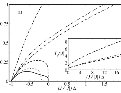
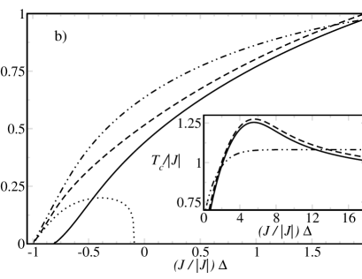
Figure 2: Critical temperature $T_{c}$ of the concurrence of the state of two qubits in the XXZ-model ($J\lessgtr 0$) for $2\leq N\leq 6$ as a function of anisotropy $\Delta$. Panel a) shows nearest neighbor qubits for $N=2$ (), $N=4$ () and $N=6$ (); next-to-nearest neighbor qubits for $N=4$ () and $N=6$ (); next-to-next-to-nearest neighbor qubits for $N=6$ (). Panel b) displays nearest neighbor qubits for $N=3$ ($J<0$: ; $J>0$: identical zero) and $N=5$ ($J<0$: ; $J>0$: ); next-to-nearest neighbor qubits for $N=5$ ($J<0$: ; $J>0$: identical zero). The insets give the dependence of these functions at larger values of $(J/\left|J\right|)\Delta$. Of course, the entanglement vanishes in the Ising model limit of (24), i.e., for $\left|\Delta\right|\rightarrow\infty$.

The transformation $J\rightarrow-J$ and $\Delta\rightarrow-\Delta$ leaves the critical temperature invariant for even $N$. If $\left|\psi\right\rangle$ is an eigenstate of $H(J,\Delta)$ with eigenvalue $E$ then $\left|\phi\right\rangle=A\left|\psi\right\rangle$ is the corresponding eigenstate of $H(-J,-\Delta)$ with the same eigenvalue and identical entanglement because $A$ is a local unitary transformation and entanglement is invariant under local unitary transformations. Thus the thermal density operators of both Hamiltonians are unitary equivalent and possess identical entanglement and critical temperatures. No such symmetry exists for odd $N$. Actually, for the states of nearest neighbor qubits ($N=3$) and next-to-nearest neighbor qubits ($N=5$) entanglement is only possible for $J<0$. In all considered cases the inequality $T_{c}(N,J<0)\geq T_{c}(N,J>0)$ is valid.

One observes in Fig. 2 that $T_{c}=0$ for $(J/\left|J\right|)\Delta\leq-1$ independently of $N$ and the choice of the two qubits. It is known from Takahashi (1999) that for all $N$, $J<0$ and $\Delta\geq 1$ the two eigenstates of the Hamiltonian (24) with $s=\pm\frac{N}{2}$ are ground states. These ground states are not entangled and they cause the thermal state to be unentangled for all temperatures. The same reasoning applies for even $N$, $J>0$ and $\Delta\leq-1$, because of the symmetries of the XXZ-model with periodic boundary conditions. The ground state may change at different $\Delta$ for odd $N$ and $J>0$ (e.g. at $\Delta\approx-0.809015$ considering the XXZ-model with $N=5$ and $J>0$).

Furthermore critical temperature of geometrically equivalent aligned qubits is decreasing with increasing $N$ for even $N$. This tendency is consistent with the dependence of concurrence on $N$ in the isotropic Heisenberg model with an applied external magnetic field (cf. Arnesen et al. (2001)).

V Analysis of an Experiment

Finally, the entanglement of the state of the quantum system in a NMR-experiment about quantum error correction Knill et al. (2001) is quantified in terms of concurrence, i-concurrence and 3-tangle. Five qubits are provided by different atoms in ¹³C labeled transcrotonic acid (synthesis and properties, see Knill et al. (2000)) solved in deuterated acetone.

One molecule can be approximately described by the one-dimensional spatial inhomogeneous XXZ-model including an external magnetic field because the coupling constants of non-neighboring qubits are much smaller than the coupling constants of nearest neighbor qubits (see Knill et al. (2001, 2000)). The Hamiltonian $H(J_{n},\Delta,\omega_{n})$ of this model reads

$$\begin{array}[]{rcl}H&=&\displaystyle\frac{1}{2}\sum\limits_{n=1}^{4}J_{n}\left(\sigma_{n}^{+}\sigma_{n+1}^{-}+\sigma_{n}^{-}\sigma_{n+1}^{+}+\frac{1}{2}\Delta\sigma_{n}^{z}\sigma_{n+1}^{z}\right)-\vspace{\jot}\\ &&\displaystyle\frac{1}{2}\sum\limits_{n=1}^{5}\omega_{n}\sigma_{n}^{z},\end{array}$$ (35)

where the coupling constants $J_{n}$ ($n=1,\ldots,4$) specify the inhomogeneous strength of nearest neighbor interaction, $\Delta$ determines the anisotropy in spin space and the effect of the external magnetic field is included in $\omega_{n}=\omega_{n}^{p}+\omega_{n}^{c}$ ($n=1,\ldots,5$) which are the sums of precession frequencies $\omega_{n}^{p}$ and chemical shifts $\omega_{n}^{c}$ for each individual qubit (data in Knill et al. (2001, 2000)). Of course, now open boundary conditions are applied.

The five-qubit code for quantum error correction is used to encode qubit $2$ in the experiment. The encoding is shown in Fig. 3.

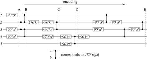
Figure 3: Encoding of qubit $2$ based on the five-qubit code. The horizontal lines represent the qubits. The gates denoted $\theta\sigma_{a}^{\alpha}$ and $180^{\circ}\sigma_{a}^{z}\sigma_{b}^{z}$ implement $e^{-\frac{i}{2}\theta\sigma_{a}^{\alpha}}$ and $e^{-\frac{i}{4}\pi\sigma_{a}^{z}\sigma_{b}^{z}}$, respectively. Here $\alpha\in\{x,y,z\}$ and $a,b\in\{1,2,3,4,5\}$.

The quantum system is in a highly mixed state, i.e., the coefficients of the density operator are close to the coefficients of the identity operator, because the experiment is performed at room temperature. In the beginning, the quantum system is prepared in a way that only molecules in the initial state $\left|11111\right\rangle$ give a signal on NMR measurements. Then one says that the quantum system is in the pseudo-pure state $\left|11111\right\rangle$ (Ref. Gershenfeld and Chuang (1997)). The pseudo-pure state $\left|11111\right\rangle$ is an eigenstate of the Hamiltonian (35) as well as the Hamiltonian including all interactions of qubits and the applied external magnetic field described in Knill et al. (2001, 2000). Furthermore it is an eigenstate of $S^{z}$. Thus going to a frame of reference that rotates around the $z$-axis does not change the density operator of the initial state (see (Becker, 2000, p. 287)).

The pseudo-pure state of the quantum system at several stages (A, B, C, D and E, cf. Fig. 3) during encoding was calculated by the product-operator-formalism (see (Becker, 2000, chapter 11)). Therefore, the conservation of the pseudo-purity of the state of the quantum system is assumed, i.e., there is no interaction between different molecules and encoding is implemented so quickly that no decoherence occurs. The results are given in Table 2 together with the expectation values $K_{n}^{z}$ and $K_{n}^{+}=\left(K_{n}^{-}\right)^{\star}$ (with $n=1$, $2$, $\ldots$, $5$).

Table 2: Pseudo-pure state $\left|\psi\right\rangle$ of the quantum system at several states during encoding. The expectation values $K_{n}^{z}$ and $K_{n}^{+}=\left(K_{n}^{-}\right)^{\star}$ (with $n=1$, $2$, $\ldots$, $5$) are given for each state. Notation: $\left|1_{x}\right\rangle:=\frac{1}{\sqrt{2}}\left(\left|1\right\rangle+\left|0\right\rangle\right)$, $\left|0_{x}\right\rangle:=\frac{1}{\sqrt{2}}\left(\left|1\right\rangle-\left|0\right\rangle\right)$, $\left|1_{y}\right\rangle:=\frac{1}{\sqrt{2}}\left(\left|1\right\rangle+i\left|0\right\rangle\right)$, $\left|0_{y}\right\rangle:=\frac{1}{\sqrt{2}}\left(\left|1\right\rangle-i\left|0\right\rangle\right)$, $\left|1_{z}\right\rangle:=\left|1\right\rangle$ and $\left|0_{z}\right\rangle:=\left|0\right\rangle$.

Position	$\left|\psi\right\rangle$	$K_{1}^{z}$	$K_{2}^{z}$	$K_{3}^{z}$	$K_{4}^{z}$	$K_{5}^{z}$	$K_{1}^{+}$	$K_{2}^{+}$	$K_{3}^{+}$	$K_{4}^{+}$	$K_{5}^{+}$
A	$\left|1_{x}1_{z}1_{x}0_{y}1_{z}\right\rangle$	$0$	$1$	$0$	$0$	$1$	$\frac{1}{2}$	$0$	$\frac{1}{2}$	$-\frac{i}{2}$	$0$
B	$\frac{1}{\sqrt{2}}\left|1_{y}1_{z}\right\rangle\otimes\left(\left|1_{z}1_{x}\right\rangle-\left|0_{z}0_{x}\right\rangle\right)\otimes\left|1_{z}\right\rangle$	$0$	$1$	$0$	$0$	$1$	$\frac{i}{2}$	$0$	$0$	$0$	$0$
C	$\frac{1}{\sqrt{2}}\left|1_{y}\right\rangle\otimes\left(\left|0_{x}1_{z}0_{z}\right\rangle+\left|1_{x}0_{z}1_{z}\right\rangle\right)\otimes\left|1_{z}\right\rangle$	$0$	$0$	$0$	$0$	$1$	$\frac{i}{2}$	$0$	$0$	$0$	$0$
D	$\frac{1}{2}\left|1_{y}\right\rangle\otimes\left[\left|0_{x}1_{z}\right\rangle\otimes\left(\left|1_{z}0_{x}\right\rangle+\left|0_{z}1_{x}\right\rangle\right)-i\left|1_{x}0_{z}\right\rangle\otimes\left(\left|1_{z}0_{x}\right\rangle-\left|0_{z}1_{x}\right\rangle\right)\right]$	$0$	$0$	$0$	$0$	$0$	$\frac{i}{2}$	$0$	$0$	$0$	$0$
E	$\frac{1}{2\sqrt{2}}\left\{\left|1_{x}\right\rangle\otimes\left[\left|0_{y}1_{z}\right\rangle\otimes\left(\left|1_{z}1_{z}\right\rangle+\left|0_{z}0_{z}\right\rangle\right)-\left|1_{y}0_{z}\right\rangle\otimes\left(\left|1_{z}1_{z}\right\rangle-\left|0_{z}0_{z}\right\rangle\right)\right]\right.+$ $\quad\left.i\left|0_{x}\right\rangle\otimes\left[\left|0_{y}0_{z}\right\rangle\otimes\left(\left|1_{z}0_{z}\right\rangle+\left|0_{z}1_{z}\right\rangle\right)-\left|1_{y}1_{z}\right\rangle\otimes\left(\left|1_{z}0_{z}\right\rangle-\left|0_{z}1_{z}\right\rangle\right)\right]\right\}$	$0$	$0$	$0$	$0$	$0$	$0$	$0$	$0$	$0$	$0$

It is straightforward to calculate the entanglement of one qubit with the remaining qubits by inserting these expectation values into Eq. (21). In this way it is easy to get a quick overview about the possible entanglement in the quantum system. Note that it is not appropriate to use Eqs. (4) and (15) or (22) here because the pseudo-pure state does not comply with the necessary $S^{z}$-symmetry in general.

The pseudo-pure state at the various stages is now discussed in detail: The initial state is not entangled. At position A, the state is not entangled as well. So far only local operations have been performed and these cannot create entanglement.

At position B, qubits $1$, $2$ and $5$ are not entangled but $C_{34}=1$. Actually, the state of qubits $3$ and $4$ at position B reads $\left|\psi\right\rangle_{34}=\frac{1}{2}\left(\left|11\right\rangle+\left|10\right\rangle-\left|01\right\rangle+\left|00\right\rangle\right)$ and it is conform to the Bell-states $\left|\psi^{\pm}\right\rangle$ and $\left|\phi^{\pm}\right\rangle=\frac{1}{\sqrt{2}}\left(\left|00\right\rangle\pm\left|11\right\rangle\right)$ up to a local unitary transformation.

At position C, only qubits $2$, $3$ and $4$ are entangled: $\bar{C}_{2-34}=\bar{C}_{3-24}=\bar{C}_{4-23}=\tau_{234}=1$, where the state of these qubits reads $\left|\psi\right\rangle_{234}=\frac{1}{2}\left(\left|110\right\rangle+\left|101\right\rangle-\left|010\right\rangle+\left|001\right\rangle\right)$. It is conform to the cat-state $\frac{1}{\sqrt{2}}\left(\left|000\right\rangle+\left|111\right\rangle\right)$ up to a local unitary transformation. Two out of these three qubits are not entangled as usual for a cat-state.

At position D, only qubit $1$ is not entangled. The state of the remaining qubits is conform to $\frac{1}{2}\left(\left|0110\right\rangle+\left|0101\right\rangle-i\left|1010\right\rangle+i\left|1001\right\rangle\right)$ up to a local unitary transformation. The analysis of qubits $2$, $3$, $4$ and $5$ shows no entanglement of the state of two of these qubits. The entanglement of a state of three qubits cannot be calculated because tracing off a qubit generates in general a mixed state and i-concurrence can only be applied to pure states. But it is $\bar{C}_{2-345}=\bar{C}_{3-245}=\bar{C}_{4-235}=\bar{C}_{5-234}=1$, $\bar{C}_{23-45}=1$ and $\bar{C}_{24-35}=\bar{C}_{25-34}=\sqrt{\frac{3}{2}}$.

At the end of the encoding sequence (position E), all qubits are entangled: $\bar{C}_{A-B}=1$ if $A$ indicates one arbitrary qubit and $B$ the remaining four qubits; $\bar{C}_{A-B}=\sqrt{\frac{3}{2}}$ if $A$ indicates two arbitrary qubits and $B$ the remaining three qubits. Again there is no entanglement of the state of two qubits and the entanglement of a state of three or four qubits cannot be quantified so far. These results coincide with the ones in Meyer and Wallach (2002). It was already pointed out there that all states in a certain fife-qubit error correction code subspace possess maximal global entanglement but vanishing concurrences.

Clearly, in this experiment, entanglement is created during encoding and it expands in a geometrical sense, i.e., the number of qubits involved in the entanglement increases with the progressing encoding sequence.

Unfortunately, it is not possible to quantify the entanglement of the state at positions D and E completely because of the lack of suitable measures. But all calculated i-concurrences exhibit their maximal values at position E. Thus it is a reasonable conjecture that an entanglement of four or less qubits does not exist there because entanglement cannot be shared arbitrarily (cf. Coffman et al. (2000)).

VI Summary

The entanglement measures concurrence, i-concurrence (for one or two qubits in one subsystem) and 3-tangle have been successfully expressed in terms of correlation functions. In addition, necessary and sufficient conditions for a positive concurrence have been formulated. These results have been used in the remaining paper because they can simplify calculations: The concurrence of eigenstates or the thermal state have been calculated analytically knowing only the energies of the eigenstates and their dependences on the parameters of the system. Furthermore potential quantum entanglement in a quantum system has been detected by the examination of spin expectation values.

A detailed analysis of concurrence and critical temperature in the XXZ-model with $2\leq N\leq 6$ qubits has been accomplished.

Finally, the entanglement of the state in a NMR-experiment has been discussed quantitatively. Different kinds of entanglement have been identified. This calculation shows the relevance of entanglement measures in actual experiments because they allow an analysis of the importance of entanglement for the quantum-algorithms. Despite the information, which is obtained with the available measures, further measures are needed for a complete insight.

The entanglement measures might be useful designing new experiments (possibly utilizing advanced types of qubits, e.g., spin cluster qubits Meier et al. (2003)) that set up states with different entanglement and prove or disprove the benefit of entanglement in different quantum-algorithms.

One of us (H.F.) thanks John Schliemann for useful discussions.

References

- Schrödinger (1935) E. Schrödinger, Die Naturwissenschaften 23, 807, 823, 844 (1935).
- Macchiavello et al. (2000) C. Macchiavello, G. M. Palma, and A. Zeilinger, eds., Quantum Computation and Quantum Information Theory (World Scientific Publishing Co. Pte. Ltd., 2000).
- Nielsen and Chuang (2001) M. A. Nielsen and I. L. Chuang, Quantum Computation and Quantum Information (Cambridge University Press, 2001).
- O’Connor and Wootters (2001) K. M. O’Connor and W. K. Wootters, Phys. Rev. A 63(5), 052302 (2001).
- Arnesen et al. (2001) M. C. Arnesen, S. Bose, and V. Vedral, Phys. Rev. Lett. 87(1), 017901 (2001).
- Wang et al. (2001) X. Wang, H. Fu, and A. I. Solomon, J. Phys. A 34(50), 11307 (2001).
- Wang (2002a) X. Wang, New J. Phys. 4, 11 (2002a).
- Wang and Zanardi (2002) X. Wang and P. Zanardi, Phys. Lett. A 301(1-2), 1 (2002).
- Wang (2002b) X. Wang, Phys. Rev. A 66(4), 044305 (2002b).
- Schliemann (2002) J. Schliemann, quant-ph/0212114 (2002).
- Gunlycke et al. (2001) D. Gunlycke, V. M. Kendon, V. Vedral, and S. Bose, Phys. Rev. A 64(4), 042302 (2001).
- Kamta and Starace (2002) G. L. Kamta and A. F. Starace, Phys. Rev. Lett. 88(10), 107901 (2002).
- Osterloh et al. (2002) A. Osterloh, L. Amico, G. Falci, and R. Fazio, Nature 416, 608 (2002).
- Osborne and Nielsen (2002) T. J. Osborne and M. A. Nielsen, Phys. Rev. A 66(3), 032110 (2002).
- Bose and Chattopadhyay (2002) I. Bose and E. Chattopadhyay, Phys. Rev. A 66(6), 062320 (2002).
- Vidal et al. (2002) G. Vidal, J. I. Latorre, E. Rico, and A. Kitaev, quant-ph/0211074 (2002).
- Latorre et al. (2003) J. I. Latorre, E. Rico, and G. Vidal, quant-ph/0304098 (2003).
- Meyer and Wallach (2002) D. A. Meyer and N. R. Wallach, J. Math. Phys. 43(9), 4273 (2002).
- Hill and Wootters (1997) S. Hill and W. K. Wootters, Phys. Rev. Lett. 78(26), 5022 (1997).
- Wootters (1998) W. K. Wootters, Phys. Rev. Lett. 80(10), 2245 (1998).
- Rungta et al. (2001) P. Rungta, V. Bužek, C. M. Caves, M. Hillery, and G. J. Milburn, Phys. Rev. A 64(4), 042315 (2001).
- Coffman et al. (2000) V. Coffman, J. Kundu, and W. K. Wootters, Phys. Rev. A 61(5), 052306 (2000).
- Knill et al. (2001) E. Knill, R. Laflamme, R. Martinez, and C. Negrevergne, Phys. Rev. Lett. 86(25), 5811 (2001).
- Takahashi (1999) M. Takahashi, Thermodynamics of one-dimensional solvable models (Cambridge University Press, 1999).
- Yang and Yang (1966) C. N. Yang and C. P. Yang, Phys. Rev. 147(1), 303 (1966).
- Orbach (1958) R. Orbach, Phys. Rev. 112(2), 309 (1958).
- Stroganov (2001) Y. Stroganov, J. Phys. A 34(13), L179 (2001).
- Nielsen (1998) M. A. Nielsen, Quantum Information Theory, Ph.D. thesis, The University of New Mexico Albuquerque (1998), quant-ph/0011036.
- Knill et al. (2000) E. Knill, R. Laflamme, R. Martinez, and C.-H. Tseng, Nature 404, 368 (2000).
- Gershenfeld and Chuang (1997) N. A. Gershenfeld and I. L. Chuang, Science 275, 350 (1997).
- Becker (2000) E. D. Becker, High Resolution NMR (Academic Press, 2000).
- Meier et al. (2003) F. Meier, J. Levy, and D. Loss, Phys. Rev. Lett. 90(4), 047901 (2003).