Translational Entanglement of Dipole-Dipole Interacting Atoms in Optical Lattices

Abstract

We propose and investigate a realization of the position- and momentum-correlated Einstein-Podolsky-Rosen (EPR) states [Phys. Rev. 47, 777 (1935)] that have hitherto eluded detection. The realization involves atom pairs that are confined to adjacent sites of two mutually shifted optical lattices and are entangled via laser-induced dipole-dipole interactions. The EPR “paradox” with translational variables is then modified by lattice-diffraction effects, and can be verified to a high degree of accuracy in this scheme.

The ideal Einstein-Podolsky-Rosen (EPR) EPR state of two particles—1 and 2, is, respectively, represented in their coordinates or momenta (in one dimension), as follows,

$$\langle x_{1},x_{2}|\psi_{\rm EPR}\rangle = \delta(x_{1}-x_{2}),$$ (1)

$$\langle p_{1},p_{2}|\psi_{\rm EPR}\rangle = \delta(p_{1}+p_{2}).$$ (2)

The “paradox” is in the fact that given the measured values of $x_{1}$ or $p_{1}$ of particle 1, one can predict the measurement result of $x_{2}$ or $p_{2}$, respectively, with arbitrary precision, unlimited by the Heisenberg relation $\Delta x_{2}\Delta p_{2}\geq\hbar/2$. In other words, the ideal EPR state is fully entangled in the continuous translational variables of the two particles. Approximate versions of this translational EPR state, wherein the $\delta$-function correlations are replaced by finite-width distributions, have been shown to characterize the quadratures of the two optical-field outputs of parametric downconversion Reid ; Ou and allow for optical continuous-variable teleportation BraunsteinKimble . More recently, translational EPR correlations have been analyzed between dissociation fragments of homonuclear diatoms opa01 , whereas interacting atoms in Bose-Einstein condensates have been shown to possess translational–internal correlations CiracZoller . Yet the fact remains that the original EPR state has eluded detection for nearly 70 years. Our goal is twofold: (i) propose an experimentally feasible scheme for the creation of translational EPR correlations between cold atoms that are confined in optical lattices Hamann and coupled by laser-induced dipole-dipole interactions (LIDDI) Thirun ; induceddd ; duncan ; (ii) study the qualitative modifications of such correlations due to particle diffraction in lattices, which have been hitherto unexplained. The LIDDI has been proposed as a means of two-atom entanglement via their internal states, for quantum logic applications Brennen . The ability of LIDDI to influence the spatial and momentum distributions of cold atoms in cavities DebKurizki , traps and condensates TrapsConds , has been investigated extensively.

To realize and measure the EPR translational correlations of material particles, one must be able to accomplish several challenging tasks: (a) switch on and off the entangling interaction; (b) confine their motion to single dimension, and (c) infer and verify the dynamical variables of particle 2 at the time of measurement of particle 1. The latter requirement is particularly hard for free particles, since by the time we complete the prediction for particle 2, its position will have changed. In opa01 we suggested to overcome these hurdles by transforming the wavefunction of a flying (ionized) atom by an electrostatic/magnetic lens onto the image plane, where its position corresponds to what it was at the time of the diatom dissociation. In this Letter we propose a different solution: (a) controlling the diatom formation and dissociation by switching on and off the LIDDI; (b) controlling the motion and effective masses of the atoms and the diatom by changing the intensities of the lattice fields.

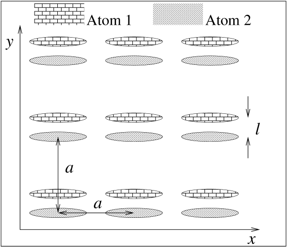
Figure 1: Proposed scheme of the translational EPR: two overlapping optical lattices displaced from each other in the $y$ direction by $l$, are sparsely occupied by two kinds of atoms. Each of the two kinds of atoms feels a different lattice; the shaded regions depict the energy minima (potential wells) of the lattices.

System specification: Let us assume two overlapping optical lattices with the same lattice constant $a$, as in Fig. 1. The lattices are very sparsely occupied by two kinds of atoms, each kind interacting with only one of the two lattices. This can be realized, e.g., by assuming two different internal (say, hyperfine) states of the atoms Brennen . For both lattices, the $y$ and $z$ directions are very strongly confining (realized by strong laser fields), whereas in the $x$ direction the lattice can be varied from moderately to weakly confining. Thus, the motion of each particle is confined to the $x$ direction. For each direction we assume that only the lowest vibrational energy band is occupied. Initially, the potential minima of the lattices are displaced from each other by an amount $l\ll a$ in the $y$ direction. This enables us to couple the atoms of the two lattices, along $y$ using an auxiliary laser to induce the LIDDI. We assume the auxiliary laser to be a linearly polarized traveling wave with wavelength $\lambda_{\rm C}$, moderately detuned from an atomic transition that differs from the one used to trap the atoms in the lattice. The auxiliary laser propagates in the $x$ direction and its electric field is polarized in the $y$ direction. The LIDDI potential for two identical atoms has the form Thirun

$$V_{\rm dd}=-V_{\rm C}F_{\theta}(kR),\ \quad F_{\theta}(kR)=\cos\left(kR\cos\theta\right)$$

$$\times\left\{(2\!-\!3\cos^{2}\theta)\left[\frac{\cos kR}{(kR)^{3}}\!+\!\frac{\sin kR}{(kR)^{2}}\right]\!+\!\cos^{2}\theta\frac{\cos kR}{kR}\right\}.$$ (3)

Here $V_{\rm C}=\alpha^{2}k^{3}I_{\rm C}/(4\pi\epsilon_{0}^{2}c)$, where $k=2\pi/\lambda_{\rm C}$, $I_{\rm C}$ is the coupling laser intensity, and the atomic dynamic polarizability is $\alpha=2\omega_{A}|\mu|^{2}/[\hbar(\omega_{A}^{2}-\omega^{2})]$, $\mu$ being the dipole moment element, $\omega_{A}$ the atomic transition frequency, and $\omega=kc$. The position-dependent part $F_{\theta}(kR)$ is a function of $R$, the distance between the atoms, and $\theta$, the angle between the interatomic axis and the wavevector of the coupling laser. Since $l\ll 2a$, $V_{\rm dd}(R)$ has a pronounced minimum for atoms located at the nearest sites, $R\simeq l$, where $V_{\rm dd}(R)\simeq-V_{\rm C}(\lambda_{\rm C}/l)^{3}/(4\pi^{3})$. Under these assumptions, we can treat the system as consisting of pairs of “tubes”, that are oriented along $x$, either empty or occupied. Only atoms within adjacent tubes are appreciably attracted to each other along $y$, due to the LIDDI.

EPR states: We now focus on the subensemble of tube-pairs in which each tube is occupied by exactly one atom. In the absence of LIDDI, the state of each atom can be described in terms of the Wannier functions $|\chi_{j}\rangle$ Wannier that are localized at lattice sites with index $j$ and may hop to the neighboring site at the rate $V_{\rm hop}/\hbar$, where $V_{\rm hop}=\langle\chi_{j}|\hat{H}_{\rm lat}|\chi_{j+1}\rangle$, and $\hat{H}_{\rm lat}$ is the lattice Hamiltonian. In a 1D lattice, $\hat{H}_{\rm lat}=(U_{0}/2)\cos\left(2\pi x/a\right)+\hat{p}_{x}^{2}/(2m)$, $m$ being the atomic mass. The hopping rate is related to the energy bandwidth of the lowest lattice band $V_{B}$ by $V_{B}\approx 4|V_{\rm hop}|$ (for exact expressions see Slater ). For a shallow lattice potential ($U_{0}\lesssim 15E_{\rm rec}$) we may use the approximate formula $V_{\rm hop}\approx E_{\rm rec}\exp(-0.26\ U_{0}/E_{\rm rec})$, where the recoil energy is $E_{\rm rec}=2\pi^{2}\hbar^{2}/(m\lambda_{\rm L}^{2})$.

Let us switch on the LIDDI, so that $|V_{\rm hop}|\ll|V_{\rm dd}|$. Then the ground state of such a tightly bound diatom can be approximated by $|\psi_{0}\rangle\propto\sum_{j}|\chi_{j}^{(1)}\rangle|\chi_{j}^{(2)}\rangle$. This means that when particle 1 is found at the $j$th site of lattice 1, then particle 2 is found at the $j$th site of lattice 2, with position dispersion given by the half-width $\sigma$ of the atomic (Gaussian-like) Wannier function in the lowest band, $\sigma^{2}=\hbar\lambda_{\rm L}/(4\pi\sqrt{mU_{0}})$. To next order in $V_{\rm hop}/V_{\rm dd}$, the nonzero probability of atoms to be located at more distant sites changes the diatomic position (separation) dispersion to $\Delta x_{-}^{2}\approx\sigma^{2}+2a^{2}\left(\frac{V_{\rm hop}}{V_{\rm dd}}\right)^{2}$.

The states of the tightly bound diatom form a separate band whose bandwidth is $V_{B}^{\rm(2at)}\approx 4|V_{\rm hop}^{\rm(2at)}|$, below the lowest atomic vibrational band. The diatomic hopping potential $V_{\rm hop}^{\rm(2at)}$ can be found by assuming that the two atoms consecutively hop to their neighboring sites, i.e., the state change $|\chi_{j}^{(1)}\rangle|\chi_{j}^{(2)}\rangle\to|\chi_{j+1}^{(1)}\rangle|\chi_{j+1}^{(2)}\rangle$ is realized either via $|\chi_{j}^{(1)}\rangle|\chi_{j}^{(2)}\rangle\to|\chi_{j+1}^{(1)}\rangle|\chi_{j}^{(2)}\rangle\to|\chi_{j+1}^{(1)}\rangle|\chi_{j+1}^{(2)}\rangle$, or via $|\chi_{j}^{(1)}\rangle|\chi_{j}^{(2)}\rangle\to|\chi_{j}^{(1)}\rangle|\chi_{j+1}^{(2)}\rangle\to|\chi_{j+1}^{(1)}\rangle|\chi_{j+1}^{(2)}\rangle$. By adiabatic elimination of the higher-energy intermediate states one obtains $V_{\rm hop}^{\rm(2at)}\approx 2V_{\rm hop}^{2}/V_{\rm dd}$.

To realize a momentum anti-correlated EPR state, the temperature of the system must satisfy $k_{B}T\ll V_{B}^{\rm(2at)}$. The dependence of the momentum anti-correlation on temperature is given by $\Delta p_{+}^{2}/(2m_{\rm eff}^{\rm(2at)})\approx\frac{1}{2}k_{B}T$, where we have introduced the sum-momentum spread $\Delta p_{+}$ and (analogously to atomic effective mass Slater ) the two-atom effective mass $m_{\rm eff}^{\rm(2at)}=\frac{2\hbar^{2}}{V_{B}^{\rm(2at)}a^{2}}\approx\frac{\hbar^{2}|V_{\rm dd}|}{4V_{\rm hop}^{2}a^{2}}$. We then obtain $\Delta p_{+}^{2}\approx\frac{\hbar^{2}|V_{\rm dd}|}{4V_{\rm hop}^{2}a^{2}}k_{B}T$.

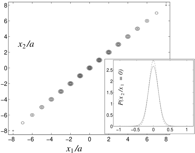
Figure 2: Joint probability distribution of the positions of two lithium atoms in adjacent optical lattices, prepared in a diatom state as specified in the text, using the ground state of the external harmonic potential with half-width of $\sigma_{E}=6a$ and temperature of 10 nK. Inset: Position probability of atom 2 in the state above, conditional on atom 1 being measured at site 0 (full line). Dashed line: Gaussian approximation of the Wannier function with the half-width $\sigma=0.14a$.

Although the values $\Delta x_{-}^{2}$ and $\Delta p_{+}^{2}$ estimated above refer to the respective peak widths, they principally differ from the position and momentum uncertainties of free particles: due to the lattice periodicity, the position and momentum distributions have generally a multi-peak structure. The two-particle joint position distribution of the ground state is a chain of peaks of half-width $\sigma$ separated by $a$; the peaks are located along the line $x_{2}=x_{1}$ (Fig. 2). The corresponding joint momentum distribution spreads over an area of half-width $\hbar/(2\sigma)$ and consists of ridges in the direction $p_{2}=-p_{1}$. These ridges are separated by $2\pi\hbar/a$, and for a lattice of $N$ sites, the half-width of each ridge is $\pi\hbar/(Na)$ (Fig. 3).

To evaluate how “strong” the EPR effect is, we compare the product of the half-widths of the position and momentum peaks in the tightly bound diatom state described above with the limit of the Heisenberg uncertainty relations, $\Delta x\Delta p\geq\hbar/2$, defining the parameter $s$ opa01 :

$$s=\frac{\hbar}{2\Delta x_{-}\Delta p_{+}}.$$ (4)

A value of $s$ higher than 1 indicates the occurrence of the EPR effect; the higher the value of $s$, the stronger the effect. Strictly speaking, because of the multi-peak momentum distribution, one should not use the original form of Heisenberg uncertainty relations but a more general relation, as discussed, e.g., in Uffink , that distinguishes the uncertainty of a few narrow peaks from that of a single broad peak. However, even the simple half-width of the peaks is a useful measure of the EPR effect. In order to maximize $s$, we must adhere to the trade-off between making $\Delta x_{-}$ as small as possible, by decreasing $|V_{\rm hop}/V_{\rm dd}|$, and making $\Delta p_{+}$ as small as possible, by increasing $|V_{\rm hop}/V_{\rm dd}|$. The optimum value of $s$ generally depends on the lowest available temperature of the diatom, as detailed below.

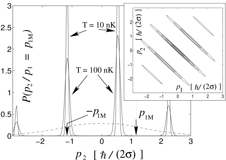
Figure 3: Conditional probability of the momentum of atom 2 after the momentum of atom 1 has been measured for lithium diatoms prepared as in the text (the measured value $p_{1}=p_{1{\rm M}}$ is indicated with an arrow). The dashed line corresponds to the marginal probability distribution of momentum $p_{2}$ irrespective of the momentum of atom 1 at the temperature $T=100$ nK. The half-width of each peak is equal to $1/s$ of Eq. (4). Inset: joint probability distribution of the atomic momenta in the state above with $T=100$ nK.

EPR state preparation: Cooling down the diatomic system to prepare the EPR state is a non-trivial task. We suggest to attack the problem by a three-step approach. (i) Let us switch off both the LIDDI and the $x$-lattices, switch on an external, shallow, harmonic potential in the $x$ direction, and cool the $x$-motion of the atoms down to the ground state of the external potential. The width $\sigma_{E}$ of the ground state should be several times the lattice constant; it is related to the desired momentum anti-correlation by $\sigma_{E}\approx\hbar/(\sqrt{2}\Delta p_{+})$. The temperature must be $T\ll\hbar^{2}/(4mk_{B}\sigma_{E}^{2})$. (ii) A weak lattice potential in the $x$-direction is then slowly switched on, so that the state becomes $\approx(\sum_{j}\alpha_{j}|\chi_{j}^{(1)}\rangle)(\sum_{l}\alpha_{l}|\chi_{l}^{(2)}\rangle)=\sum_{j}\alpha_{j}^{2}|\chi_{j}^{(1)}\rangle|\chi_{j}^{(2)}\rangle+\sum_{j\neq l}\alpha_{j}\alpha_{l}|\chi_{j}^{(1)}\rangle|\chi_{l}^{(2)}\rangle$, where the coefficients $\alpha_{j}\sim\exp[-(j-j_{0})^{2}a^{2}/(4\sigma_{E}^{2})]$ are Gaussians localized around the minimum of the external potential. (iii) We switch on the LIDDI and change the sign of the external potential, from attractive to repulsive, acting to remove the particles from the lattice. The two parts of the wavefunction would behave in different ways. The paired atoms, corresponding to the part of the wavefunction $\sum_{j}\alpha_{j}^{2}|\chi_{j}^{(1)}\rangle|\chi_{j}^{(2)}\rangle$, move slowly because of their large effective mass $m_{\rm eff}^{\rm(2at)}$, whereas single (unpaired) atoms, because of their smaller effective mass, $m_{\rm eff}\ll m_{\rm eff}^{\rm(2at)}=|V_{\rm dd}|/(2V_{\rm hop})m_{\rm eff}$, are ejected out of the lattice and separated from the diatoms as glumes from grains. The paired atoms remaining in the lattice are then in the state $\sim\exp[-(j-j_{0})^{2}a^{2}/(2\sigma_{0}^{2})]|\chi_{j}^{(1)}\rangle|\chi_{j}^{(2)}\rangle$ wherein positions are correlated with uncertainty $\Delta x_{+}\approx\sigma_{E}/\sqrt{2}$ and momentum uncertainty $\Delta p_{+}\approx\hbar/\Delta x_{+}$. At higher temperatures the atoms are not cooled to the ground state of the external potential and the momentum anti-correlation becomes $\Delta p_{+}\approx\hbar/\{\sqrt{2}\sigma_{E}\tanh[\hbar^{2}/(2\sigma_{E}^{2}mk_{B}T)]\}$. The parameter $s$ of Eq. (4) can then be estimated as

$$s\approx\frac{\sigma_{E}}{\sqrt{2}\sigma}\tanh\left[\frac{1}{\pi^{2}}\left(\frac{a}{\sigma_{E}}\right)^{2}\frac{E_{\rm rec}}{k_{B}T}.\right]$$ (5)

This equation enables us to select the optimum external harmonic potential (specified here by $\sigma_{E}$) such that the parameter $s$ is maximized, under the constraint of the lowest achievable temperature $T$.

The small effective mass of unpaired atoms allows us to cool them individually, restricting their cooling to temperatures higher than that corresponding to the bottom of the diatomic band. The price is, however, that most of the atoms are discarded and only a small fraction remains in the diatom state. Specifically, out of the total number of tube pairs occupied by two atoms, a fraction of $\sim a/\sigma_{E}$ will remain in the bound diatom state. The different behavior of the paired vs. unpaired atoms in a periodic potential is a sparse-lattice analogy of the Mott-insulator vs. superfluid state of the fully occupied lattice, recently observed in Ref. Greiner .

Measurements: After preparing the system in the EPR state, one can test its properties experimentally. To this end we may increase the lattice potential $U_{0}$, switch off the field inducing the LIDDI, and separate the two lattices by changing the laser-beam angles. By increasing $U_{0}$, the atoms lose their hopping ability and their quantum state is “frozen” with a large effective mass: the bandwidth $V_{B}$ decreases exponentially with $U_{0}$ and the effective mass increases exponentially, so that the atoms become too “heavy” to move. One has then enough time to perform measurements on each of them.

The atomic position can be measured by detecting its resonance fluorescence. After finding the site occupied by atom 1, one can infer the position of atom 2. If this inference is confirmed in a large ensemble of measurements, it would suggest that there is an “element of reality” EPR corresponding to the position of particle 2. The atomic momentum can be measured by switching off the $x$-lattice potential of the measured atom (thus bringing it back to its “normal” mass $m$): the distance traversed by the atom during a fixed time is proportional to its momentum. One can test the EPR correlations between the atomic distributions occupying the two lattices: a large number of pairs would be tested in a single run. The correlations in $x$ and anti-correlations in $p$ would be observed by matching the distribution histograms measured on particles from the two lattices.

Example: We consider two lithium atoms in two lattices with $\lambda_{\rm L}=$ 323 nm (corresponding to the transition 2s–3p) and a dipole-dipole coupling field of $\lambda_{\rm C}=$ 670.8 nm (transition 2s–2p). The field intensities are $I_{\rm L}=$ 0.35 W/cm² and $I_{\rm C}=$ 0.1 W/cm², and the field detunings are $\delta_{\rm L}=50\gamma_{\rm L}$, $\delta_{\rm C}=100\gamma_{\rm C}$, the decay rates being $\gamma_{\rm L}=1.2\times 10^{6}$ s^-1, and $\gamma_{\rm C}=3.7\times 10^{7}$ s^-1. The two lattices are displaced by $l=$ 40 nm. From these values we get the lattice potential $U_{0}=7.42E_{\rm rec}$, the dipole-dipole potential of the nearest atoms $V_{\rm dd}=-2.16E_{\rm rec}$, and the hopping potential $V_{\rm hop}=-0.0355E_{\rm rec}$. The two-particle hopping potential is then $V_{\rm hop}^{\rm(2at)}\approx-0.0012E_{\rm rec}$ and the ratio of effective masses of a diatom and a of single atom is $m_{\rm eff}^{\rm(2at)}/m_{\rm eff}\approx 30$. The position uncertainty of atom 2, after position measurement of atom 1, is then $\Delta x_{-}\approx\sigma=0.136a=22$ nm (see Fig. 2). The correlated pairs are prepared by first cooling independent atoms in an external harmonic potential with the ground-state half-width of $\sigma_{E}=6a$ (frequency of 1.2 kHz $\sim 33$ nK). After the unpaired atoms are removed from the lattice, we calculate the momentum distribution for two different temperatures, 10 nK and 100 nK. The conditional probability of momentum $p_{2}$ of particle 2, provided that the momentum of particle 1 was measured as $p_{1M}$ is plotted in Fig. 3. The resulting half-widths of the peaks can be used to find the parameter $s$; we have $s\approx 30$ for $T=$ 10 nK, and $s\approx 11$ for $T=$ 100 nK. Note that in current optical experiments Ou $s\lesssim 4$.

To sum up, the proposed scheme is based on the adaptation of existing techniques (optical trapping, cooling, controlled dipole-dipole interaction) to the needs of atom-atom translational entanglement. The most important feature of the scheme is the manipulation of the effective mass, both for the EPR-pair preparation (by separating the “light” unpaired atoms from the “heavy” diatoms) and for their detection (by “freezing” the atoms in their initial state so that their EPR correlations are preserved long enough). This scheme has the capacity of demonstrating the original EPR effect for positions and momenta, as discussed in the classic paper EPR . A novel element of the present scheme is the extension of the EPR correlations to account for lattice-diffraction effects. Applications of this approach to matter teleportation opa01 and quantum computation with continuous variables comput can be envisioned. The fact that our system represents a blend of continuous and discrete variables may be utilized for quantum information-processing (to be discussed elsewhere).

Acknowledgments: We acknowledge the support of the US-Israel BSF, Minerva and the EU Networks QUACS and ATESIT.

References

- (1) A. Einstein, B. Podolsky, and N. Rosen, Phys. Rev. 47, 777 (1935).
- (2) M.D. Reid and P.D. Drummond, Phys. Rev. Lett. 60, 2731 (1988).
- (3) Z.Y. Ou, S.F. Pereira, H.J. Kimble, and K. C. Peng, Phys. Rev. Lett. 68, 3663 (1992).
- (4) S.L. Braunstein and H.J. Kimble, Phys. Rev. Lett. 80, 869 (1998).
- (5) T. Opatrný and G. Kurizki, Phys. Rev. Lett. 86, 3180 (2001).
- (6) L.-M. Duan et al., Phys. Rev. Lett. 85, 3991 (2000); H. Pu and P. Meystre, ibid 85, 3987 (2000).
- (7) S.E. Hamann et al., Phys. Rev. Lett. 80, 4149 (1998); A. Fioretti et al., Phys. Rev. Lett. 80, 4402 (1998).
- (8) T. Thirunamachandran, Molecular Physics 40, 393 (1980).
- (9) M.M. Burns et al., Science 249, 749 (1990); P.W. Milonni and A. Smith, Phys.Rev. A 53, 3484 (1996).
- (10) D. O’Dell et al., Phys.Rev.Lett. 84, 5687 (2000); S. Giovanazzi et al., Phys. Rev. A 63, 031603(R) (2001).
- (11) G.K. Brennen et al., Phys. Rev. Lett. 82, 1060 (1999); I.H. Deutsch and G.K. Brennen Fortschr. Phys. 48, 925 (2000); O. Mandel et al., cond-mat/0301169 (2003).
- (12) B. Deb and G. Kurizki, Phys. Rev. Lett. 83, 714 (1999).
- (13) G. Kurizki et al., Lecture Notes in Physics, vol. 601, p. 388 (Springer, 2002); S. Giovanazzi, D. O’Dell, and G. Kurizki, Phys. Rev. Lett. 88, 130402 (2002).
- (14) J.C. Slater, Phys. Rev. 87, 807 (1952).
- (15) G.H. Wannier, Phys. Rev. 52, 191 (1937).
- (16) J. Hilgevoord and J.B.M. Uffink, Phys. Lett. A 95, 474 (1983); J.B.M. Uffink and J. Hilgevoord, ibid 105, 176 (1984); Found. Phys. 15, 925 (1985).
- (17) M. Greiner et al., Nature 415, 39 (2002).
- (18) S. Lloyd and J.-J.E. Slotine, Phys. Rev. Lett. 80, 4088 (1998), S.L. Braunstein, Nature 394, 47 (1998); S. Lloyd and S.L. Braunstein, Phys. Rev. Lett. 82, 1784 (1999).