Rényi extrapolation of Shannon entropy

Abstract.

Relations between Shannon entropy and Rényi entropies of integer order are discussed. For any $N$–point discrete probability distribution for which the Rényi entropies of order two and three are known, we provide an lower and an upper bound for the Shannon entropy. The average of both bounds provide an explicit extrapolation for this quantity. These results imply relations between the von Neumann entropy of a mixed quantum state, its linear entropy and traces.

ver. 2 with corrigendum added,   February 17, 2005

1. Introduction

We are going to analyze discrete probability distributions ${\vec{x}}=\{x_{1},..x_{N}\}$, which consist of non–negative numbers summing to unity. $\sum_{i=1}^{N}x_{i}=1$. To characterize quantitatively such probability vectors one uses Shannon (information) entropy [1]

(1) $$H({\vec{x}}):=-\sum_{i=1}^{N}x_{i}\ln x_{i}$$

where we adopt the convention that $0\ln 0=0$, if necessary.

The Shannon entropy is distinguished by several unique properties [2], but it is often convenient to introduce generalized Rényi entropies [3] parametrized by a continuous parameter $q$,

(2) $$H_{q}({\vec{x}}):=\frac{1}{1-q}\ln\Bigl{[}\sum_{i=1}^{N}x_{i}^{q}\Bigr{]}.$$

The Rényi entropies are well defined for positive $q\neq 1$, but is is not difficult to show that for any probability distribution $\vec{x}$ one has $\lim_{q\to 1}H_{q}({\vec{x}})=H({\vec{x}})$. For consistency the Shannon entropy $H$ will thus be denoted by $H_{1}$. This method of generalizing the Shannon entropy is by far not the only one – for reviews of other generalizations see books by Kapur [4] and Arndt [5].

In this work we discuss relations between Rényi entropies of different orders, and in particular between $H_{1}$, $H_{2}$ and $H_{3}$. Physical motivation for such a study is twofold. First, we may not know the entire vector $\vec{x}$, but only a few of its $L_{q}$ norms, so knowing the Renyi entropies, say $H_{2}$ and $H_{3}$ we want to estimate the unknown Shannon entropy $H_{1}$. Such a situation occurs if one studies an $N$ dimensional quantum mechanical mixed state $\rho$ according to the scheme recently proposed by P. Horodecki et al. [6, 7] and measures directly the traces Tr$\rho^{k}$ for $k=2,3,...M$. If $M<N$ the entire spectrum of $\rho$ remains unknown, and it is not possible to find its von Neumann entropy, $S(\rho)=-{\rm Tr}\rho\ln\rho$, (i.e. the Shannon entropy of the spectrum), but the generalized Renyi entropies $H_{k}$, including the linear entropy, which is a function of $H_{2}$ may be readily obtained. Similar problems arise in many different branches of physics, for instance by the study of the statistics between particles created in high–energy collisions [8, 9]. Measuring probabilities of that two independent collisions give rise to the same distribution of particles allows one to obtain the Rényi entropy $H_{2}$, but not directly the Shannon entropy $H_{1}$.

Another reason to study relations between $H_{1}$ and $H_{2}$ has been provided by the work by Pipek and Varga [10]. They assumed that both these quantities are known, and observed that their difference, $S_{str}:=H_{1}-H_{2}$ called structural entropy, provides an important characterization of the analyzed probability vector $\vec{x}$. For instance, an increase of the structural entropy charactering an eigenstate of a tight binding model indicates the Anderson transition. Several other applications of structural entropy include also quantum chemistry and statistical analysis of quantum spectra, (see [11] and references therein).

The von Neumann entropy of a mixed state obtained by partial trace of a bi–partite pure state, $\rho={\rm Tr}_{B}(|\psi\rangle\langle\psi|)$, measures the degree of entanglement of the pure state $|\psi\rangle$. Alternatively one can measure the entanglement by generalized entropies (see e.g. [12]), so relations between entropies analyzed in this work provide bounds between different measures of entanglement. This very point has recently been discussed in the paper by Wei et al. [13], which provides an additional motivation for the present work.

This paper is ogranized as follows. In section 2 the basic properties of the Rényi entropies are reviewed. In section 3 we present recent results of Topsøe and Harremoës [14, 15], which allow us to propose lower and upper bounds on the Shannon entropy obtained out of the Rényi entropies of order two and three, provided the length $N$ of the vector is known. They are derived in section 4, while in section 5 we propose and analyze en estimation of the Shannon entropy.

2. Shannon and Rényi entropies

Consider a random variable $\xi$ attaining not more than $N$ different values with probabilities $x_{i}$, $i=1,\dots,N$. Such discrete probability distribution $P$ may be cahracterized by the Shannon entropy (1) or generalized Rényi entropies (2).

All generalized entropies $H_{q}$ vary from zero for a certain event (the distribution $Q_{1}:=\{1,0,...,0\}$) to $\ln N$, for the uniform distribution, (the distribution $Q_{N}:=\{1/N,1/N,...,1/N\}$). For the distributions with $k$ equal elements, $Q_{k}:=\{1/k,...,1/k,0,...,0\}$, the entropies admit intermediate values, $\ln k$.

The Rényi entropy $H_{q}$ converges to the Shannon entropy in the limit $q\to 1$. It is also useful to express the Shannon entropy as the limit of the derivative,

(3) $$H({\vec{x}})=-\lim_{q\to 1}\frac{\partial[(1-q)\exp\bigl{(}H_{q}({\vec{x}})\bigr{)}]}{\partial q}.$$

Some special cases of $H_{q}$ are of special interest. For $q=2$ we have $H_{2}(\vec{x})=-\ln[\sum_{i=1}^{N}x_{i}^{2}]$. The Rényi entropy of order two, called extension entropy [10], is closely related to the inverse participation ratio,

(4) $$R({\vec{x}}):=\frac{1}{\sum_{i=1}^{N}x_{i}^{2}}=\exp[H_{2}({\vec{x}})].$$

This quantity characterizes the ”effective number of different events” which the stochastic variable may admit, and varies from unity for $Q_{1}$, to $N$ for the uniform distribution $Q_{N}$. Another quantity $r=1/R=\sum_{i=1}^{N}x_{i}^{2}$, called index of coincidence [15], in quantum mechanical problems is called purity, since the larger $r$ the more pure, the state it describes. The quantity $L:=1-r=1-\exp(-H_{2})$ is called linear entropy since in analogy to Shannon entropy it achieves its maximum for the uniform distribution $Q_{N}$.

In the case $q=0$ the Rényi entropy is a function of the number $m$ of positive components of the vector, $H_{0}(\vec{x})=\ln m$. In the limit $q\to\infty$ we obtain a quantity analogous to the Chebyshev norm: $H_{\infty}=-\ln x_{\rm max}$, where $x_{\rm max}$ is the largest component of $\vec{x}$.

The Rényi entropy (2) is a sum of $N$ terms so for any finite $N$ the function of $H_{q}$ on $q$ is differentiable. The functional dependence of the Rényi entropy on its parameter was investigated in detail by Back and Schlögl [16]). Making use of the fact that the function $x^{s}$ is convex for $s>1$ and concave for $0\leq s\leq 1$ they have proved several inequalities, which we recall in the case $q>0$,

(5) $$\frac{\partial}{\partial q}H_{q}\leq 0,$$

(6) $$\frac{\partial}{\partial q}\frac{q-1}{q}H_{q}\geq 0,$$

(7) $$\frac{\partial}{\partial q}(1-q)H_{q}\leq 0,$$

(8) $$\frac{\partial^{2}}{\partial q^{2}}(1-q)H_{q}\geq 0.$$

The first inequality (5) means that the Rényi entropy is a non increasing function of its parameter,

(9) $$H_{q}({\vec{x}})\geq H_{s}({\vec{x}})\qquad{\rm for\qquad any}\qquad s>q$$

and this statement is valid also for infinite probability vectors and the cases of nondifferentiable $H_{q}$ [16]. Hence the structural entropy $S_{str}:=H_{1}-H_{2}$ is non–negative [10].

Inequality (8) implies that the dependence of the Rényi entropy on its parameter is convex. Thus knowing the $0$ and $2$–entropies one obtains by linear interpolation an upper bound for the Shannon entropy

(10) $$H_{1}({\vec{x}})\leq H_{u0}:=\frac{1}{2}(H_{0}({\vec{x}})+H_{2}({\vec{x}})).$$

This relation gives us an upper bound for the structural entropy

(11) $$S_{str}({\vec{x}}):=H_{1}({\vec{x}})-H_{2}({\vec{x}})\leq\frac{1}{2}\bigl{(}H_{0}({\vec{x}})-H_{2}({\vec{x}})\bigr{)}\$$

valid for any vector ${\vec{x}}$ of a finite length $N$.

In an analogous way, if the Rényi entropies of order $2$ and $3$ are known, the linear extrapolation provides a lower bound for the Shannon entropy

(12) $$H_{1}({\vec{x}})\geq H_{d23}({\vec{x}})=2H_{2}({\vec{x}})-H_{3}({\vec{x}}),$$

which combined with (10), allows one to write down a simple estimation $H_{023}=(H_{d}+H_{u0})/2$, (see Fig 3.a),

(13) $$H_{1}({\vec{x}})\approx H_{023}({\vec{x}}):=\frac{1}{4}[H_{0}({\vec{x}})+5H_{2}({\vec{x}})-2H_{3}({\vec{x}})].$$

Making use of the inequality (6) we obtain the relation

(14) $$\frac{q-1}{q}H_{q}({\vec{x}})\leq\frac{s-1}{s}H_{s}({\vec{x}})\qquad{\rm for\quad any}\qquad s\geq q\ ,$$

which is equivalent to the statement that the $L_{q}$–norm is a non–increasing function, $||{\vec{x}}||_{s}\leq||{\vec{x}}||_{q}$. This result provides another upper bound, $H_{q}\leq q(s-1)H_{s}/s(q-1)$. Although it is not applicable for the Shannon entropy, for which $q=1$ so the inequality becomes trivial, but it gives an usefull bound on $H_{q}$ with $g>1$ by the limiting value $H_{\infty}$,

(15) $$H_{q}({\vec{x}})\leq\frac{q}{q-1}H_{\infty}({\vec{x}}).$$

In further sections of this work we shall discuss possibilities of finding more precise bounds and estimations for the Shannon entropy, provided the dimension $N$ of the probability vector is known.

3. Bounds between Rényi entropies

For any value $q\geq 0$ the generalized entropy $H_{q}$ is equal zero for certain events described by the distribution $Q_{1}$, and achieves its maximum for the uniform distribution, $S(Q_{N})=\ln N$.

To investigate further relations between the Rényi entropies of different order we have chosen to analyze the case of $N=3$ dimensional vectors $\vec{x}$. The space of all possible probability vectors, plotted in the the plane $x_{3}=1-x_{1}-x_{2}$ forms an equilateral triangle of side $\sqrt{2}$ measured in the Euclidean distance. Its three corners: $(100)$, $(010)$ and $(001)$ represent certain events, while the center of the triangle corresponds to the uniform distribution $Q_{3}$.

Fig. 1 shows sets of points characterized by the same Rényi entropy of order $q$, which may be called iso-entropy curves. Independently of the value of the parameter $q$ the generalized entropy attains its minimum, $H_{q}=0$, at the corners of the triangle, while the maximum $H_{q}=\ln 3$ is achieved at the point $Q_{3}$ at the center of the triangle. As shown in Fig. 1a the maximum is rather flat for $q=1/4$. The case shown in this panel resembles the limiting case $H_{0}$, for which the entropy reflects the number of events which may occur: it vanish at the corners of the triangle, is equal to $\ln 2$ at its sides and equals to $\ln 3$ for any point inside the triangle. The other example, $q=8$, presented in Fig. 1d. is similar to the limiting case $H_{\infty}$, for which the iso-entropy curves are perpendicular to the lines joining $Q_{3}$ with the corners.

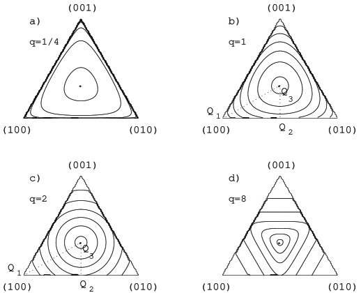
Figure 1. Iso-entropy curves in the space of probability distributions with $N=3$. The generalized Rényi entropy is constant along the curves plotted for (a) $q=1/4$, (b) $q=1$ (Shannon entropy), (c) $q=2$ (Euclidean circles–distance $D_{2}$), and (d) $q=8$. Dotted lines form the triangle $\triangle(Q_{1},Q_{2},Q_{3})$.

Superimposing some of the above pictures on one graph allows one to understand further relations between the Rényi entropies. The generalized entropies are correlated; e.g. for the distributions $Q_{k}$ the entropies are equal to $\ln k$ independently of the value of $q$.

The problem, which values the entropy $H_{q}$ may admit, provided $H_{s}$ is given, has been solved by Harremoës and Topsøe [15]. For any distribution $P\in{\mathbb{R}}^{N}$ they proved a simple (but not very sharp) upper bound on $H_{1}$ by $H_{2}$,

(16) $$H_{2}({\vec{x}})\leq H_{1}({\vec{x}})\leq\ln N+1/N-\exp(-H_{2}({\vec{x}}))$$

where the lower bound is a special case of (9). Moreover, they showed that the set $\Delta_{q,s}$ of possible probability distributions plotted in the plane $H_{q}$ versus $H_{s}$ is not convex (see Fig. 2), and its boundaries are formed of arcs corresponding to the interpolating probability distributions

(17) $$Q_{k,l}(a):=aQ_{k}+(1-a)Q_{l}\qquad{\rm with}\qquad a\in[0,1].$$

More precisely, for any probability distribution $P$ consisting of $N$ components and arbitrary $s>q>0$ the following bounds hold [15]

(18) $$H_{q}(Q_{k-1,k}(a))\leq H_{q}(P)\leq H_{q}(Q_{1,N}(a)),$$

where $a$ is a function of the known value of $H_{s}(P)$ and the natural number $k$ is selected by the inequality $\ln(k-1)\leq H_{s}(P)\leq\ln k$.

The above results, crucial for the main body of this work, are easy to understand. Let us discuss the simplest nontrivial case with $N=3$. The two dimensional simplex of probability distributions may be divided into $6$ identical parts, equivalent to the triangle $\triangle(Q_{1},Q_{2},Q_{3})$, as shown in Fig. 1c. Three sides of the triangle are formed of the interpolating distributions $Q_{1,2}$, $Q_{1,3}$ and $Q_{2,3}$ and these distinguished probabability distributions are extreme in a sense that they lead to the bounds (18). The bounds between $H_{1}$ and $H_{2}$ for $N=3$ are presented in Fig. 2a. To obtain them it is sufficient to travel along the sides of the triangle $\triangle(Q_{1},Q_{2},Q_{3})$, computing $H_{1}$ and $H_{2}$ at each point and to plot the data obtained in the plane $H_{1}$ versus $H_{2}$.

More formally, the upper boundary of the set $\Delta_{q,s}$ consist of one arc derived from the family of distributions $Q_{1,N}(a)$; for any value of $a$ we compute $H_{s}(a)$, invert it to obtain $a(H_{s})$ and plot $H_{q}(a(H_{s}))$. In the case $N=3$ the upper bounds plotted in Fig. 2a, c and e arise from the hypotenuse $Q_{1},Q_{3}$ of the triangle $\triangle(Q_{1},Q_{2},Q_{3})$ from Fig. 1.b and c.

In the similar way the lower bound may be derived from the distributions $Q_{k,k+1}(a)$ for $k=1,...N-1$. It consists of $(N-1)$ arcs forming an cascade $H_{q}(Q_{1,2}(a))\smile H_{q}(Q_{2,3}(a))\smile\cdots\smile H_{q}(Q_{N-1,N}(a))$. Note that the distributions $Q_{k}$ are represented in each plot by the points $(\ln k,\ln k)$, which connect the neighbouring arcs. For $N=3$ the lower bound consists of two arcs, corresponding to the adjacent sides $Q_{1},Q_{2}$ and $Q_{2},Q_{3}$ of $\triangle(Q_{1},Q_{2},Q_{3})$.

The shape of the set $\Delta_{q,s}$ requires a comment. The $N-1$ dimensional simplex – the set of all $N$–points probability distributions is convex and any of its projections onto a plane forms a convex set. However, its image at the plane $H_{q}$ versus $H_{s}$ needs not to be convex, since the transformations $H_{q}({\vec{x}})$ and $H_{s}({\vec{x}})$ are nonlinear. The boundaries of $\Delta_{q,s}$ are obtained as the image of an appropriately chosen path on the boundary of the simplex. In the case considered it is the path $Q_{1}\to Q_{2}\to\cdots\to Q_{N}\to Q_{1}$, independently of the values of $q$ and $s$. Observe that the general structure of the set $\Delta_{q,s}$ does not depend on $s$. However, the larger difference $s-q$, the larger area of the set: the less information on $H_{q}$ is provided by $H_{s}$.

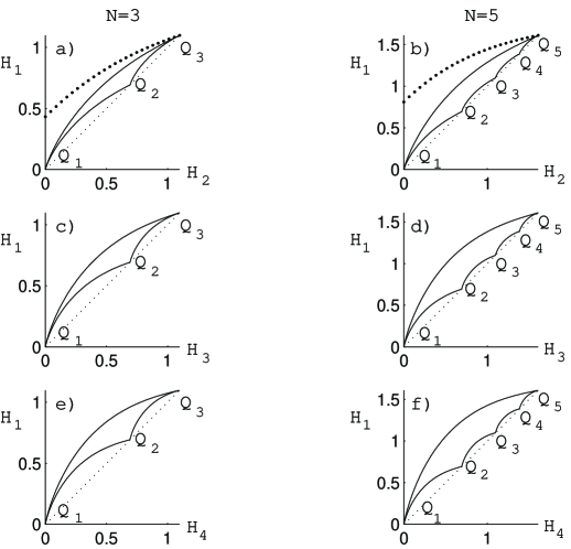
Figure 2. The set of all possible discrete distributions for $N=3$ and $N=5$ at the Rényi entropies plane $H_{1}$ and $H_{q}$: $q=2$ (a,b); $q=3$ (c,d) and $q=4$ (e,f). Thin dotted lines in each panel represent the monotonicity lower bounds (9) while bold dotted curves in panel (a) and (b) denote upper bound (16).

Let us emphasize in this point that results presented in [15] do not close the issue of finding bounds and relations between different entropies. Results analogous to (18) for a more general class of entropy functions were recently obtained by Berry and Sanders [17]. A more precise lower bound for Shannon entropy, quadaratic in terms of index of coincidence (purity) was found by Topsøe [18].

4. $N$–dependent bounds for Shannon entropy

4.1. Bounds based on $H_{2}$ and the length $N$ of the probability vector

Results (18) allow us to obtain bounds for a value of the entropy $H_{q}$, provided the value $H_{s}$ is known. Let us first assume that the entropy $H_{2}$ is known and we want to extract some information on $H_{1}$. We start computing the Rényi entropy of order two,

(19) $$H_{2}(Q_{1,N}(a))=-\ln\Bigl{[}\frac{(1+(N-1)a)^{2}}{N^{2}}+(N-1)\frac{(1-a)^{2}}{N^{2}}\Bigr{]}\$$

and invert it to obtain

(20) $$a=\sqrt{\frac{N\exp(-H_{2})-1}{N-1}}.$$

In this way we receive sharp upper bounds for $q\in(0,2)$

(21) $$H_{q}(P)\leq\frac{1}{1-q}\ln\Bigl{[}\Bigl{(}\frac{1+(N-1)a}{N}\Bigr{)}^{q}+(N-1)\Bigl{(}\frac{1-a}{N}\Bigr{)}^{q}\Bigr{]},$$

which for $q\to 1$ reduces to

(22) $$H_{1}(P)\leq H_{12}^{u}:=(1-N)\frac{1-a}{N}\ln\frac{1-a}{N}-\frac{1+a(N-1)}{N}\ln\frac{1+a(N-1)}{N}\ ,$$

with $a$ given by (20).

To obtain analogous lower bound we find $k$ such that $\ln(k-1)\leq H_{2}\leq\ln k$ and compute $H_{2}(Q_{k-1,k}(a))$. Also this relation may be easily inverted providing $a={\sqrt{k(k-1)\exp(-H_{2})+1-k}}$. Thus we arrive at a lower bound for the Rényi entropy

(23) $$H_{q}(P)\geq\frac{1}{1-q}\ln\Bigl{[}(k-1)z^{q}+y^{q}\Bigl{]}\ ,$$

and in particular case, for the Shannon entropy

(24) $$H_{1}(P)\geq H_{12}^{d}:=(1-k)z\ln z-y\ln y\ ,$$

with $z=(k+a-1)/(k^{2}-k)$ and $y=(1-a)/k$.

4.2. Bounds based on $H_{3}$ and $N$

Let us now assume, we know the value of the Rényi entropy $H_{3}$. As in (19) we compute $H_{3}(Q_{1,N}(a))$, and invert it finding $a\in[0,1]$ as the largest (real) root of the polynomial

(25) $$W_{u}(a)=a^{3}+a^{2}\frac{3}{N-2}-\frac{N^{2}\exp(-2H_{3})-1}{(N-1)(N-2)}=0.$$

Then the upper bound valid for $q\in(0,3)$ is given by the same formula (21) with $a$ given by the root of (25) instead of (20). For $q\to 1$ one obtains then the upper bound for the Shannon entropy

(26) $$H_{1}(P)\leq H_{13}^{u}:=(1-N)\frac{1-a}{N}\ln\frac{1-a}{N}-\frac{1+a(N-1)}{N}\ln\frac{1+a(N-1)}{N}\ ,$$

with $a$ determined by (25).

To get the lower bound we look for $k^{\prime}$ such that $\ln(k^{\prime}-1)\leq H_{3}\leq\ln k^{\prime}$. The relation $H_{3}(Q_{k^{\prime}-1,k^{\prime}}(a))$ may be inverted explicitly for $k^{\prime}=2$ providing $a={\sqrt{[4\exp(-2H_{3})-1]/3}}$. For $k^{\prime}>2$ $a$ is given by the only root of the polynomial

(27) $$W_{d}(a)=a^{3}+a^{2}\frac{3(k^{\prime}-1)}{2-k^{\prime}}+\frac{(k^{\prime}-1)^{2}}{2-k^{\prime}}[1-{k^{\prime}}^{2}\exp(-2H_{3})]=0.$$

in the interval $[0,1]$. The lower bound for the Rényi entropies has the same form as (23) and gives for the Shannon entropy

(28) $$H_{1}(P)\geq H_{13}^{d}:=(1-k^{\prime})z^{\prime}\ln z^{\prime}-y^{\prime}\ln y^{\prime}$$

with $z^{\prime}=(k^{\prime}+a-1)/(k^{\prime}(k^{\prime}-1))$ and $y^{\prime}=(1-a)/k^{\prime}$.

5. Combined extrapolation

In previous section we obtained two upper bounds for the Shannon entropy: (23) stemming from the Rényi entropy $H_{2}$, and (12) obtained from $H_{3}$. The latter is in general a worse one, but it allows for a linear extrapolation, which gives

(29) $$H_{up}({\vec{x}}):=2H^{u}_{12}({\vec{x}})-H^{u}_{13}({\vec{x}}).$$

Our numerical results allow us to advance the following

Conjecture.

For any probability distribution ${\vec{x}}$ the bound

(30) $$H_{1}({\vec{x}})\leq H_{up}({\vec{x}})$$

holds.

In the same way one may try to extrapolate lower bounds defining $H_{d}({\vec{x}}):=2H^{d}_{12}({\vec{x}})-H^{d}_{13}({\vec{x}})$. For certain probability vectors this quantity may give a useful approximation for the Shannon entropy. Interestingly, a relation analogous to (30), $H_{1}({\vec{x}})\geq H_{d}({\vec{x}})$ is not true: it is violated e.g. if $k\neq k^{\prime}$.

Making use of the rigorous bound (12) and the conjecture (30) we may suggest to estimate the unknown value of the Shannon entropy by the mean value

(31) $$H_{*}^{\prime}({\vec{x}}):=\frac{1}{2}[H_{up}({\vec{x}})+H_{d23}({\vec{x}})]=H^{u}_{12}({\vec{x}})+H_{2}(\vec{x})-\frac{1}{2}[H^{u}_{13}({\vec{x}})+H_{3}(\vec{x})],$$

which is obtained by combined methods based as well on the lower as well as on the upper bounds. Observe that this explicitly computable quantity involves only Rényi entropies $H_{2}$ and $H_{3}$ and the dimension $N$. This estimation may be improved noting that the rigorous lower bounds (12) and (24) are not equivalent. Since for some distributions the latter bound gives better (higher) results, we may improve (31) writing

(32) $$H_{*}({\vec{x}}):=\frac{1}{2}H_{u}({\vec{x}})+\frac{1}{2}{\rm max}\{H_{d23}({\vec{x}}),H^{d}_{12}({\vec{x}})\}.$$

If the value of the zero-entropy, $H_{0}$, is known, one may replace the upper bound $H_{u}({\vec{x}})$ used above by the minimum, ${\rm min}\{H_{u0}({\vec{x}}),H_{up}({\vec{x}})\}$.

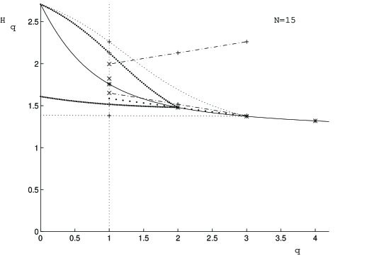
Figure 3. Rényi entropies $H_{q}$ for a random probability distribution of size $N=15$ (solid line). Dense dotted curves represent $H_{2}$ bounds: upper (21) and lower (23), while faint dotted curve denote analogous bounds based on $H_{3}$. Straight dashed–dotted lines show lower (12) and upper (29) extrapolations. The exact value of $H_{1}$ is denoted by $(*)$, while the estimation (32) by the middle $(\times)$.

Figure 3 shows the bounds and the estimations described above for a randomly chosen probability distributions with $N=15$ components. The overall quality of the proposed estimations for the Shannon entropy may be judged from Fig. 4, which shows the histogram of the deviations $\delta_{1}=H_{*}-H_{1}$ and $\delta_{2}=H_{d}-H_{1}$ for a sample of $10^{4}$ probability vectors generated randomly according to the statistical (Fisher–Rao) measure on the $N-1$ dimensional simplex [19]. This measure has a simple geometric interpretation: is suffices to consider a unit vector ${\vec{t}}$ distributed uniformly on the sphere $S^{N-1}$, and to define the probability vector ${\vec{x}}=\{t_{1}^{2},...,t_{N}^{2}\}$. Numerical results obtained in this way allow us to conclude that the proposed estimation (32) provides a useful all-purpose approximation of the Shannon entropy. Note that the precision of this approximation decreases with the length $N$ of the probability vector.

To judge about possible application of the estimate $H_{*}$ in the analysis of physical data, one should perform analogous numerical simulations with random vectors ${\vec{x}}$ generated according to a specific probability distribution adjusted to a given physical problem.

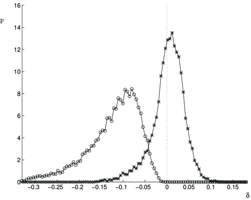
Figure 4. Histogram of deviations of the extrapolations form the real value of the Shannon entropy $H_{1}$: $(*)$ denotes the probability density of error $\delta_{1}=H_{*}-H_{1}$ of the estimation (32), while $(o)$ denotes results for the error $\delta_{2}=H_{d}-H_{1}$ of the lower bound (12) for a sample of $10^{4}$ random probability vectors of size $N=10$.

6. Concluding Remarks

In this work we considered the problem of finding the bounds and extrapolations for the Shannon (entropy), provided some of the Renyi entropies are known. In general, generalized entropies of integer order $q=2$ and $q=3$ are easiest to calculate, and they are sufficient to obtain bounds (10) and (12) for the Shannon entropy. The quality of the bound may be improved if the length $N$ of the probability vector is known. Then an explicit extrapolation (32) allows us to estimate the actual value of the entropy $H$.

Note that the bounds and extrapolations discussed may be easily rewritten in terms of a non-extensive entropy

(33) $$S_{q}(\vec{x}):=\frac{1}{1-q}\Bigl{[}\sum_{i=1}^{n}x_{i}^{q}-1\Bigr{]}\$$

used by Havrda and Charvat [20] and Daroczy [21], which became often used in statistical physics after the seminal work of Tsallis [22]. In particular, the linear entropy $L$ is just the nonextensive entropy of order two, $L({\vec{x}})=S_{2}(\vec{x})$, and the bounds between $H_{q}$ and $H_{1}$ imply analogous relations between $S_{q}$ and $H_{1}$. In fact the plot presented in [13] shows bounds between von Neumann entropy and the linear entropy and they follow directly from relation (18) proven in [15].

The issue of comparing the Rényi entropies $H_{0}$, $H_{1}$ and $H_{2}$ is closely related to the problem of describing the degree of chaos of an analyzed classical dynamical system by the topological entropy $K_{0}$, the Kolmogorov–Sinai (metric) entropy $K_{1}$ and the correlation entropy $K_{2}$. These dynamical entropies are defined as the rate of the increase of the Rényi entropies in time [16], but since the length of the probability vector is not finite the $N$–dependent bounds discussed in this work are not applicable. The same concerns comparison of generalized fractal dimensions $D_{q}$ of fractal measures: the box–counting dimension $D_{0}$, the information dimension $D_{1}$ and the correlation dimension $D_{2}$, which also form a non–increasing function of the Rényi parameter $q$ [16], are defined by the limit $N\to\infty$.

The generalized entropies may also be used to characterize localization properties of continuous probability distributions. For instance, any pure quantum state may be represented in the phase space by the Husimi distribution. Its localization can be measured by the Wehrl entropy defined as the continuous (Boltzmann–Gibbs) entropy of the Husimi distribution [23]. In an analogous way one may define generalized Rényi–Wehrl entropies [24, 11], and above results may be used to obtain similar bounds for the Wehrl entropy.

It is a pleasure to thank P. Harremoës and F. Topsøe for explaining us their results prior to publication and several fruitful comments. I am also thankful to I. Bengtsson, A.Białas, A. Ostruszka, F. Mintert, W. Munro and W. Słomczyński for inspiring discussions and D. Berry, B. Sanders and I. Varga for helpful correspondence. Financial support by Komitet Badań Naukowych in Warsaw under the grant 2P03B-072 19 and by a research grant of the Volkswagen Stiftung is gratefully acknowledged.

7. Corrigendum    –   February 17, 2005

Eq. (8) implies that $(1-q)H_{q}$ is a convex function of $q$. However, it does not imply that the Rényi entropy $H_{q}$ is a convex function of $q$. For instance, the Rényi entropy for a $N=20$ probability vector $P=\frac{1}{100}(43,3,\dots,3)$ is not a convex function of $q$. I am deeply obliged to Christian Schaffner for drawing my attention to this fact.

Therefore, equations (10), (11), and (12) are not satisfied and conjecture (30) cannot hold. Furthermore, equations (13), (31), (32) may only be used to extrapolate the unknown value of the Shannon entropy, from the available data on $H_{2}$ and $H_{3}$.

On the other hand, we would like to mention that the lack of convexity of $H_{q}$ in $q$ does not influence the bounds between particular values of the Rényi entropy presented in sections 3 and 4 of the present paper.

References

- [1] C. Shannon, Mathematical theory of communication, Bell System Tech. J. 27, 379 (1948)
- [2] A. I. Khinchin, Mathematical foundations of information theory, Dover, 1957,
- [3] A. Rényi, On measures of entropy and information, in. Proc. Fourth. Berkeley Symp. Math. Stat. Prob. 1960, Vol. I, p.547, (University of California Press, Berkeley, 1961).
- [4] J. N. Kapur, Measures of Information and Their Applications (John Wiley & Sons, New York, 1994).
- [5] C. Arndt. Information Measures: Information and its Description in Science and Engineering (Springer, Berlin 2001).
- [6] P. Horodecki and A. Ekert, Direct detection of quantum entanglement, Phys. Rev. Lett. 89, 127902 (2002).
- [7] C. M. Alves, P. Horodecki, D. K. L. Oi, L. C. Kwek, and A. K. Ekert, Direct estimation of functionals of density operators by local operations and classical communication, preprint quant-ph/0304123
- [8] A. Białas and W. Czyż, Renyi Entropies in Multiparticle Production, Acta Phys. Pol. B 31, 2803 (2000).
- [9] A. Białas, W. Czyż and A. Ostruszka, Renyi entropies in particle cascades, Acta Phys. Pol. B 34, 69 (2003).
- [10] J. Pipek and I. Varga, Universal scheme for the spacial–localization properties of one–particle states in finite –dimensional systems, Phys. Rev. A 46, 3148 (1992).
- [11] I. Varga and J. Pipek, On Rényi entropies characterizing the shape and the extension of the phase space representation of quantum wave functions in disordered systems, arXiv preprint cond-mat/0204041 (2002).
- [12] K. Życzkowski, I. Bengtsson, Relativity of pure states entanglement, Ann. Phys. (N.Y.) 295, 115-135 (2002)
- [13] T.-C. Wei, K. Nemoto, P.M. Goldbart, P.G. Kwiat, W.J. Munro and F. Verstraete, Maximal entanglement versus entropy for mixed quantum states, Phys. Rev. A 67, 022110 (2003)
- [14] F. Topsøe, Some inequalities for information divergence and Related measures of discrimination IEEE Trans. Inform. Theory 46, 1602 (2000).
- [15] P. Harremoës and F. Topsøe, Inequalities between Entropy and Index of Coincidence derived from Information Diagrams, IEEE Trans. Inform. Theory 47, 2944-2960 (2001)
- [16] C. Beck and F. Schlögl, Thermodynamics of chaotic systems, (Cambridge University Press, Cambridge, 1993).
- [17] D. W. Berry and B. C. Sanders, Bounds on entropy, preprint arXiv quant-ph/0305059, (2003)
- [18] F. Topsøe, Entropy and Index of Coincidence, lower bounds, preprint, Copenhagen, 2003
- [19] R. A. Fisher, Theory of Statistical Estimation Proc. Cambridge Philos. Soc. 22, 700 (1925).
- [20] J. Havrda and F. Charvat, Quantification methods of classification Processes: Concept of structural –Entropy, Kybernetica 3, 30 (1967)
- [21] Z. Daroczy, Inf. Control 16, 36 (1970)
- [22] C. Tsallis, Possible generalization of Boltzmann–Gibs statistics, J. Stat. Phys. 52, 479 (1988)
- [23] A. Wehrl, General properties of entropy, Rev. Mod. Phys. 50, 221 (1978)
- [24] S. Gnutzmann and K. Życzkowski, Renyi-Wehrl entropies as measures of localization in phase space, J. Phys. A 34, 10123-10139 (2001).