Classical trajectories and quantum tunneling

Abstract

The problem of inter-band tunneling in a semiconductor (Zener breakdown) in a nonstationary and homogeneous electric field is solved exactly. Using the exact analytical solution, the approximation based on classical trajectories is studied. A new mechanism of enhanced tunneling through static non-one-dimensional barriers is proposed in addition to well known normal tunneling solely described by a trajectory in imaginary time. Under certain conditions on the barrier shape and the particle energy, the probability of enhanced tunneling is not exponentially small even for non-transparent barriers, in contrast to the case of normal tunneling.

I INTRODUCTION

A control of processes of quantum tunneling through potential barriers by external signals is a part of the field called quantum control which is actively developed now, see, for example, Ref. [1] and references therein. Excitation of molecules, when one should excite only particular chemical bonds [2, 3, 4], formation of programmable atomic wave packets [5], a control of electron states in heterostructures [6, 7], and a control of photocurrent in semiconductors [8], are typical examples of control by laser pulses. A control of quantum tunneling through potential barriers is also a matter of interest, since tunneling is a part of many processes in nature. The computation of probability for a classically forbidden region has a certain peculiarity from the mathematical stand point: there necessarily arises here the concept of motion in imaginary time or along a complex trajectory [9, 31, 34]. The famous semiclassical approach of Wentzel, Kramers, and Brillouin (WKB) [9] for tunneling probability can be easily (in the case of a static potential) reformulated in terms of classical trajectories in complex time as a simple change of variables. The method of complex trajectories can also be applicable to a nonstationary case [12, 13] which is not trivial. The method has been further developed in papers [14, 15, 16, 17, 18], when singularities of the trajectories in the complex plane were accounted for an arbitrary potential barrier (see also [19]). Recent achievements in the semiclassical theory are present in Refs.[20, 21, 22, 23, 24].

Let us focus on the main aspects of tunneling under nonstationary conditions. When the electric field ${\cal E}\cos\Omega t$ acts on a tunneling particle of the initial energy $E$, it can absorb the quantum $\hbar\Omega$ (with the probability proportional to the small parameter ${\cal E}^{2}$) and tunnel after that in a more transparent part of the barrier with the higher energy $E+\hbar\Omega$. The pay in the absorption probability may be compensated by the probability gain in tunneling. In this case the system tends to absorb further quanta to increase the total probability of passing the barrier. This mechanism of barrier penetration is called photon-assisted tunneling. If $\hbar\Omega$ is not big, the process of tunneling, with the simultaneous multi quanta absorption, can be described in a semiclassical way by the method of classical trajectories in the complex time [14, 15, 16, 17, 18]. When a tunneling particle of the energy $E$ is acted by a short-time pulse, the tunneling probability is associated with the particle density carrying away in the outgoing wave packet. The particle energy after escape is $E+\delta E$, where the energy gain $\delta E=N\hbar\omega$, should be extremized with respect to the number of absorbed quanta $N$ and the energy $\hbar\omega$ of each quantum [25, 26]. This mechanism relates to semiclassical method for nonstationary potentials.

The semiclassical method in quantum mechanics is very elegant and constructive. On the other hand, this method is based on the delicate mathematical issue called Stokes phenomenon when a solution is not expected to appear but it appears [27]. This makes a use of the semiclassical method to be not trivial even in the case of a static potential. In this situation the role of exactly solvable problems in quantum mechanics is very important. For example, in the problem of reflection of a particle from certain static potentials one can follow in details a formation of a semiclassical solution from the exact one [9]. Is it possible to find an exactly solvable problem for a nonstationary potential (excepting not interesting parabolic one, where the effect is trivial [17, 18]) to see how the exact solution is reduced to complex classical trajectories under semiclassical conditions? An exactly solvable problems would be extremely useful since the method of classical trajectories in nonstationary problems is still challenged and an exact analytical solution would place classical trajectories in the rank of mathematical theorem.

Such exactly solvable nonstationary problem exists. This is an inter-band tunneling (Zener breakdown) in a semiconductor [28] in a nonstationary electric field which is a constant in space. The latter condition makes the problem to be exactly solvable since in the momentum representation the Schrödinger equation is reduced to the first order which can be solved by the method of characteristics. In this paper it is studied how the exact solution turns over into one corresponding to classical trajectories and under which conditions this is possible. The goal of the paper is not to investigate Zener effect in real semiconductors but to use this situation to mathematically justify the method of classical trajectories.

Another issue of this paper is that a new mechanism of enhanced tunneling through static non-one-dimensional barriers is proposed in addition to well known normal tunneling solely described by a trajectory in imaginary time. As shown in the paper, under certain conditions on the barrier shape and the particle energy, the probability of enhanced tunneling is not exponentially small even for non-transparent barriers, in contrast to the case of normal tunneling.

II PHOTON-ASSISTED TUNNELING

A penetration of a particle through a potential barrier is forbidden in classical mechanics. Only due to quantum effects the probability of passing across a barrier becomes finite and it can be calculated on the basis of WKB approach, which is also called the semiclassical theory. The transition probability through the barrier, shown in Fig. 1, is

$$W\sim\exp\left[-A_{0}(E)\right]$$ (1)

where

$$A_{0}(E)=\frac{2}{\hbar}\int dx\sqrt{2m\left[V(x)-E\right]}$$ (2)

is the classical action measured in units of $\hbar$. The integration goes under the barrier between two classical turning points where $V(x)=E$. One can use the general estimate $A_{0}\sim V/\hbar\omega$, where $V$ is the barrier height and $\omega$ is the frequency of classical oscillations in the potential well. A semiclassical barrier relates to a big value $V/\hbar\omega\gg 1$.

What happens when the static potential barrier $V(x)$ is acted by a weak nonstationary electric field ${\cal E}(t)$? In this case there are two possibilities for barrier penetration: (i) the conventional tunneling, which is not affected by ${\cal E}(t)$, shown by the dashed line in Fig. 2(a), and (ii) an absorption of the quantum $\hbar\Omega$ of the field ${\cal E}(t)$ and subsequent tunneling with the new energy $E+\hbar\Omega$. The latter process is called photon-assisted tunneling. The total probability of penetration across the barrier can be schematically written as a sum of two probabilities

$$W\sim\exp\left(-\frac{V}{\hbar\omega}\right)+\left(\frac{a\hskip 1.42271pt{\cal E}_{\Omega}}{\hbar}\right)^{2}\exp\left(-\frac{V-\hbar\Omega}{\hbar\omega}\right)$$ (3)

where ${\cal E}_{\Omega}$ is the Fourier component of the field ${\cal E}(t)$ and the length $a$ is a typical barrier extension in space. The second term in Eq. (3) relates to photon-assisted tunneling and it is a product of probabilities of two quantum mechanical processes: absorption of the quantum $\hbar\Omega$ and tunneling through the reduced barrier $V-\hbar\Omega$. Since in quantum mechanics one should add amplitudes but not probabilities, Eq. (3) is rather schematic and serves for general illustration only. For example, the accurate perturbation theory starts with a linear ${\cal E}$-term. When the frequency is high $\Omega>\omega$, the second dominates at sufficiently small nonstationary field $(a{\cal E}_{\Omega}/\hbar)^{2}>\exp(-\Omega/\omega)$. This is a feature of tunneling processes since, normally, a nonstationary field dominates at bigger amplitudes $(a{\cal E}_{\Omega}/\hbar)^{2}>1$. When the second term in Eq. (3) exceeds the first one, further orders of perturbation theory should be accounted which correspond to the multiple absorption, shown in Fig. 2(b).

Let us specify a shape of a field pulse in the form

$${\cal E}(t)=\frac{{\cal E}}{\left(1+t^{2}/\theta^{2}\right)^{3}}$$ (4)

with the Fourier component ${\cal E}_{\Omega}\sim{\cal E}\theta\exp(-\theta|\Omega|)$. In this case, in addition to the almost steady flux from the barrier, an outgoing wave packet (of the maximum amplitude $\sqrt{W}$) is created which carries away a certain particle density. The probability of the transition through the process of absorption of $N$ quanta and subsequent tunneling with the higher energy $E+N\hbar\Omega$, shown in Fig. 2(b), can be estimated as

$$w\sim\left(\frac{a{\cal E}_{\Omega}}{\hbar}\right)^{2N}\exp\left[-A_{0}(E+N\hbar\Omega)\right]=\left(\frac{\pi}{\hbar}\hskip 1.42271pt\theta a{\cal E}\right)^{2N}\exp(-A)$$ (5)

where

$$A=\frac{2\theta}{\hbar}\hskip 2.84544pt\delta E+A_{0}(E+\delta E)$$ (6)

Here the total energy transfer $\delta E=N\hbar\Omega$ is introduced ($\Omega>0$). The maximum squared amplitude $W$ of the outgoing packet is associated with a maximum value of $w$ and is determined by the extreme $\delta E$ to get a minimum of $A$. This results in the condition $\partial A(E+\delta E)/\partial\delta E=0$. An existence of such a minimum is possible if growing up of small $\delta E$ reduces $A$, that is, under the condition $2\theta<\hbar\mid\partial A_{0}(E)\partial E\mid$ of sufficiently short pulses. In other words, sufficiently short and not very small pulses (however, still much smaller than the static barrier field) strongly enhance tunneling by photon assistance.

In principal, this type of treatment of nonstationary tunneling is reasonable since a maximum of the outgoing packet should relate to some extreme condition. Nevertheless, the approach (5) is schematic since a quantum interference between absorption and tunneling is neglected. What is a “scientific” way to account precisely a nonstationary field in tunneling? We go towards this in III.

III TRAJECTORIES IN IMAGINARY TIME

According to Feynman [29], when the phase of a wave function is big, it can be expressed through classical trajectories of the particle. But in our case there are no conventional trajectories since a classical motion is forbidden under a barrier. Suppose a classical particle to move in the region to the right of the classical turning point $x_{T}$ in Fig. 1 and to reach this point at $t=0$. Then, close to the point $x_{T}$, $x(t)=x_{T}+ct^{2}$ ($c>0$) and there is no a barrier penetration as at all times $x(t)>x_{T}$. Nevertheless, if $t$ is formally imaginary, $t=i\tau$, the penetration becomes possible since $x(i\tau)=x_{T}-c\tau^{2}$ is less then $x_{T}$. Therefore, one can use classical trajectories in imaginary time to apply Feynman’s method to tunneling. In the absence of a nonstationary field a classical trajectory satisfies Newton’s equation in imaginary time

$$m\hskip 2.84544pt\frac{\partial^{2}x}{\partial\tau^{2}}=\frac{\partial V(x)}{\partial x}$$ (7)

where $V(x)$ is the static barrier in Fig. 1. The classical turning point $x_{T}$ in Fig. 1 is reached at $\tau=0$ with the initial condition $\partial x/\partial\tau=0$. The classical trajectory $x=x(\tau)$ can be considered as a change of variables $x\rightarrow\tau$ in the WKB exponent (2) when it becomes of the form

$$A_{0}=\frac{2}{\hbar}\int d\tau\left[\frac{m}{2}\left(\frac{\partial x}{\partial\tau}\right)^{2}+V(x)-E\right]$$ (8)

So, in the absence of a non-stationary field, use of classical trajectories in imaginary time is obvious and it is simply reduced to a change of variable.

Is it possible to extend the method of classical trajectories in tunneling to a non-stationary case?

Suppose some pulse of an external field, for example (4), acts on a tunneling particle. At the point $x_{T}$, besides an almost constant background, there is a wave packet of the outgoing particles shown in Fig. 3. If the method of classical trajectories is applicable, the maximum of the squared amplitude of the outgoing packet

$$W\sim\exp(-A)$$ (9)

should correspond, with the exponential accuracy, to the classical action

$$A=\frac{2}{\hbar}\int^{\tau_{0}}_{0}d\tau\left[\frac{m}{2}\left(\frac{\partial x}{\partial\tau}\right)^{2}+V(x)-x{\cal E}(i\tau)-E\right]$$ (10)

since a classical trajectory relates to an extreme value of the action. The classical trajectory should satisfy Newton’s equation

$$m\hskip 2.84544pt\frac{\partial^{2}x}{\partial\tau^{2}}-\frac{\partial V(x)}{\partial x}=-{\cal E}(i\tau)$$ (11)

with the conditions

$$\frac{\partial x}{\partial\tau}\bigg{|}_{\tau=0}=0;\hskip 28.45274ptx(i\tau_{0})=0$$ (12)

We suppose the potential well to be narrow and localized close to $x=0$ as in Fig. 1. The under-barrier “time” $\tau_{0}$ is expressed through the particle energy $E$ in the well

$$E=\frac{m}{2}\left(\frac{\partial x}{\partial\tau}\right)^{2}_{\tau_{0}}+V(0)$$ (13)

which is weakly violated by a small non-stationary field. Certain semiclassical conditions (not extremely small and sufficiently slow varying ${\cal E}(t)$) should be fulfilled.

Eqs. (9-13) constitute the method of classical trajectories in tunneling under non-stationary conditions. This method relates to calculation solely of the maximum in time $W_{max}$ of the probability $W(t)$ of outgoing particles. In contrast to a static barrier, the method of classical trajectories is not trivial in application to a nonstationary case. This can be seen from that the non-stationary field of the type ${\cal E}\cos\Omega t$ in imaginary time becomes proportional to $\cosh\Omega\tau$ and may be very big. The same relates to the field (4) which is singular in imaginary time. This means, formally, that arbitrary weak amplitude ${\cal E}$ of a nonstationary field may produce a big effect. The arguments in II also show an increase of an effective ${\cal E}$ in tunneling, but it is clear physically that an effect of an extremely small nonstationary field is negligible and the method of classical trajectories should not work in this case. As one can see, the method of classical trajectories is delicate and requires an accurate justification.

In the papers [25, 26] for the certain particular potential well and nonstationary pulses the wave function has been found in the form of expansion with respect to powers of $\hbar$

$$\psi(x,t)=\left[a(x,t)+\hbar b(x,t)+...\right]\exp\left[\frac{i}{\hbar}\hskip 2.84544ptS(x,t)\right]$$ (14)

where $S$ is the classical action. The semiclassical formalism, developed in [25, 26], confirms the method of classical trajectories and coincides with the general scheme (9-13). Nevertheless, it would be extremely instructive to find any exactly solvable case of tunneling under nonstationary conditions in order to see how the method of classical trajectories follows not from a semiclassical formalism but from an exact mathematical solution. In IV this program is completed.

IV EXACT SOLUTION OF A TUNNELING PROBLEM UNDER NONSTATIONARY CONDITIONS

Let us consider an one dimensional two band semiconductor in an external homogeneous electric field ${\cal E}_{0}+{\cal E}(t)$, where ${\cal E}_{0}$ is the static component. The Schrödinger equation has the form

$$i\hbar\hskip 2.84544pt\frac{\partial\psi}{\partial t}=\frac{\varepsilon_{g}}{2}\hskip 2.84544pt\sqrt{1+\left(\frac{2c}{\varepsilon_{g}}\hskip 2.84544pt\hat{p}\right)^{2}}\hskip 5.69046pt\psi-\left[{\cal E}_{0}+{\cal E}(t)\right]\psi$$ (15)

where $\hat{p}=-i\hbar\partial/\partial x$, $\varepsilon_{g}$ is the energy gap, and $c$ is the velocity at big momentum. The square root in Eq. (15) may have two signs according to two energy bands. In a static electric field ${\cal E}_{0}$ the inter-band quantum tunneling is possible which is called Zener breakdown [28]. The incident flux of particles from left to the right in Fig. 4 is mainly reflected back from the tilted energy gap but a small fraction penetrates the other band and goes to $+\infty$ with the probability [28]

$$W_{0}=\exp\left(-\frac{\pi\varepsilon_{g}t_{0}}{2\hbar}\right)$$ (16)

where $t_{0}=a/c$ and $2a=\varepsilon_{g}/{\cal E}_{0}$ is the tunneling length in Fig. 4. Eq. (16) holds under the semiclassical condition

$$\hbar\ll\varepsilon_{g}t_{0}$$ (17)

The peculiarity of this problem is that it can be solved exactly with a nonstationary field by making the Fourier transformation with respect to $x$. In the new variables, momentum $q$ and time $t$, the Schrödinger equation (15) is of the first order with respect to derivatives $\partial/\partial q$ and $\partial/\partial t$ and can be solved by the method of characteristics. If to measure the coordinate in units of $a$ and time in units of $t_{0}$, the solution of Eq. (15) has the form

$$\psi(x,t)=\int^{\infty}_{-\infty}\frac{dq}{2\pi}\exp\left\{\frac{i\varepsilon_{g}t_{0}}{2\hbar}\left[qx-F_{t}(q)\right]\right\}$$ (18)

where

$$F_{t}(q)=\int^{q}_{-\infty}duf_{t}(u,q);\hskip 28.45274ptf_{t}(u,q)=\sqrt{1+\left[u+\int^{u-q}_{0}dsh(s+t)\right]^{2}}$$ (19)

and $h(t)={\cal E}(t)/{\cal E}_{0}$. Below we consider the case when the nonstationary field is much less compared to the static value

$${\cal E}(t)\ll{\cal E}_{0}$$ (20)

If ${\cal E}(t)$ is an analytical function of $t$, $F_{t}(q)$ is an analytical function of the complex argument $q$ and it has only two branch points at $q=\pm i$. According to this, Eqs. (18-19) can be written through the complex paths

$$\psi(x,t)=\int_{C}\frac{dq}{2\pi}\exp\left\{\frac{i\varepsilon_{g}t_{0}}{2\hbar}\left[qx-F_{t}(q)\right]\right\};\hskip 28.45274ptF_{t}(q)=\int_{C{q}}duf_{t}(u,q)$$ (21)

where the contour $C$ on the complex plane of $q$ and the contour $C_{q}$ on the complex plane of $u$ are shown in Fig. 5. Two cuts are denoted in Fig. 5(a) by solid lines and the regular branch of the function $F_{t}(q)$ is chosen in order to get the limit

$$F_{t}(q)=-\int^{q}_{-\infty}du|f_{t}(u,q)|;\hskip 28.45274ptq\rightarrow-\infty$$ (22)

The integral (22) is divergent and has to be cut off at the lower limit by a big negative value which sets an irrelevant constant phase shift. Under the semiclassical condition (17) the $q$-integration in Eq. (21) goes mainly in the vicinity of the saddle point(s) determined by the equation

$$x=\frac{\partial}{\partial q}\hskip 2.84544ptF_{t}(q)$$ (23)

Suppose the nonstationary field ${\cal E}(t)\rightarrow 0$ at $t\rightarrow-\infty$ when the particle energy is zero and the particle goes to the tilted energy gap in Fig. 4 from the left. For $x$ to the left of the point $-a$ in Fig. 4 ($x<-1$ in the dimensionless units used) an influence of the nonstationary field under the condition (20) is small and two saddle points $q=\pm\sqrt{x^{2}-1}$ are shown in Fig. 6(a). They correspond to the incident and the reflected de Broglie waves. Since the tunneling probability is small, at $x<-1$ the wave function can be shown to have the form

$$\psi(x,t)\sim\cos\left(\frac{\varepsilon_{g}t_{0}}{4\hbar}x^{2}-\frac{\pi}{4}\right)$$ (24)

In the classically allowed regions, to the left and to the right of the tilted gap, the classical trajectory $x_{cl}(t)$ (the equation, it satisfies, is written below) is weakly violated by the non-stationary field under the condition (20)

$$x_{cl}(t)=\begin{cases}-\sqrt{1+t^{2}};&t<0\\ x_{exit}+\sqrt{1+t^{2}}-1;&t>0\end{cases}$$ (25)

excepting that $x_{exit}\neq 1$ now. The energy of the incident particle is zero and the energy after exit from the tilted gap conserves and equals $E_{exit}=(1-x_{exit})\varepsilon_{g}/2$.

For each $x$ and $t$ the saddle point condition (23) determines a certain $q$. In the absence of a nonstationary field the amplitude of the outgoing wave is almost stationary. Under action of a pulse there is an additional outgoing wave packet at $t>0$ which goes to the right and keeps the constant maximum amplitude (if to neglect small quantum effects of smearing) at the classical trajectory (25). We are interested to find this maximum amplitude of the outgoing packet since it defines, with the exponential accuracy, a total number of particles passing the barrier. With $x=x_{cl}(t)$ the saddle point condition (23) is satisfied by $q=t$ since $h(t)$ is small for real $t$. In order to reach the saddle point at positive $x$, one should deform the contour $C$ as shown in Fig. 6(b). This could be done with no problems since $F_{t}(q)$ has only the branch point at $q=i$ in the upper half plane. The main contribution to the $q$-integration over the bent contour $C$ comes from the saddle point, shown in Fig. 6(b). The saddle point condition (23) now reads

$$x_{exit}=1-2\int^{\tau_{0}}_{0}d\tau\hskip 2.84544pt\frac{\tau+\int^{\tau}_{0}d\tau_{1}h(i\tau_{1})}{\sqrt{1-\left[\tau+\int^{\tau}_{0}d\tau_{1}h(i\tau_{1})\right]^{2}}}\hskip 2.84544pth(i\tau)$$ (26)

The nonstationary field is supposed to be symmetric ${\cal E}(t)={\cal E}(-t)$, as the field (4), so that ${\cal E}(i\tau)$ is real. $\tau_{0}$ is a smallest positive root of the equation

$$\left[\tau_{0}+\int^{\tau_{0}}_{0}d\tau h(i\tau)\right]^{2}=1$$ (27)

and can be called the tunneling time. If to define the transition probability $W$ as a square of the ratio of the maximum amplitude of the outgoing packet and the amplitude of the incident wave, Eq. (18) gives with the exponential accuracy

$$W\sim\exp\left(-A\right)$$ (28)

where

$$A=\frac{2\varepsilon_{g}t_{0}}{\hbar}\int^{\tau_{0}}_{0}d\tau\sqrt{1-\left[\tau+\int^{\tau}_{0}d\tau_{1}h(i\tau_{1})\right]^{2}}$$ (29)

The action $A$ is collected due to the $q$-integration in the narrow vicinity of the right-hand-side saddle in Fig. 6(b) where $q$ is real and positive. For such $q$ the contour $C_{q}$ in Fig. 5(b) goes around the branch point $u=i\tau_{0}$ and leads to the relation (29). Without a non-stationary field Eqs. (28) and (29) give the static result (16).

Using of the above method of saddle point means that the length $\delta q\sim\sqrt{\hbar/\varepsilon_{g}t_{0}}$ of the steepest descent integration should be sufficiently short compared to the typical scale of the problem ($(\tau-\theta)/t_{0}$ in dimension units) which can be estimated from the relation $\int d\tau h(i\tau)\sim 1$. For the pulse (4) the condition reads

$$\frac{\hbar}{\varepsilon_{g}t_{0}}\ll\left(\frac{\theta}{t_{0}}\right)^{3}\frac{{\cal E}}{{\cal E}_{0}}$$ (30)

In presence of a nonstationary field, the semiclassical condition (17) should be supplemented by the additional semiclassical condition (30). According to it, the nonstationary field ${\cal E}$ and its duration $\theta$ should not be too small. Note, that under the semiclassical condition (30) the nonstationary amplitude ${\cal E}$ can be still smaller than the static field ${\cal E}_{0}$.

In Refs. [17, 18] the method of classical trajectories was developed for the present problem of inter-band tunneling in presence of a nonstationary field. According to this method, one has to minimize the classical action of a particle with the spectrum, as in (15,) and in a homogeneous electric field

$$S=\frac{\varepsilon_{g}t_{0}}{2}\int dt\left\{\sqrt{1-\left(\frac{\partial x}{\partial t}\right)^{2}}+x\left[1+h(t)\right]\right\}$$ (31)

to find a classical trajectory. It satisfies the equation

$$\frac{\partial x_{cl}(t)}{\partial t}=\frac{t+\int^{t}_{0}dsh(s)}{\sqrt{1+\left[t+\int^{t}_{0}dsh(s)\right]^{2}}}$$ (32)

The classical trajectory starts at $t=0$ at the point $x=x_{exit}$ in Fig. 4. At the “moment” $i\tau_{0}$ it reaches some point inside the gap where two branches merge and, turning on the opposite side of the cut, it comes at $t=0$ in the point $x=-a$. Within the formalism, developed in Refs. [17, 18], in order to obtain a tunneling probability, one should substitute the classical trajectory into the action (31) and to integrate over the branch point $i\tau_{0}$. This procedure leads to the result (29).

For the nonstationary pulse (4) under the condition (20), the tunneling time $\tau_{0}\simeq 1$ at $t_{0}<\theta$ and $\tau_{0}\simeq\theta/t_{0}$ at $\theta<t_{0}$. The action (29) becomes of the form

$$A=\frac{\varepsilon_{g}t_{0}}{\hbar}\begin{cases}\pi/2\hskip 2.84544pt;&t_{0}<\theta\\ \arcsin\left(\theta/t_{0}\right)+\left(\theta/t_{0}\right)\sqrt{1-\left(\theta/t_{0}\right)^{2}}\hskip 2.84544pt;&\theta<t_{0}\end{cases}$$ (33)

This expression weakly depends on ${\cal E}$ under the semiclassical condition (30) since the role of the nonstationary field (4), due to its singularity in imaginary time, is only to set the new tunneling time $\tau_{0}$. Obtained results for inter-band tunneling under nonstationary conditions may be interpreted as positive (positive energy transfer) photon-assisted tunneling shown in Fig. 4. In this problem cannot be such phenomenon as Euclidean resonance [26], associated with a negative energy transfer.

Analogously one can consider the monochromatic ${\cal E}\cos\Omega t$ [17, 18] and the Gaussian ${\cal E}\exp(-\Omega^{2}t^{2})$ nonstationary fields which become exponentially big in imaginary time and to establish how much they can grow within the formalism of classical trajectories.

One can conclude now, that for inter-band tunneling in a nonstationary field under semiclassical conditions the method of classical trajectories follows from the exact analytical solution. The bridge between exact theory and classical trajectories enables in problems of tunneling to treat a nonstationary field in complex time.

V A NEW ENHANCED TUNNELING THROUGH STATIC BARRIERS

Tunneling through one-dimensional static barrier is a well known problem described in almost every text book on quantum mechanics and the tunneling rate, with exponential accuracy, is given by WKB formulas (1) and (2). Tunneling through a two- or many-dimensional potential barrier was considered in a variety of publications [30, 31, 32, 33, 34, 35, 36, 37]. The condition $V(\vec{r})=E_{0}$, where $E_{0}$ is the total energy, determines certain surfaces in the coordinate space. For a two-dimensional case it is shown in Fig. 7. Tunneling probability from the classically allowed region $A$ to another such region $B$ is given by Eq. (1) where the exponent

$$A_{0}(A\rightarrow B)=\frac{2}{\hbar}\int^{\tau_{0}}_{0}d\tau\left[\frac{m}{2}\left(\frac{\partial\vec{r}}{\partial\tau}\right)^{2}+V(\vec{r})-E_{0}\right]$$ (34)

is expressed through the classical trajectory $\vec{r}(\tau)$ satisfying Newton’s equation in imaginary time

$$m\hskip 2.84544pt\frac{\partial^{2}\vec{r}}{\partial\tau^{2}}=\frac{\partial V(\vec{r})}{\partial\vec{r}}$$ (35)

The trajectory connects different surfaces, being perpendicular to them at the connected points, terminates at the border of $B$ at $t=0$, and starts at the border of $A$ at $t=i\tau_{0}$. The time $\tau_{0}$ is defined by the total energy $E_{0}$.

The above general scheme is applicable to a calculation of tunneling rate regardless of dimensionality of the problem (we do not consider a possibility of caustics between $A$ and $B$). Nevertheless, when the dimensionality is bigger than one, another way may exist to tunnel through a static potential barrier. This way differs from the normal scheme and may result in an enhanced tunneling rate. Any tunneling process obeys quantum mechanical rules: a tunneling particle at each point emits partial de Broglie waves which interfere and produce a final outgoing wave. This wave is exponentially small for semiclassical one-dimensional barriers. In two- or multi-dimensional case the tunneling motion can be influenced by other (non-tunneling) motions leading to different conditions of interference. As a result, the outgoing wave may be proportional to the enhanced exponent, which is much bigger than normal one or even of the order of unity. The phenomenon of enhanced tunneling is considered below.

A Tunneling in a quantum wire

The mechanism of enhanced tunneling through a static barrier can be shown in the case of a long and narrow quantum wire when the radial motion ($x$-direction) is strongly quantized but the motion along the axis ($y$-direction) is almost classical. We do nod discuss a detailed link to real quantum wires since the goal is solely to demonstrate a new mechanism of tunneling through static barriers. To model this situation, suppose the particle to move in the two-dimensional potential $V_{x}(x)+V_{y}(y)$ plotted in Fig. 8. The particle can tunnel from the energy level $E$ in the radial direction. In two dimensions the potential energy is shown in Fig. 9. The particle tunnel from the region of small $x$ to the region of big $x$. When the total potential energy is simply a sum of $x$-dependent and $y$-dependent potentials, variables $x$ and $y$ are separated and tunneling along $x$-direction occurs as in a one-dimensional case.

B Mapping of the stationary problem onto dynamical pulses

If to add some “interaction” potential $V_{int}(x,y)$ to the system, the total potential

$$V(x,y)=V_{x}(x)+V_{y}(y)+V_{int}(x,y)$$ (36)

is not reduced to a sum of $x$- and $y$-term and motions in the $x$- and $y$-direction are no more independent. The both barriers in Fig. 8 are weakly penetrated and, in the first approximation, the particle occupies the region of $x\sim x_{0}$ and positive $y$ in Fig. 9 with incident and reflected fluxes along $y$-direction as shown in Fig. 8(b). This is equivalent to the problem of two one-dimensional particles with the interaction $V_{int}(x,y)$ when one particle in a well is acted by a steady flux of incident particles. This is analogous to the situation in nuclear physics when an incident steady flux of protons acts on the alpha particle occupied some energy level inside the nuclear potential well [38, 39]. This nuclear problem of excitation of alpha particle can be considered by two methods: (i) by a solution of the Schrödinger equation for alpha particle and proton in the static potential or (ii) by a solution of the Schrödinger equation for alpha particle in a nonstationary potential created by the classically moved proton which reflects by nuclear Coulomb forces. The both ways lead to the same small exponent in the semiclassical probability. The second method is more convenient since the excitation of a higher level of alpha particle can be considered as one driven by a nonstationary force, acting during a finite time [9]. So, with exponential accuracy, the steady problem of decay of a metastable state under an incident flux can be mapped onto dynamical pulses.

Under conditions, when the motion in the $y$-direction is weakly violated by the motion in the $x$-direction, the total process can be considered as one-dimensional tunneling in the nonstationary potential $V_{x}(x)+V_{int}[x,y(t)]$, where $y(t)$ is a classical trajectory in the static potential $V_{y}(y)$, shown in Fig. 8(b). According to this, besides normal tunneling “0” in Fig. 8(a), corresponding to absence of the pulse, there is also the process “1” related (in the language of dynamical pulses) to the under-barrier photon-assisted tunneling which is similar to Fig. 4. Since a photon-assistance increases tunneling probability, the process “1” relates to the phenomenon of enhanced tunneling. In the language of static potential, one can say that tunneling along the radius is assisted by the motion along the axis.

This mapping is mentioned only for interpretation of enhanced tunneling “1” by means the language of dynamical pulses. In V C enhanced tunneling is considered on the basis of a static barrier.

C Probability of the enhanced tunneling

The condition $V(x,y)=E_{0}$ gives the curve shown in Fig. 10. To calculate a probability of enhanced tunneling “1”, one should account the fact that in semiclassical limit the phase $S/\hbar$ of the wave function $\psi(x,y)\sim\exp[iS(x,y)/\hbar]$ is big. The function $S(x,y)$ can be found from Scrödinger equation as the main term in the expansion of the type (14). For normal tunneling “0”, $S(x,y)$ coincides with the classical action, varies smoothly between the regions $A$ and $B$, and its extreme value relates to the classical trajectory denoted by the dashed curve in Fig. 10. For enhanced tunneling “1” the behavior of $S(x,y)$ is much more complicated, since there are reconnection among different branches of $S$. On each branch the function $S(x,y)$ coincides with some classical action according to findings of Refs. [25, 26].

Fortunately, to find a tunneling probability it is not necessary to know $\psi(x,y)$ at all $x$ and $y$. It is sufficient to connect phases of the wave function between certain points at the borders of $A$ and $B$ using some formal method. Such formal method for the process “1” (enhanced tunneling) consists of two steps: a connection $A\rightarrow f$ and a connection $f\rightarrow B$ (Fig. 10). For the first step, one can consider the vertical line at $x=x_{0}$ connecting the border of $A$ and some point $f$ in Fig. 10, where $\psi\sim\exp(i\sigma/\hbar)$ is expressed through the certain branch $\sigma$ of the classical action, which satisfies the equation of Hamilton-Jacobi

$$\frac{1}{2m}\left(\frac{\partial\sigma}{\partial x}\right)^{2}+\frac{1}{2m}\left(\frac{\partial\sigma}{\partial y}\right)^{2}+V(x,y)=E_{0}$$ (37)

At $x>x_{0}$ the potentials $V_{x}(x)$, $V_{y}(y)$, and $V_{int}(x,y)$ are smooth. Since the potential $V_{x}(x)$ is abrupt at $x=x_{0}$, existence of the quantum level $E$ in the well results in the following semiclassical condition inside the barrier in Fig. 8(a), when $x$ tends to $x_{0}$ from the right,

$$\frac{1}{2m}\left(\frac{\partial\sigma}{\partial x}\right)^{2}\bigg{|}_{x_{0}}+V_{x}(x_{0})=E$$ (38)

The total energy is $E_{0}=E+\varepsilon$, where $\varepsilon$ is the energy of the classical motion along the well. The $y$-dependence of the action at $x=x_{0}$ can be easily found from Eqs. (37) and (38) in the WKB form of the one-dimensional motion along the well. The phase at the point $f$ (relative to $A$) in Fig. 10 is

$$\frac{\sigma}{\hbar}=-\frac{i}{\hbar}\int^{y_{1}}_{y_{0}}dy\sqrt{2m\left[V_{y}(y)+V_{int}(x_{0},y)-\varepsilon\right]}$$ (39)

where $y_{0}$ and $y_{1}$ are determined by zero of the square root in Eq. (39) at $f$ and $A$ respectively. The position of the point $f$, defined by the conditions $x=x_{0}$ and $y=y_{0}$, is not flexible and depends only on the energy $\varepsilon$, since the quantum level $E$ is strictly determined by the potential in Fig. 8(a). The same relates to the phase $\sigma/\hbar$ at the point $f$ (relative to $A$). The value of $\sigma$, given by Eq. (39), is extreme with respect to variation of positions of the ends of the line $x=x_{0}$ in Fig. 10.

As the second step, the point $f$ can be connected to the region $B$ by the classical trajectory which provides an extreme of the phase of $B$ (relative to $f$) and is based on the expression $A_{0}(f\rightarrow B)$, as Eq. (34), but the trajectory connects now the regions $f$ and $B$. The rate of enhanced tunneling “1” $\exp(-A_{1})$ is given by the total phase difference and reads

$$A_{1}=A_{0}(f\rightarrow B)-\frac{2i\sigma}{\hbar}$$ (40)

where $\sigma$ is defined by Eq. (39). As soon as normal tunneling is described solely by a classical trajectory (34)-(35), enhanced tunneling, according to Eq. (40), requires more complicated description. The total tunneling probability should be estimated as

$$W\sim\max\left\{\exp(-A_{0});\hskip 2.84544pt\exp(-A_{1})\right\}$$ (41)

To calculate $A_{0}$ (normal) and $A_{1}$ (enhanced) one should specify the potential energy in the form (36) and use Eqs. (34), (35), (39), and (40).

The second term in Eq. (40), which is real and negative, works versus the big first term representing the double tunneling through the barriers in Figs. 8(a) and 8(b). The second term in Eq. (40) can play a crucial role in reduction of $A_{1}$. Enhanced tunneling “1” may be interpreted as a cooperative motion along a trajectory in the $x$-direction and along a bounce (forth and back) in the $y$-direction. One should emphasize again, that the above semiclassical method gives only the formal calculation of the tunneling probability with exponential accuracy, but it does not relate to a real behavior of the wave function $\psi(x,y)$. For example, the formal density at the point $f$ can be big, the real wave function drops exponentially in that region.

VI DISCUSSION AND CONCLUSIONS

There are two issues in this paper.

The first one is that the problem of inter-band tunneling in a semiconductor (Zener breakdown) in a nonstationary and homogeneous electric field is solved exactly. On the basis of the exact analytical solution the formation of an approximation of classical trajectories is studied. This semiclassical formalism is very effective in tunneling under nonstationary conditions since it allows to reduce the problem to a solution of the Newton equation in complex time. The semiclassical approach, obtained from the exact solution, is of the same type as in other problems of nonstationary tunneling which do not allow exact solutions, for example, decay of a metastable state, penetration through a potential barrier, and over-barrier reflection.

The second issue relates to different types of tunneling through a static potential barrier if dimensionality of the problem is bigger than one. A multi-dimensional case has an essential feature which differs it from one-dimensional problem. Namely, a tunneling coordinate $(x)$ can be influenced by non-tunneling one $(y)$ resulting in a different condition of interference of emitted partial waves during tunneling through the potential $V(x,y)$. A multi-dimensional tunneling can be interpreted as one-dimensional but in the nonstationary potential $V[x,y(t)]$, where $y(t)$ is the classical non-tunneling motion. This mapping onto dynamical problem enables to establish different types of tunneling.

As well known, there is normal tunneling through a multi-dimensional barrier related simply to a classical trajectory in imaginary time and connected two classically allowed regions. This mechanism was always employed by authors in consideration of multi-dimensional tunneling. Normal tunneling corresponds to the case when the tunneling particle does not absorb quanta of the nonstationary field.

There is also a process when particle absorbs quanta (photons) from the nonstationary potential $V[x,y(t)]$. This is a photon-assisted tunneling with an enhanced probability. In the language of the static potential barrier, this process corresponds to enhanced tunneling. This is a new mechanism of quantum tunneling through a static multi-dimensional barrier. Depending on shape, sign, and value of the potential $V(x,y)$, two types of enhanced tunneling are possible: (i) with absorption of energy by the tunneling motion (positive assistance) or (ii) with emisssion of energy (negative assistance). The positive assistance was considered in Ref. [25] and in this paper for Zener breakdown. The negative assistance was considered in Ref. [26]. It is remarkable that the method of calculation of probability of enhanced tunneling, proposed in this paper, is applicable equally to both positive and negative assistance.

As it was found in Ref. [26] for tunneling through a nonstationary barrier, the enhanced tunneling probability may be not exponentially small under conditions of negative assistance. This phenomenon is called Euclidean resonance which results from influence of nonstationary field on interference of emitted partial waves during tunneling. Euclidean resonance can also take place in tunneling through a static non-one-dimensional barrier. To get this phenomenon, one should adapt barrier parameters and the particle energy to reach the condition $A_{1}=0$ in Eq. (40), as in the case of a nonstationary barrier [26]. The above theory is valid if $\exp(-A_{1})\ll 1$ and when this condition breaks down one should use a formalism generic with the multi-instanton approach. Nevertheless, the presented theory, as any other approach, can be approximately extended up to the limit of its validity $\exp(-A_{1})\sim 1$ wich relates to Euclidean resonance.

Enhanced tunneling may result in a dramatic increase of a tunneling rate. For example, for an almost classical barrier, according to the normal mechanism, the tunneling probability is calculated to be $10^{-100}$, but enhanced tunneling, under conditions of Euclidean resonance, results in the probability of $10^{-2}$. Euclidean resonance is a phase phenomenon and any effect of dephasing (friction, for example) may destroy it. To avoid this destruction, the attenuation time due to friction should be bigger compared to the under-barrier time.

In conclusion, a new mechanism of enhanced tunneling through static non-one-dimensional barriers is established in addition to well known normal tunneling. Under certain conditions on shape of an almost classical barrier and particle energy, the probability of quantum tunneling through it may be not exponentially small.

FIG. 1.: The path of tunneling is denoted by the dashed line. $x_{T}$ is the classical turning point. $E$ is the energy of the metastable state, $V$ is the barrier height, and $a$ is the typical potential length.

FIG. 2.: (a) The particle can absorb a quantum and tunnel in a more transparent part of the barrier with the energy $E+\hbar\Omega$; (b) the process of the multi-quanta absorption with the subsequent tunneling.

FIG. 3.: The outgoing wave function at the turning point $x_{T}$ has a maximum amplitude under the influence of the external pulse.

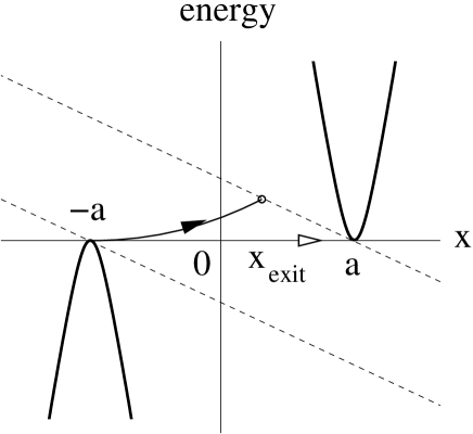
FIG. 4.: An inter-band tunneling (Zener breakdown) in a semiconductor with the energy gap $\varepsilon_{g}$ in a static electric field ${\cal E}_{0}$, shown by the open arrow. The tunneling length is $2a=\varepsilon_{g}/{\cal E}_{0}$. With a nonstationary field the path inside the forbidden region is shown by the full arrow.

FIG. 5.: (a) The cuts are shown by solid lines; (b) the contour $C_{q}$ terminates at the point $q$.

FIG. 6.: (a) At $x<-a$ two saddle point are involved which correspond to the incident and the reflected de Broglie waves; (b) for positive $x$ the saddle point relates to a particle after tunneling.

FIG. 7.: Thick curves relate to the condition $V(x,y)=E_{0}$. Normal tunneling between two classically allowed region $A$ and $B$, where $V(x,y)<E_{0}$, is described by the classical trajectory in imaginary time (thin curve) which meets the borders of $A$ and $B$ normally.

FIG. 8.: The potential energy of a particle in a quantum wire $V_{x}(x)+V_{y}(y)$ corresponds to the quantized motion in the radial $x$-direction (a) and an almost classical motion in the axis $y$-direction (b).

FIG. 9.: The potential energy $V(x,y)$ of a particle in the quantum wire in two dimensions.

FIG. 10.: Thick curves are determined by the condition $V(x,y)=E_{0}$. Normal tunneling “0” simply relates to the classical trajectory denoted by the dashed curve. Enhanced tunneling “1” is more complicated and consists of two steps: $A\rightarrow f$ and the classical trajectory $f\rightarrow B$. The vertical line goes from $y=y_{1}$ down to $y=y_{0}$.