Autler-Townes spectroscopy of the $5S_{1/2}-5P_{3/2}-44D$ cascade of cold ⁸⁵Rb atoms

Abstract

We study nonlinear optical effects in the laser excitation of Rydberg states. $5S_{1/2}$ and $5P_{3/2}$ levels of ⁸⁵Rb are coupled by a strong laser field and probed by a weak laser tuned to the $5P_{3/2}-44D$ Rydberg resonance. We observe high contrast Autler-Townes spectra which are dependent on the pump polarization, intensity and detuning. The observed behavior agrees with calculations, which include the effect of optical pumping.

With the birth of laser spectroscopy in the late 60s, new classes of nonlinear optical phenomena could be explored. One such measurement is the optical analogue of the Autler-Townes splitting autler , observed originally in the microwave domain. Following the work of Toschek and coworkers toschek69 ; toschek75a ; toschek75b there have been a number of studies of the Autler-Townes splitting in probe absorption, when a strong laser pump field drives a coupled transition in vapor cells or atomic beams picque ; vetter ; liao ; gray ; delsart ; sandeman . The introduction of laser cooling techniques such as the Magneto-Optical Trap (MOT) for neutral atoms has afforded precision measurements and optical spectroscopy not limited by Doppler effects or transit time broadening. Using frequency stabilized diode lasers, we extend previous Autler-Townes spectroscopy in MOTs atMOT1 ; atMOT2 ; atMOT3 to a new domain by using a high-lying Rydberg state with the excitation scheme shown in Fig. 1. As a consequence, the decay rate associated with the final level is all but eliminated. This work represents a step towards driving ground state-Rydberg transitions, which has been proposed as the working element in quantum information storage schemes dipblock1 ; dipblock2 .

The measurement is performed at 60 Hz inside a vapor cell MOT with a background pressure of $10^{-10}$ Torr. In each experimental cycle, the MOT lasers are turned off for 150 $\mu$s and the pump and probe fields of duration 10 $\mu$s are switched on simultaneously. The pump couples the 5$S_{1/2}F=3$ ground state and the 5$P_{3/2}F^{\prime}=4$ intermediate state ($\lambda\approx 780$ nm, saturation intensity $I_{\rm{sat}}$=1.64 mW/cm² and decay rate $\gamma_{2}/2\pi$=5.98 MHz,), while a linearly polarized probe field ($\lambda\approx 480$ nm) weakly couples the intermediate state to the 44$D$ Rydberg states. The pump beam is collimated to a FWHM of 2.2 mm after spatial filtering through a single mode optical fiber. The probe beam is focused to a size of 30 $\mu$m and aligned anti-parallel to the center of the pump beam. In this arrangement, the pump field intensity is approximately constant throughout the probe volume, and field inhomogeneity effects are minimized. The Zeeman shifts arising from the MOT magnetic field (gradient of 10 G/cm) are less than 2 MHz in the excitation volume, which is below the spectroscopic resolution. The probe laser is a frequency doubled external cavity diode laser locked to a temperature regulated and pressure tunable Fabry-Perot cavity. The Rydberg population (lifetime $\approx 60\mu$s) is monitored by counting electrons (gate = 100 $\mu$s) which originate from thermal ionization of Rydberg states with a Multi-Channel Plate (MCP) detector. The detection efficiency is estimated to be around 1.5 %.

Figure 1: Excitation scheme of ⁸⁵Rb from the 5$S_{1/2}$ ground state to the 44$D$ Rydberg states using linear and $\sigma^{+}$ pump fields. The squares of the Clebsch-Gordon coefficients associated with the transitions are indicated next to the lower arrows. The probe field is linearly polarized in direction parallel to the linear pump field.

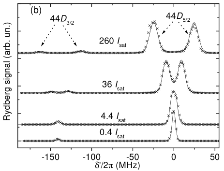
Figure 2: Measured Autler-Townes spectra ($\times$) for zero pump detuning. The 44$D_{3/2}$ and the 44$D_{5/2}$ lines are shown for pump intensities of 260$I_{\rm{sat}}$, 36$I_{\rm{sat}}$, 4.4$I_{\rm{sat}}$ and 0.4$I_{\rm{sat}}$ for $\sigma^{+}$ (a) and linear (b) pump polarizations. Solid lines are calculated lineshapes for intensities that have been adjusted by less than 10% from the measured intensities.

First, we consider the case of a resonant pump field (detuning, $\delta=\omega_{\rm{pump}}-\omega_{\rm{21}}=0$ where $\omega_{\rm{pump}}$ is the pump frequency and $\omega_{\rm{21}}$ is the transition frequency from $|1\rangle\rightarrow|2\rangle$). For a circularly polarized pump beam, the atoms are optically pumped into the $m_{F}=3$ ground state sublevel. Therefore, in steady state, the pump field drives only a single transition ($F=3,m_{F}=3\rightarrow F^{\prime}=4,m_{F^{\prime}}=4)$ having a Rabi frequency $\Omega_{c}=\Omega_{0}=\gamma_{2}\sqrt{\frac{s}{2}},$ where $s=I/I_{\rm{sat}}\$is the ratio of the pump intensity to the saturation intensity. For a pump field polarized linearly and parallel to the probe field’s polarization, there are four contributions to the spectra originating from states differing in their values of $\left|m_{F}\right|$ (see below). However, the dominant contribution to the lineshapes comes from states having $m_{F}=0,\pm 1$. Since the Rabi frequencies for these states, defined by

$$\Omega_{\ell}(m_{F})=\langle F=3,m_{F};1,0|F^{\prime}=4,m_{F^{\prime}}\rangle\Omega_{0},$$ (1)

are approximately equal, the Rabi splitting of the different components is not resolved and the average Rabi splitting is $\Omega_{\ell}\approx 0.74\Omega_{0}$. In Fig. 2, the spectra as a function of probe detuning $\delta^{\prime}=\omega_{\rm{probe}}-\omega_{32}$ are shown, where $\omega_{\rm{probe}}$ is the probe frequency and $\omega_{32}$ is the transition frequency from $|2\rangle\rightarrow|3\rangle$. At low pump intensities, we see two resonances corresponding to the 44$D_{3/2}$ and 44$D_{5/2}$ lines which are separated by 140 MHz calibration . The FWHM of these spectra lines are $\approx$ 4.5 MHz and can be attributed to the laser line width. As the pump intensity increases, the spectral lines broaden and the Autler-Townes components eventually separate. As shown in Fig. 3, the measured splittings are in excellent agreement with the Rabi frequencies ($\Omega_{c}=\Omega_{0}$ and $\Omega_{\ell}=0.74\Omega_{0}$), with $\Omega_{0}$ calculated using the measured pump beam intensities.

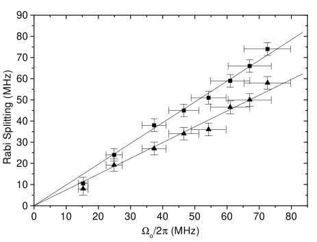
Figure 3: Measured Rabi splitting at zero pump detuning for the 44$D_{5/2}$ peaks for $\sigma^{+}$ ($\blacksquare$) and linear ($\blacktriangle$) pump light. Solid lines-theory.

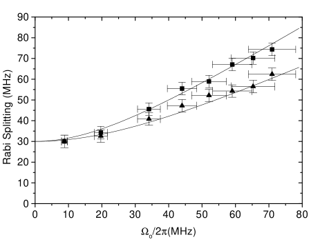
Figure 5: Measured Rabi splittings at 30 MHz (blue) pump detuning for the 44$D_{5/2}$ peaks for $\sigma^{+}$ ($\blacksquare$) and linear ($\blacktriangle$) pump light. Solid lines-theory.

With the pump beam detuned to the blue by $\delta/2\pi=30$ MHz, the two Autler-Townes components now have different amplitudes as shown in Fig. 4. The stronger component is red-detuned with respect to $\omega_{32}$ and corresponds to a two photon excitation process, while the weaker component corresponds to an off-resonant stepwise excitation. The splitting of the Autler-Townes peaks is given by the generalized Rabi frequency, $\sqrt{\Omega_{c}^{2}+\delta^{2}}$ and $\sqrt{\Omega_{l}^{2}+\delta^{2}}$ for $\sigma^{+}$ and linear pump polarizations, respectively. The measured Rabi splittings are in excellent agreement with the theoretical curves for both types of pump polarization, as shown in Fig. 5. The splittings for the $\sigma^{+}$ case are larger than those observed in the linear case owing to the larger Clebsch-Gordon coefficient.

Theoretical expressions for the Autler-Townes spectra are derived by solving the full set of density matrix equations to lowest order in the probe field, but to all orders of the pump field. It is assumed that the atom-field interaction time is sufficiently long for optical pumping to establish a steady-state distribution. In the case of circularly polarized pump field radiation, this implies that the pump field acts only between the $F=3,m_{F}=3$ and $F^{\prime}=4,m_{F^{\prime}}=4$ levels. The Autler-Townes signal is proportional to the total population in the 44$D$ manifold. Arbitrarily normalizing the signal to the $\sigma^{+}$ pump $D_{5/2}$ component (that is the integral over $\delta^{\prime}$ of this component is set equal to unity), we take as our signal

$$S_{c}=\frac{1}{\pi}\sum\limits_{J=3/2,5/2}\frac{w_{c}(J)}{w_{c}(5/2)}Re\left[\frac{\mu_{23}(J)}{\mu_{23}(J)\mu_{13}(J)+\left(\Omega_{0}^{2}/4\right)}\right],$$ (2)

where $\mu_{23}=(\gamma_{2}+\gamma_{3})/2+i\delta^{\prime}(J)$, $\mu_{13}=\gamma_{3}/2+i[\delta+\delta^{\prime}(J)]$, $\gamma_{3}\approx 16\times 10^{3}$s^-1 is the decay rate of the 44$D$ levels gamma3 , $\gamma=\gamma_{2}/2$ and $w_{c}(J)$ is a weighting function equal to

$$w_{c}(J)=18\left\{\begin{array}[]{ccc}2&1&1\\ 3/2&1/2&J\end{array}\right\}^{2}(2J+1)\sum_{F}\left(\left\langle 4,4;1,-1|F,3\right\rangle^{2}+\left\langle 4,4;1,1|F,5\right\rangle^{2}\right)\left\{\begin{array}[]{ccc}J&1&3/2\\ 4&5/2&F\end{array}\right\}^{2},$$ (7)

where $\left\{\ldots\right\}$ is a 6-J symbol. From this expression it follows that the ratio of the $J=$5/2 to 3/2 signal is 16.5. In the limit that the generalized Rabi frequency $\Omega=\sqrt{\Omega_{0}^{2}+\delta^{2}}\gg\gamma$, it is possible to reexpress the lineshape using a dressed atom approach salomaa as

$$S_{c}=\frac{1}{\pi}\sum\limits_{J=3/2,5/2}\frac{w_{c}(J)}{w_{c}(5/2)}\left[\frac{\Gamma_{1}\cos^{2}\theta}{\Gamma_{1}^{2}+\left(\delta^{\prime}(J)+\frac{\delta+\Omega}{2}\right)^{2}}+\frac{\Gamma_{2}\sin^{2}\theta}{\Gamma_{2}^{2}+\left(\delta^{\prime}(J)+\frac{\delta-\Omega}{2}\right)^{2}}\right],$$ (8)

where $\Gamma_{1}=\frac{\gamma_{3}}{2}\cos^{2}\theta+\frac{(\gamma_{2}+\gamma_{3})}{2}\sin^{2}\theta;\text{ \ }\Gamma_{2}=\frac{\gamma_{3}}{2}\sin^{2}\theta+\frac{(\gamma_{2}+\gamma_{3})}{2}\cos^{2}\theta$ and $\cos^{2}\theta=\frac{1}{2}\left(1+\frac{\delta}{\Omega}\right).$ In this form, it is clear that the ratio of the amplitude of the components of the Autler-Townes doublet for a given $J$ is equal to $\tan^{4}\theta$ and the ratio of the areas is equal to $\tan^{2}\theta$. The ratio of the areas is independent of laser line width. In Fig. 6 we plot the ratio of the areas versus tan${}^{2}\theta$ and see that experiment is in excellent agreement with theory.

For the case of a linearly polarized pump field, there are four contributions to each lineshape component from states differing in $\left|m_{F}\right|$. Using the normalization specified above, one finds the lineshape to be given by

$$S_{\ell}=\frac{1}{\pi}\frac{\gamma^{2}(1+s)+\delta^{2}}{\Omega_{0}^{2}/4}\sum\limits_{J=3/2,5/2}\sum\limits_{m}\frac{w_{\ell}(J,m)}{w_{c}(5/2)}\frac{\Omega_{\ell}(m)^{2}}{\gamma^{2}(1+\frac{s}{2})+\delta^{2}}Re\left[\frac{\mu_{23}(J)}{\mu_{23}(J)\mu_{13}(J)+\left[\Omega_{\ell}(m)^{2}/4\right]}\right]\rho_{1m,1m}^{(0)}$$ (9)

where

$$w_{\ell}(J,m) = 18\left\{\begin{array}[]{ccc}2&1&1\\ 3/2&1/2&J\end{array}\right\}^{2}(2J+1)\sum_{F}\left\langle 4,m;1,0|F,m\right\rangle^{2}\left\{\begin{array}[]{ccc}J&1&3/2\\ 4&5/2&F\end{array}\right\}^{2}$$ (14)

and $\rho_{1m,1m}^{(0)}$ is the steady state ground state population of sublevel $m$. Note that, in strong fields $\sum_{m}\rho_{1m,1m}^{(0)}\neq 1$, since there is non-negligible population in the $5P_{3/2}(F=4)$ level. It is also possible to write an expression analogous to Eq. (8) in a dressed basis by replacing $\left[\frac{\mu_{23}(J)}{\mu_{23}(J)\mu_{13}(J)+\left[\Omega_{\ell}(m)^{2}/4\right]}\right]$ in Eq. (9) with $\left[\frac{\Gamma_{1}(m)\cos^{2}\theta(m)}{\Gamma_{1}^{2}(m)+\left(\delta^{\prime}(J)+\frac{\delta+\Omega(m)}{2}\right)^{2}}+\frac{\Gamma_{2}(m)\sin^{2}\theta(m)}{\Gamma_{2}^{2}(m)+\left(\delta^{\prime}(J)+\frac{\delta-\Omega(m)}{2}\right)^{2}}\right]$, where the dressed state angle $\theta(m)$, the dressed state decay rates $\Gamma_{j}(m)$, and the generalized Rabi frequency $\Omega(m)$ are calculated using $\Omega_{\ell}(m)$ rather than $\Omega_{0}$.

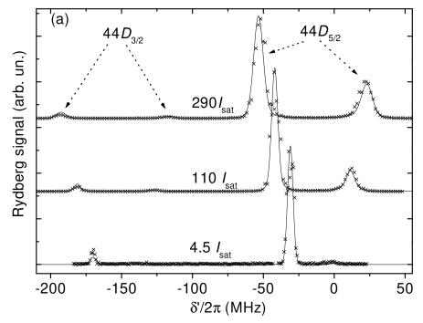
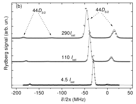
Figure 4: Measured Autler-Townes spectra ($\times$) at 30 MHz (blue) pump detuning. The 44$D_{3/2}$ and the 44$D_{5/2}$ lines are shown for pump intensities of 290$I_{\rm{sat}}$, 110$I_{\rm{sat}}$, and 4.5$I_{\rm{sat}}$ for $\sigma^{+}$ (a) and linear (b) pump polarizations. Solid lines are calculated lineshapes.

From the numerical solutions, we find that, for the range of parameters in our experiments, $\rho_{10,10}^{(0)}$ varies between 0.2 and 0.38, $\rho_{11,11}^{(0)}$ between 0.12 and 0.24, $\rho_{12,12}^{(0)}$ between 0.036 and 0.06, and $\rho_{13,13}^{(0)}$ between 0.0012 and 0.0044. Thus, the $m_{F}=0,\pm 1$ states give the dominant contributions. The ratio of the $D_{5/2}$ to $D_{3/2}$ component is found to be equal to 21 to within a few percent (it varies slightly with field intensity and detuning). The Rabi frequencies are equal to [$\Omega_{\ell}(0)=\sqrt{\frac{16}{28}}\Omega_{0},$ $\Omega_{\ell}(1)=\sqrt{\frac{15}{28}}\Omega_{0}$, $\Omega_{\ell}(2)=\sqrt{\frac{12}{28}}\Omega_{0},$ $\Omega_{\ell}(3)=\sqrt{\frac{7}{28}}\Omega_{0}$]; however since the $m=0,\pm 1$ substates dominate, the Rabi spitting is approximately equal to $\Omega_{e}=\frac{1}{2}[\Omega_{l}(0)+\Omega_{l}(1)]\approx 0.74\Omega_{0}$, and the ratio of the amplitude of the components of the Autler-Townes doublet for a given $J$ is equal roughly to $\tan^{4}\theta_{e}$, where $\theta_{e}$ is calculated using the effective Rabi frequency $\Omega_{e}$.

Since the laser line width is comparable with or larger than the level line widths, it is necessary to convolute the lineshapes with the spectral profile of the laser. Assuming that the width of the lines observed at the lowest intensities in Fig. 2 and Fig. 4 is attributable solely to laser line width, we find that the laser profile is described well by a Gaussian with FWHM of 4.5 MHz. This leads to excellent agreement between the experimental and theoretical curves at low pump intensities. However, to fit some of the curves in Fig. 2 and Fig. 4, it was necessary to increase the convolution width up to 10 MHz with increasing pump field intensity. We attribute this to the fact that the pump and probe beams were not perfectly aligned; inhomogeneities in the pump laser field then result in a distribution of Rabi frequencies, broadening the lines. The deviation of the data from the fits in Fig. 4 at low pump intensities can be attributed to incomplete optical pumping.

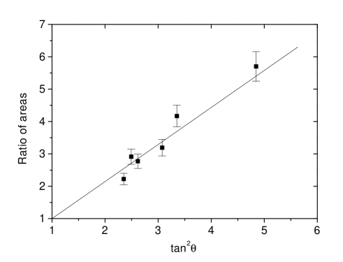
Figure 6: Ratio of areas of the two 44$D_{5/2}$ Autler-Townes components for $\sigma^{+}$ pump light. Solid line-theory.

In summary, we have observed high-resolution Autler-Townes Rydberg spectra of ⁸⁵Rb. The measured dependence of the Rabi splittings and line strengths on the pump field intensity, polarization and detuning are in excellent agreement with theory. In the near future, we plan to extend the off-resonant Autler-Townes measurements examined in this paper towards a pulsed, coherent two-photon excitation from the ground state into well defined Rydberg states. It should be possible to achieve two-photon Rabi oscillations between ground- and Rydberg states by starting with the detuned low-intensity regime of Fig. 4. The Rabi frequency of the upper $5P_{3/2}$ $\rightarrow$ $nD$ transition will have to be increased and the Rabi frequency of the lower transition $5S_{1/2}$ $\rightarrow$ $5P_{3/2}$ reduced, such that the population in the intermediate $5P$ state is minimized while a large two-photon Rabi frequency is maintained. The realization of Rabi oscillations or, equivalently, $\pi$- and $2\pi$-pulses pipulse to coherently transfer atoms into and out of individual Rydberg levels is of particular interest, because such operations are an important element in fast quantum gates that have been proposed in context with neutral-atom quantum computing dipblock1 ; dipblock2 .

This work was supported in part by NSF Grant Nos. PHY-0114336, PHY-0098016, PHY-9875553 and the U.S. Army Research Office Grant No. DAAD19-00-1-0412. J. R. G. acknowledges support from the Chemical Sciences, Geosciences and Biosciences Division of the Office of Basic Energy Sciences, Office of Science, U.S. Department of Energy.

References

- (1) S. H. Autler and C. H. Townes, Phys. Rev. 100, 703 (1955).
- (2) T. Hänsch et al, Z. Physik 226, 293 (1969).
- (3) A. Schabert, R. Keil and P. E. Toschek, Opt. Commun. 13, 265 (1975).
- (4) A. Schabert, R. Keil and P. E. Toschek, Appl. Phys. 6, 181 (1975).
- (5) J. L. Picque and J. Pinard, J. Phys. B 9, L77 (1976).
- (6) Ph. Cahuzac and R. Vetter, Phys. Rev. A 14, 270 (1976).
- (7) J. E. Bjorkholm and P. F. Liao, Opt. Commun. 21, 132 (1977).
- (8) H. R. Gray and C. R. Stroud, Opt. Commun. 25, 359 (1978).
- (9) C. Delsart, J. C. Keller and V. P. Kaftandjian, J. Phys. (Paris) 42, 529 (1981).
- (10) P. T. H. Fisk, H.-A. Bachor and R. J. Sandeman, Phys. Rev. A 33, 2418 (1986).
- (11) R. W. Fox et al, Opt. Lett. 18, 1456 (1993).
- (12) A. G. Sinclair, B. D. McDonald, E. Riis and G. Duxbury, Opt. Commun. 106, 207 (1994).
- (13) J. H. Marquardt, H. G. Robinson and L. Hollberg, J. Opt. Soc. Am. B 13, 1384 (1996).
- (14) D. Jaksch et al, Phys. Rev. Lett. 85, 2208 (2000).
- (15) M. D. Lukin et al, Phys. Rev. Lett. 87, 037901 (2001).
- (16) K. C. Harvey and B. P. Stoicheff, Phys. Rev. Lett. 38, 537 (1977)
- (17) In our 300K radiation field, the width of the final level is estimated to be s-1, i.e. slightly larger than the natural line width of 10.9s-1, but still much less than all other relevant widths.
- (18) P. R. Berman and R. Salomaa, Phys. Rev. A 25, 2667 (1982).
- (19) These s pulses are much longer than the ns pulses typically used in photon echo experiments. See, for example, A. Flusberg, R. Kachru, T. Mossberg and S. R. Hartmann, Phys. Rev. A 19, 1607 (1979).