An experimental observation of geometric phases for mixed states using NMR interferometry

Abstract

Examples of geometric phases abound in many areas of physics. They offer both fundamental insights into many physical phenomena and lead to interesting practical implementations. One of them, as indicated recently, might be an inherently fault-tolerant quantum computation. This, however, requires to deal with geometric phases in the presence of noise and interactions between different physical subsystems. Despite the wealth of literature on the subject of geometric phases very little is known about this very important case. Here we report the first experimental study of geometric phases for mixed quantum states. We show how different they are from the well understood, noiseless, pure-state case.

A quantum system can retain a memory of its motion when it undergoes a cyclic evolution, e.g its quantum state may acquire a geometric phase factor in addition to the dynamical one Panchar56 ; Ber84 . For pure quantum states this effect is well understood and it has been demonstrated in a wide variety of physical systems GPP89 . Its potential application to perform the fault-tolerant quantum computation has been the subject of more recent investigations JVEC00 ; Zan99 ; DCZ01 . In contrast, relatively little is known about geometric phases, and more generally, about quantum holonomies of mixed or entangled quantum states. Here we report an NMR experiment which constitutes the first experimental study of quantum holonomies for mixed quantum states. We observed and measured the geometric phase of a mixed state of a spin half nuclei. Our experimental data are in a good agreement with the recent theoretical predictions by Sjöqvist et al sjoqvist .

The geometric phase of pure states is an intriguing property of quantum systems undergoing parallel cyclic evolutions. The parallel transport of a particular vector $|\Psi\rangle$ implies no change in phase when $|\Psi(t)\rangle$ evolves into $|\Psi(t+dt)\rangle$, for some infinitesimal change of the parameter $t$. Although locally there is no phase change, the system may acquire a non-trivial phase after completing a closed loop parameterized by $t$. The origin of this phase can be traced to an underlying curvature of the parameter space, depending only on the geometry of the path and is resilient to certain dynamical perturbations of the evolution, e.g. it is independent of the speed of the evolution. Therefore, it is a potential method for performing intrinsically fault-tolerant quantum logic gates, a very desirable feature for practical implementations of quantum computation. However, quantum systems that interact with other systems, be it components in a quantum computer or otherwise, become entangled and cannot be described by a state vector $|\Psi\rangle$. In this context the notion of parallel transport and geometric phases must be extended to mixed quantum states.

Mathematically, Uhlmann was the first to address the issue of a mixed state holonomy  uhlmann . In his approach a system in a mixed state is embedded, as a subsystem, in a larger system that is in a pure state. Given a mixed state of the subsystem there are infinitely many corresponding pure states, known as purifications, of the larger system. Thus a cyclic evolution of the density operator pertaining to the subsystem induces infinitely many possible evolutions of the larger, purified system. Uhlmann singles out the evolution in which the purified state is transported in a maximally parallel manner. In order to satisfy this condition, one has to induce a suitable evolution on all auxiliary subsystems with which the original subsystem is entangled.

More recently Sjöqvist et al sjoqvist took a different approach in which there is no need for a direct reference to auxiliary subsystems EPSBO2002 . In their case each eigenvector of the initial density matrix is parallel transported independently and may acquire a geometric phase factor $\gamma_{n}$. The mixed state phase factor is then obtained as an average of the individual phase factors, weighted by their eigenvalues $p_{n}$,

$$ve^{i\gamma}=\sum_{n}p_{n}e^{i\gamma_{n}}.$$ (1)

This geometric phase factor can also be understood using purifications sjoqvist , though operations on auxiliary subsystems are unconstrained and as such they include Uhlmann’s approach as a special case.

Definitions, by definition, are never wrong or right, just more or less useful, thus we are not in a position to refute either of the two approaches. Here we investigate the holonomies of mixed quantum states and show that experimental data are consistent with the approach by Sjöqvist et al sjoqvist .

In our NMR experiment we focused on a mixed state of a spin half nuclei. Its density operator can be written in terms of the Bloch vector $\vec{r}$ and the Pauli matrices $\vec{\sigma}=\{\sigma_{x},\sigma_{y},\sigma_{z}\}$, as $\rho=\mbox{$\textstyle\frac{1}{2}$}(\leavevmode\hbox{\small 1\kern-3.8pt\normalsize 1}+\vec{r}\cdot\vec{\sigma})$. It represents a mixture of its two eigenvectors with eigenvalues $\mbox{$\textstyle\frac{1}{2}$}(1\pm r)$. The length of the Bloch vector $r$ gives the measure of the purity of the state – from maximally mixed $r=0$ to pure $r=1$. We use the gradient pulses to produce mixed states of different purities $r$. We then evolve the Bloch vector $\vec{r}$ so that it traces out a curve $C$ that subtends the solid angle $\Omega$. For spin half particles, Eq. (1) gives

$$ve^{i\gamma}=\cos\Omega/2+ir\sin\Omega/2.$$ (2)

This phase factor can be estimated from the visibility in an interference experiment sjoqvist . In our experiment we measure the geometric phase

$$\gamma=-\arctan\left(r\tan\frac{\Omega}{2}\right)$$ (3)

using an auxiliary spin half particle for the phase reference. A succinct description of the experiment is given in Fig. (1). Adopting the nomenclature from quantum information science we will sometimes refer to spin half particles as qubits.

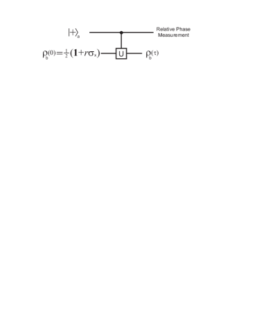
Figure 1: A quantum network describing the experiment. The top horizontal line represents an auxiliary spin half particle, or an auxiliary qubit, labelled as qubit “a”. The bottom line represents a qubit labelled as “b”, in state $\rho_{b}$ which undergoes a cyclic evolution induced by a unitary operation $U$. We choose our reference basis, for qubits“a” and “b”, to be states $|\uparrow\rangle$ and $|\downarrow\rangle$. They describe the spin state aligned with or against a static magnetic field $B_{0}$ applied in the $z$-direction. In this basis $|\pm\rangle=\frac{1}{\sqrt{2}}(|\uparrow\rangle\pm|\downarrow\rangle)$ thus the initial state of the auxiliary qubit is $|+\rangle_{a}$. Projectors $|\pm\rangle\langle\pm|$ can also be written as $\mbox{$\textstyle\frac{1}{2}$}(1\pm\sigma_{x})$.

The central element in Fig. (1) is the controlled-$U$ operation. In our case: the state $\rho_{b}$ traces out a closed path $C:t\in\left[0,\tau\right]\rightarrow\rho\left(t\right)=U\left(t\right)\rho\left(0\right)U^{{\dagger}}\left(t\right)$ on the Bloch sphere with a solid angle $\Omega$, but only when the auxiliary qubit is in state $|\uparrow\rangle_{a}$; when the auxiliary qubit is in state $|\downarrow\rangle_{a}$ the state $\rho_{b}$ is not affected. Such a controlled evolution can be realized in NMR with the scalar spin-spin coupling of the two spins. It effectively introduces a relative phase shift between the states $|\uparrow\rangle_{a}$ and $|\downarrow\rangle_{a}$ of the auxiliary qubit. In the experiment, the unitary operation which induces the cyclic motion completes the loop along the two geodesics, ABC and CDA, as illustrated in Fig.(2). It satisfies the parallel transport condition defined in sjoqvist and thus the dynamic phase vanishes.

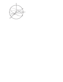
Figure 2: The cyclic path ABCDA subtends the solid angle $\Omega$ on the Bloch sphere. The solid angle can be changed by varying $\theta$ - the angle of inclination between the $x,y$-plane and the ABC plane (or the ADC plane). In the experiment the Bloch vectors of different lengths $r$ follow the path identical to the ABCDA but right below it, at the distance $r$ from the centre of the sphere. The two Bloch vectors corresponding to the two eigenvectors of the density operator are the unit vectors $\pm\vec{r}/r$. In the cyclic evolution one of them follows the path ABCDA and subtends the solid angle $\Omega$ and the other follows the path symmetrically on the opposite side of the sphere and subtends the solid angle $-\Omega$.

In our experiment the geometric phase for mixed states was observed using an NMR spectrometer. We used a 0.5 ml, 200 mmol sample of Carbon-13 labelled chloroform (Cambridge Isotopes) in d₆ acetone. The single ${}^{13}C$ nucleus was used as the auxiliary qubit while the ${}^{1}H$ nucleus was used as the qubit on which the cyclic evolution was executed. The reduced Hamiltonian for this two-spin system is, to an excellent approximation, given by

$$H=\omega_{a}I_{z}^{a}+\omega_{b}I_{z}^{b}+2\pi J\;I_{z}^{a}I_{z}^{b}.$$ (4)

The first two terms in the Hamiltonian describe the free precession of spin “a” (${}^{13}C$) and spin “b” (${}^{1}H$) around the magnetic field $B_{0}$ with frequencies $\omega_{a}/2\pi\approx 100$MHz and $\omega_{b}/2\pi\approx 400$MHz. The $I_{z}^{a}$ and $I_{z}^{b}$ are the $z$-components of the angular momentum operator for “a” and “b” respectively ($I_{z}\equiv\mbox{$\textstyle\frac{1}{2}$}\sigma_{z}$). The third term of the Hamiltonian describes a scalar spin-spin coupling of the two spins with $J=214.5$Hz. In our experiment, we varied the solid angle $\Omega$, and for each $\Omega$ we measured the geometric phase $\gamma$ for twelve values of $r=\cos\frac{n\pi}{12},\;n=0,1,\ldots,11$.

Let us now describe step by step different stages of the experiment in more detail.

(E1) Preparation of the initial state: Initially the two qubits are in thermal equilibrium with the environment and their state is described by the density operator $\rho_{th}\propto\sigma_{z}^{a}+4\sigma_{z}^{b}$. We use the spatial averaging technique cory to create the effective pure state $|\uparrow\rangle_{a}\otimes|\uparrow\rangle_{b}$ or, in the density operator form, $\mbox{$\textstyle\frac{1}{2}$}(1+\sigma_{z}^{a})\otimes\mbox{$\textstyle\frac{1}{2}$}(1+\sigma_{z}^{b})$. The sequence of operations leading to this state, reading from the left to the right, is as follows,

$$R_{x}^{b}\left(\pi/3\right)-G_{z}-R_{x}^{b}\left(\pi/4\right)-\frac{1}{2J}-R_{-y}^{b}\left(\pi/4\right)-G_{z},$$ (5)

where $R_{x}^{b}(\alpha)=e^{-i\alpha\sigma_{x}/2}$ denotes a selective pulse that rotates the spin $b$ around the $x$-axis by angle $\alpha$ (and $R_{-x}^{b}(\alpha)\equiv R_{x}^{b}(-\alpha)$), $G_{z}$ is the pulsed field gradient along the $z$-axis (it annihilates the transverse magnetizations), and $\frac{1}{2J}$ represents just a time interval of $1/\left(2J\right)$. Note that the above pulse sequence is different from the one described in cory because we used a heteronuclei rather than a homonuclei sample. The subsequent pulse sequence

$$R_{x}^{b}\left(n\pi/12\right)-G_{z}-R_{-y}^{a}\left(\pi/2\right)-R_{-y}^{b}\left(\pi/2\right)$$ (6)

generates the desired initial state

$$\rho_{ab}\left(0\right)\equiv\rho_{a}\left(0\right)\otimes\rho_{b}\left(0\right)=\mbox{$\textstyle\frac{1}{2}$}(\leavevmode\hbox{\small 1\kern-3.8pt\normalsize 1}+\sigma_{x}^{a})\otimes\mbox{$\textstyle\frac{1}{2}$}(\leavevmode\hbox{\small 1\kern-3.8pt\normalsize 1}+r\sigma_{x}^{b})$$ (7)

with purity $r=\cos(n\pi/12);\;n=0,1,\cdots,11$, which is set by the rotation angle $n\pi/12$ of the selective pulse $R_{x}^{b}(n\pi/12)$.

(E2) The controlled-$U$ operation: This operation is implemented setting the oscillation frequency $\omega_{b}^{\prime}=\omega_{b}-\pi J$, so that the Hamiltonian of qubit $b$ in the rotating frame with angular frequency $\omega_{b}^{\prime}$ can be written as $H_{b}(0)=(\omega_{b}-\omega_{b}^{\prime}\pm\pi J)\;I_{z}^{b}$. The $\pm$ sign is determined by the state of qubit $a$. If qubit $a$ is in state $|\uparrow\rangle_{a}$ then $H_{b}(0)=0$; if qubit $a$ is in state $|\downarrow\rangle_{a}$ then $H_{b}(0)=2\pi J\;I_{z}^{b}$. Subsequently we use the following pulse sequence to implement the cyclic evolution,

$$R_{-x}^{b}\left(\theta\right)-\frac{1}{2J}-R_{-x}^{b}\left(\pi-2\theta\right)-\frac{1}{2J},$$ (8)

where $\theta=\Omega/4$ is the inclination angle (see Fig.(2)). The effect of this evolution is illustrated in Fig.(2). The two eigenstates of $\rho_{b}(0)$, namely $|\pm\rangle_{b}$, trace out a path which encompasses the solid angle $\Omega$ and acquire geometric phases $|\pm\rangle_{b}\mapsto e^{\mp i\frac{\Omega}{2}}|\pm\rangle_{b}$. Since the path follows geodesics, the dynamical phase disappears. Thus the auxiliary qubit acquires the phase factor $e^{\mp i\frac{\Omega}{2}}$, i.e. $\frac{1}{\sqrt{2}}(|\uparrow\rangle+|\downarrow\rangle)\mapsto\frac{1}{\sqrt{2}}(|\uparrow\rangle+e^{\mp i\frac{\Omega}{2}}|\downarrow\rangle)$, with the probability $\mbox{$\textstyle\frac{1}{2}$}(1\pm r)$. Their averaging gives the phase factor as in Eq.(2).

(E3) Measurement: In the experiment we use a phase sensitive detector to measure the phase $\gamma$ relative to the reference phase of the initial state $|+\rangle_{a}$.

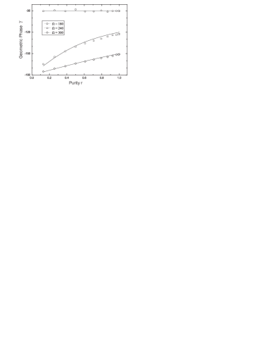
Figure 3: Summary of experimentally determined geometric phase $\gamma$ as a function of purity of the mixed state for three different solid angles $\Omega$. The solid lines correspond to the theoretical result: $\gamma=-\arctan\left(r\tan\frac{\Omega}{2}\right)$.

Fig. 3 shows a plot of $\gamma$ versus the purity of mixed state for the three different solid angles $\Omega$. The experimental data and the theoretical prediction are in a very good agreement. The small errors are due to inhomogeneity of magnetic field and imperfect pulses.

All experiments were conducted at room temperature and pressure on Bruker AV-400 spectrometer. In our experiment, all the pulses are square and are of several microseconds duration. The spin-spin relaxation times are $0.3$s for carbon and $0.4$s for proton, respectively. In each experiment, the time used for the cyclic parallel transport evolution is about $4.7$ms, which is well within the decoherence time.

To summarize, we have experimentally observed geometric phases for mixed states which are in accordance with the theoretical predictions. In the future, we should be able to extend the study of geometric phases to the non-unitary regime which is especially pertinent to their application to fault tolerant quantum computation ESBOP2002 .

- (1) S. Pancharatnam, Proc. Indian Acad. Sci. A 44, 247 (1956).
- (2) M. V. Berry, Proc. Roy. Soc. A 392, 45 (1984).
- (3) A. Shapere and F. Wilczek, Geometric phases in Physics, World Scientific, Singapore (1989).
- (4) J. A. Jones, V. Vedral, A. Ekert and G. Castagnoli, Nature 403, 869 (2000).
- (5) P. Zanardi, M. Rasetti, Phys. Lett. A 264, 94 (1999).
- (6) L. M. Duan, J. I. Cirac, P. Zoller, Science 292, 1695 (2001).
- (7) E. Sjöqvist, A.K. Pati, A. Ekert, J.S. Anandan, M. Ericsson, D.K.L. Oi and V. Vedral, Phys. Rev. Lett. 85, 2845 (2000).
- (8) A. Uhlmann, Rep. Math. Phys. 24, 229 (1986).
- (9) M. Ericsson, A. K. Pati, E. Sjöqvist, J. Brännlund and D. K. L. Oi, arXiv.org electronic pre-print quant-ph/0206063 (2002).
- (10) D. G. Cory, M. D. Price and T. F. Havel, Physica D 120, 82 (1998).
- (11) M. Ericsson, E. Sjöqvist, J. Brännlund, D. K. L. Oi and A. K. Pati, arXiv.org electronic pre-print quant-ph/0205160 (2002).