Abstract

Broadband implementations of time-optimal geodesic pulse elements are introduced for the efficient creation of effective trilinear coupling terms for spin systems consisting of three weakly coupled spins 1/2. Based on these pulse elements, the time-optimal implementation of indirect SWAP operations is demonstrated experimentally. The duration of indirect SWAP gates based on broadband geodesic sequence is reduced by 42.3% compared to conventional approaches.

1 Introduction

In the absence of relaxation, nuclear magnetic resonance (NMR) experiments consist of a sequence of unitary transformations of the density operator representing the spin system of interest [1]. An important goal of both theoretical and practical interest is the design of pulse sequences that can generate a desired unitary transformation as fast as possible, in order to reduce losses due to relaxation. This poses the problem of time-optimal control of quantum systems [2, 3, 4], which is of interest for coherent spectroscopy in general, as well as for quantum information processing [5].

Here, we focus on the realization of effective propagators that correspond to the action of an effective Hamiltonian with trilinear coupling terms which simulate a three-spin interaction in spin chains consisting of three weakly coupled spins 1/2 (Ising coupling). In the context of NMR polarization-transfer experiments, methods for creating such effective trilininear Hamiltonians have been developed and used for many years [6, 7]. One approach to create such effective Hamiltonians is based on the decoupling of certain interactions during the pulse sequence [3, 8, 9]. An earlier, more efficient approach does not rely on decoupling [6, 7]. Recently, further improved sequences [3] were derived which also avoid decoupling. Even larger time savings are possible by using geodesic pulse sequences [3] that can be shown to be time-optimal. However, so far the geodesic pulse sequences were based on weak rf pulses which severely limited the range of frequency offsets for which the experiment is functional. In order to pave the way for practical applications of these time-optimal pulse elements, we developed broadband versions of the time-optimal geodesic sequence. Time-optimal indirect SWAP operations [3] were realized experimentally in a three-spin system, demonstrating the superior performance of the new sequences.

2 Theory

We consider a chain of three heteronuclear spins with coupling constants $J_{12}=J_{23}=J$, $J_{13}=0$ and offsets $\nu_{1}$, $\nu_{2}$, and $\nu_{3}$. In a multiple-rotating frame [1], the corresponding free evolution Hamiltonian ${\cal H}_{0}$ is in general given by

$${\cal H}_{0}={\cal H}_{c}+{\cal H}_{\it off},$$ (1)

with the coupling term

$${\cal H}_{\rm c}=2\pi JI_{1z}I_{2z}+2\pi JI_{2z}I_{3z}$$ (2)

and the offset term

$${\cal H}_{\it off}=2\pi\nu_{1}I_{1z}+2\pi\nu_{2}I_{2z}+2\pi\nu_{3}I_{3z}.$$ (3)

The same Hamiltonian is valid if e.g. the first and third spins are homonuclear and the second spin is heteronuclear (vide infra).

Many applications in NMR spectroscopy [6, 7] and NMR quantum computing [10, 11, 12] require unitary transformations of the form

$${\cal U}_{\alpha\beta\gamma}(\kappa)=\exp\{-{\rm i}\ 2\pi\ \kappa\ I_{1\alpha}I_{2\beta}I_{3\gamma}\},$$ (4)

where $\alpha$, $\beta$, $\gamma$ can be $x$, $y$ or $z$. The time $\tau$ required to realize such a propagator depends on the pulse sequence and is a function of $\kappa$ (see Table 1). The propagator ${\cal U}_{\alpha\beta\gamma}(\kappa)$ can also be expressed as

$${\cal U}_{\alpha\beta\gamma}(\kappa)=\exp\{-{\rm i}\ \tau(\kappa)\ {\cal H}_{\alpha\beta\gamma}\},$$ (5)

where ${\cal H}_{\alpha\beta\gamma}$ corresponds to an effective trilinear coupling Hamiltonian of the form

$${\cal H}_{\alpha\beta\gamma}=2\pi J_{\it eff}(\kappa)\ I_{1\alpha}I_{2\beta}I_{3\gamma},$$ (6)

and the effective trilinear coupling constant $J_{\it eff}(\kappa)$ is defined by

$$J_{\it eff}(\kappa)={{\kappa}\over{\tau(\kappa)}}.$$ (7)

For practical applications, $\tau(\kappa)$ should be as short as possible and hence the effective coupling constant $J_{\it eff}(\kappa)$ and the scaling factor

$$s(\kappa)={{J_{\it eff}(\kappa)}\over{J}}={{\kappa}\over{J\ \tau(\kappa)}}$$ (8)

should be as large as possible. For $0\leq\kappa\leq 1$, the theoretical limit $\tau^{\ast}(\kappa)$ for the minimum time required to create a propagator ${\cal U}_{\alpha\beta\gamma}(\kappa)$ is given by [3]

$$\tau^{\ast}(\kappa)={\sqrt{\kappa(4-\kappa)}\over{2J}},$$ (9)

which corresponds to a maximum possible scaling factor

$$s^{\ast}(\kappa)={{2\kappa}\over{\sqrt{\kappa(4-\kappa)}}}.$$ (10)

It is sufficient to consider $\tau^{\ast}(\kappa)$ and $s^{\ast}(\kappa)$ only for $0\leq\kappa\leq 1$, because $\tau^{\ast}(2n\pm\kappa)=\tau^{\ast}(\kappa)$, where $n$ is an arbitrary integer [3].

Schematic pulse sequences corresponding to four different approaches for the creation of ${\cal U}_{zzz}(\kappa)$ are shown in Fig. 1. These sequences can be further streamlined by reducing the number of pulses using well known rules (vide infra).

Sequence A with duration

$$\tau_{A}(\kappa)={{2+\kappa}\over{2J}}$$ (11)

is based on the identity [3]

$${\cal U}_{zzz}(\kappa)={\rm exp}\{-{\rm i}\pi I_{1z}I_{2x}\}\ \exp\{-{\rm i}\pi\ \kappa\ I_{2y}I_{3z}\}\ {\rm exp}\{{\rm i}\pi I_{1z}I_{2x}\}.$$ (12)

Equivalent sequences [8] with the same duration $\tau_{A}(\kappa)$ but with less pulses can be constructed based on the identity

$${\cal U}_{zzz}(\kappa)=V_{A}\ \exp\{-{\rm i}\pi\ \kappa\ I_{2z}I_{3z}\}\ V_{A}^{-1}.$$ (13)

with

$$V_{A}={\rm exp}\{-{\rm i}{{\pi}\over{2}}I_{2x}\}\ {\rm exp}\{-{\rm i}\pi I_{1z}I_{2z}\}\ {\rm exp}\{-{\rm i}{{\pi}\over{2}}I_{2y}\}.$$ (14)

Equivalant sequence with the same duration $\tau_{A}(\kappa)$ can also be constructed using CNOT operations [9].

Sequence B with duration

$$\tau_{B}(\kappa)={{1}\over{J}}$$ (15)

is based on the identity [6, 7]

$${\cal U}_{zzz}(\kappa)=V_{B}\ \exp\{-{\rm i}\ {{\pi}\over{2}}\ \kappa\ I_{2x}\}\ V_{B}^{-1}.$$ (16)

with

$$V_{B}={\rm exp}\{-{\rm i}\ {{\pi}\over{2}}\ I_{2y}\}\ {\rm exp}\{-{\rm i}\ \pi\ (I_{1z}I_{2z}+I_{2z}I_{3z})\}.$$ (17)

Sequence C with duration

$$\tau_{C}(\kappa)={{1+\kappa}\over{2J}}$$ (18)

is based on the identity [3]

$${\cal U}_{zzz}(\kappa)=V_{C}\ \exp\{-{\rm i}\ \pi\ \kappa\ (I_{1z}I_{2y}+I_{2y}I_{3z})\}\ V_{C}^{-1}\ {\rm exp}\{{\rm i}\ {{\pi}\over{2}}\ \kappa\ I_{2z}\}.$$ (19)

with

$$V_{C}={\rm exp}\{-{\rm i}\ {{\pi}\over{2}}\ (I_{1z}I_{2x}+I_{2x}I_{3z})\}.$$ (20)

Finally, the time-optimal sequence D with duration

$$\tau_{D}(\kappa)=\tau^{\ast}(\kappa)={\sqrt{\kappa(4-\kappa)}\over{2J}}$$ (21)

is based on the identity [3]

$${\cal U}_{zzz}(\kappa)=V_{D}\ W\ \exp\{-{\rm i}\pi\sqrt{\kappa(4-\kappa)}(I_{1z}I_{2z}+I_{2z}I_{3z})+{\rm i}\pi(2-\kappa)I_{2x}\}\ V_{D}^{-1}$$ (22)

with

$$V_{D}={\rm exp}\{-{\rm i}\ {{\pi}\over{2}}\ I_{2y}\}$$ (23)

and

$$W={\rm exp}\{-{\rm i}\pi(2-{{\kappa}\over{2}})I_{2x}\}.$$ (24)

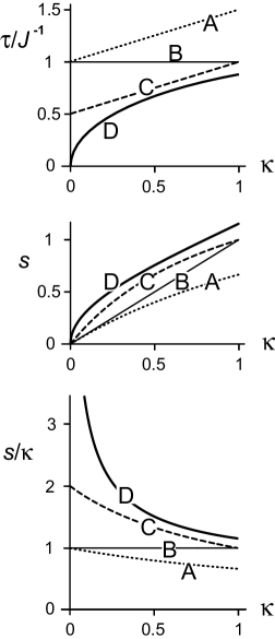
Figure 2: Durations $\tau(\kappa)$ (top panel), scaling factors $s=J_{\it eff}(\kappa)/J=\kappa/J\tau(\kappa)$ (middle panel), and relative scaling factors $s/s_{B}=s/\kappa$ (bottom panel) of the four basic pulse sequences A-D shown in Fig. 1.

The durations $\tau(\kappa)$ and scaling factors $s(\kappa)=J_{\it eff}(\kappa)/J$ of sequences A-D are shown in Fig. 2 and are summarized in Table 1. In all four sequences, $I_{2}$-selective pulses are required. In addition, $I_{1}$-selective and $I_{3}$-selective 180^∘ pulses are required in sequence A for selective decoupling of $J_{12}$ and $J_{23}$ during parts of the pulse sequence. In contrast, sequences B-D do not require such $I_{1}$-selective or $I_{3}$-selective pulses, which simplifies the experimental implementation of these pulse sequences if spins $I_{1}$ and $I_{3}$ are homonuclear. These sequences are also suitable for applications, where spins $I_{1}$ and $I_{3}$ are equivalent, as in I₂S spin systems [6, 7]. Furthermore, the fact that decoupling is avoided in sequences B-D makes these experiments considerably more efficient than sequence A (vide infra). Sequence B is a straight-forward generalization of a well-known pulse sequence developped initially [6, 7] for the special case of $\kappa=1$. Sequence C, which has been proposed recently [3], is more efficient than sequence B. The geodesic pulse sequence (sequence D) has the shortest possible duration for all values of $\kappa$ [3], see Fig. 2 A (top panel). For $\kappa\rightarrow 0$, the duration of the geodesic pulse sequence approaches 0, in contrast to sequences A-C. Fig. 2 (middle panel) shows the scaling factors $s(\kappa)$ and Fig. 2 (bottom panel) shows the relative scaling factors $s(\kappa)/\kappa$ compared to the scaling factor of sequence B ($s_{B}=\kappa$). For $\kappa=1$, the scaling factor $s$ of the geodesic sequence is 73.2% larger compared to sequence A and about 15.5% larger compared to sequences B and C. As $\kappa$ approaches 0, the scaling factor $s$ of the geodesic pulse sequence becomes infinitely larger than the scaling factors of sequences A-C. For example, for $\kappa=0.01$ the scaling factor $s$ of the geodesic sequence is already about a factor of 10 larger compared to sequences A and B and about a factor of 5 larger compared to sequence C.

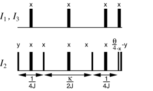
Figure 3: Broadband version of sequence C shown in Fig. 1.

The basic pulse sequences shown in Fig. 1 only create the desired unitary transformations ${\cal U}_{zzz}(\kappa)$ if all spins are on-resonance in a multiple-rotating frame, i.e. if ${\cal H}_{\it off}=0$ (c.f. Eq. 3). However, for most practical applications, a finite offset range must be covered by the pulse sequences. Broadband versions of sequence B can be found in the literature [6, 7]. Broadband versions of sequences A [8] and C can be created in a straight-forward way by inserting additional $\pi$ pulses in the existing delays to refocus chemical shift evolution. For example, a broadband version of sequence C is shown in Fig. 3. The robustness of the broadband sequence with respect to rf inhomogeneity and offsets can be further improved by using the $x$, $-x$, $-x$, $x$ cycle [14] for the phases of the four $\pi$ pulses which are applied to spins $I_{1}$ and $I_{3}$.

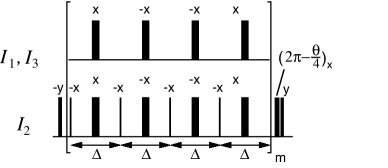
Figure 4: Broadband version of the geodesic sequence shown in Fig. 1D for the time-optimal implementation of ${\cal U}_{zzz}(\kappa)$. The pulse sequence element in brackets has a duration of 4$\Delta$ and is repeated $m$ times. The narrow vertical bars in the bracket correspond to hard pulses with flip angles $2\pi\nu_{w}\tau^{\ast}/n$ and $\Delta=\tau^{\ast}/n$ with $n=4m$.

Although no delays exist in the ideal geodesic pulse sequence shown in Fig. 1D, delays can be introduced by replacing the weak pulse with amplitude $\nu_{w}=(2-\kappa)J/\sqrt{\kappa(4-\kappa)}$, duration $\tau^{\ast}(\kappa)=\sqrt{\kappa(4-\kappa)}/(2J)$, and flip angle $\alpha_{w}=\nu_{w}t_{w}2\pi=(2-\kappa)\pi$ by $n$ hard pulses with flip angle $\alpha_{w}/n$ and $n$ delays of duration $\Delta=\tau^{\ast}(\kappa)/n$. In the limit of $n\rightarrow\infty$, this DANTE-type (Delays alternating with Nutations for Tailored Excitation) [13] pulse sequence creates the same effect as the weak pulse and with the same limited bandwidth. For the present application, the DANTE-type sequence approaches the ideal sequence if $\Delta\ll 1/J$. By inserting $\pi$ pulses in the delays of the DANTE sequence (c.f. Fig. 4), a broadband version of the geodesic pulse sequence can be created. As shown in Fig. 4, the robustness of the broadband geodesic sequence with respect to rf inhomogeneity and offset can be improved by using cycles or supercycles such as $x$, $-x$, $-x$, $x$ [14] for the phases of each set of four $180^{\circ}$ pulses.

In addition to applications in polarization transfer experiments [6, 7], propagators corresponding to trilinear effective coupling terms are useful in the field of quantum information processing. For example, so-called $\Lambda_{2}$ gates [15] can be implemented efficiently based on $U_{zzz}(\kappa)$ for $\kappa=1$. Here, we focus on the implementation of SWAP operations [16, 17, 18] that make it possible to exchange arbitrary spin states of two spins in a coupling network. For weakly coupled spins such as in the spin system defined in Eq. (2), a direct SWAP gate such as ${\it SWAP}(1,2)$ or ${\it SWAP}(2,3)$ between directly coupled spins $I_{1}$ and $I_{2}$, or between $I_{2}$ and $I_{3}$ has a minimum duration of [2]

$$\tau_{{\it SWAP}(1,2)}=\tau_{{\it SWAP}(2,3)}=3/(2J).$$ (25)

An indirect SWAP operation ${\it SWAP}(1,3)$ between spins $I_{1}$ and $I_{3}$, which are not directly coupled, can always be realized based on the following combination of the direct SWAP gates ${\it SWAP}(1,2)$ and ${\it SWAP}(2,3)$:

$${{\it SWAP}}(1,3)={{\it SWAP}}(1,2)\ {{\it SWAP}}(2,3)\ {{\it SWAP}}(1,2)$$ (26)

with an overall duration

$$\tau^{conv}_{{\it SWAP}(1,3)}=2\ \tau_{{\it SWAP}(1,2)}+\tau_{{\it SWAP}(2,3)}=9/(2J).$$ (27)

However, the time-optimal realization of the indirect SWAP operation ${\it SWAP}(1,3)$ has a duration of only [3]

$$\tau^{\ast}_{{\it SWAP}(1,3)}=3\ \tau^{\ast}(1)=3\sqrt{3}/(2J)$$ (28)

and hence requires only 57.7 $\%$ of the duration $\tau^{conv}_{{\it SWAP}(1,3)}$ of the conventional sequence (c.f. Eq. 27). This approach is based on the time-optimal realization of propagators ${\cal U}_{\alpha\beta\gamma}(\kappa)$ (c.f. Eq. 5), which create the desired indirect ${\it SWAP}(1,3)$ gate by the following sequence of operations [3]:

$${\cal U}_{{\it SWAP}(1,3)}={\cal U}_{zzz}(1)\ {\cal U}_{yzy}(1)\ {\cal U}_{xzx}(1)\ \exp({\rm i}\frac{\pi}{2}I_{2z}).$$ (29)

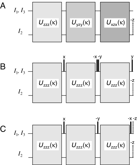
Figure 5: Pulse sequences implementing the indirect SWAP operation ${\cal U}_{{\it SWAP}(1,3)}$ for $\kappa=1$. (A) Schematic implementation according to Eq. 29, (B) equivalent implementation based on pulse sequence elements (c.f. Fig. 1) that create the propagator ${\cal U}_{zzz}(\kappa)$, (C) streamlined pulse sequence with a minimum number of $90^{\circ}$ pulses.

Note that all terms in Eq. 29 mutually commute and hence in experimental implementations the order of the corresponding pulse sequnce elements is arbitrary. Based on pulse sequence elements for the realization of ${\cal U}_{zzz}(\kappa)$, the sequence of propagators in Eq. (29) can be realized in a straight-forward way by the pulse sequence shown in Fig. 5 C. The final $90^{\circ}_{-z}$ rotations can either be implemented by a composite pulse such as $90^{\circ}_{x}\ 90^{\circ}_{y}\ 90^{\circ}_{-x}$or by adjusting the phases of all following pulses and of the receiver [19]. In general, $z$ rotations (by angle $\varphi$) can be implemented by an additional phase shift (by angle $-\varphi$) of all following r.f. pulses that are applied to this spin and of the receiver phase for this spin [19].

3 Experiments

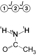
Figure 6: The model system (top) consisting of a chain of three coupled spins 1/2 with $J_{12}=J_{23}=J$ and $J_{13}=0$ is approximated by the spins of the amino moiety (printed in boldface) of [¹⁵N]-acetamide (bottom).

In order to test the performance of the new geodesic pulse sequences, we used the spin system of the amino moiety of [¹⁵N]-acetamide as a model system (see Fig. 6) that corresponds closely to the model Hamiltonian ${\cal H}_{0}={\cal H}_{c}+{\cal H}_{\it off}$ defined in Eqs. (1-3). [¹⁵N]-acetamide (Chemotrade GmbH) was dissolved in DMSO-d6 and all measurements were performed on a Bruker 600 MHz DMX spectrometer (Bruker Analytik GmbH) at a temperature of 298 K. Here, spins $I_{1}$ and $I_{3}$ correspond to the amino protons, whereas $I_{2}$ corresponds to the ¹⁵N spin with $J_{12}=$ 88.8 Hz $\approx J_{23}=$ 87.3 Hz $\gg J_{13}=2.9$ Hz. Additional ${}^{4}J(^{1}H,^{1}H)$ and ${}^{3}J(^{1}H,^{15}N)$couplings (0.7 Hz and 1.2 Hz) of $I_{1}$ and $I_{2}$ to the methyl protons of [¹⁵N]-acetamide are about two orders of magnitude smaller than the ${}^{1}J(^{1}H,^{15}N)$ couplings.

Compared to a fully heteronuclear spin system, the relatively small frequency difference $\Delta\nu_{13}=358$ Hz of the amino protons (spins $I_{1}$ and $I_{3}$) makes it difficult to apply short selective pulses to spin $I_{1}$ that do not affect spin $I_{3}$ (and vice versa) as required in sequence A (and also for its broadband implementation using additional refocussing pulses). In our experiments, we implemented spin-selective proton pulses by a combination of hard pulses and delays. For example, if spin $I_{1}$ is irradiated on resonance, a selective 180${}^{\circ}_{x}(I_{1})$ pulse can be implemented by the pulse sequence element

90${}^{\circ}_{x}(I_{1},I_{3})$   -  $\delta$  -   180${}^{\circ}_{x}(I_{2})$   -  $\delta$  -   180${}^{\circ}_{x}(I_{2})$ 90${}^{\circ}_{x}(I_{1},I_{3})$,

where $\delta=2/(4\Delta\nu_{13})=698$ $\mu$s. Similarly, a selective 180${}^{\circ}_{x}(I_{3})$ pulse can be implemented by the same pulse sequence element if the last 90${}^{\circ}_{x}(I_{1},I_{3})$ pulse is replaced by 90${}^{\circ}_{-x}(I_{1},I_{3})$.

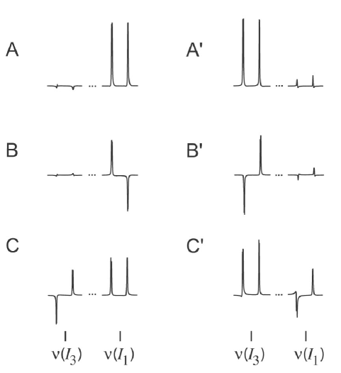
Figure 7: ¹H spectra of the amino protons (spins $I_{1}$ and $I_{3}$) of [¹⁵N]-acetamide before (A-C) and after (A^′-C^′) an indirect ${\it SWAP}(1,3)$ operation based on Fig. 5 C and the broadband sequence shown in Fig. 3 for the creation of ${\cal U}_{zzz}(\kappa)$ for $\kappa=1$. The initial spin states were prepared to be (A) $\rho(0)=I_{1x}$, (B) $\rho(0)=2I_{1x}I_{2z}$, and (C) $\rho(0)=I_{1x}+2I_{2z}I_{3x}$, respectively.

Based on broadband versions of sequences A, C, and D, we implemented the sequence shown in Fig. 5 C, which realizes a ${\it SWAP}(1,3)$ operation for $\kappa=1$. Note that the sequence of Fig. 5 C still allows for a variation of $\kappa$, which makes it possible to test the theoretically expected $\kappa$ dependence of the sequences (vide infra). For $\kappa=1$, the sequences for the ${\it SWAP}(1,3)$ gate were successfully tested for a large number of initial states of the spin system. Three illustrative examples are presented in Fig. 7, where ¹H spectra of the amino protons (spins $I_{1}$ and $I_{3}$) of [¹⁵N]-acetamide are shown. Left (A-C) and right (A^′-C^′) spectra reflect the states before and after an indirect ${\it SWAP}(1,3)$ operation, repectively. The initial spin states were prepared to be $\rho(0)=I_{1x}$ (c.f. Fig. 7A), (B) $\rho(0)=2I_{1x}I_{2z}$ (c.f. Fig. 7 B), and (C) $\rho(0)=I_{1x}+2I_{2z}I_{3x}$ (c.f. Fig. 7 C). As expected, the states of the two proton spins (spins $I_{1}$ and $I_{3}$) are swapped for arbitrary initial states.

In order to compare the durations and $\kappa$ dependence of the indirect ${\it SWAP}(1,3)$ sequences, we measured the efficiency of inphase transfer from $I_{1x}$ to $I_{3x}$ (c.f. Fig. 7 A): For an initial density operator of $\rho(0)=I_{1x}$, we defined the transfer efficiency $\eta_{13}(\tau)$ for a given pulse sequence of duration $\tau$ as

$$\eta_{13}(\tau)={{\langle I_{3x}\rangle(\tau)}\over{\langle I_{1x}\rangle(0)}},$$ (30)

where $\langle I_{1x}\rangle(0)$ is the initial expectation value of $I_{1x}$ and $\langle I_{3x}\rangle(\tau)$ is the expectation value of $I_{3x}$ after the pulse sequence. The corresponding experimental values of $\eta$ were determined by dividing the integral of the spin $I_{3}$ multiplet in the final spectrum by the integral of the spin $I_{1}$ multiplet in the initial spectrum.

Fig. 8 summarizes the theoretical and experimental curves of the transfer efficiency $\eta_{13}(\tau)$ based on broadband versions of sequences, A, C, and D. In the experiments, the parameter $\kappa$ (c.f. Eq. 4) was varied in the range $0\leq\kappa\leq 2$. Fig. 8 A shows the theoretical $\tau$ dependence of the transfer efficiency $\eta_{13}$ for the pulse sequences of Fig. 1 A, C, and D, assuming ideal spin-selective hard pulses without rf inhohogeneity and an isolated, ideal three-spin system. All spins are assumed to be on-resonance (${\cal H}_{\it off}=0$) in a multiple rotating frame with $J_{12}=J_{23}=88$ Hz and $J_{13}=0$ Hz. As expected (c.f. Table 1), transfer efficiencies of $\eta_{13}=1$ (corresponding to a complete SWAP operation) are found for $\tau=51.1$ ms (sequence A), $34.1$ ms (sequence C), and $29.5$ ms (sequence D).

More realistic values of the transfer efficiency $\eta_{13}(\tau)$ to be expected for our model system were obtained by simulating the time evolution of the density operator during the broadband pulse sequences for the actual coupling network (using the experimentally determined coupling constants and frequency offsets) and taking into account experimental pulse sequence parameters (see Fig. 8 B). Nominal rf amplitudes of 35.7 kHz and 5.5 kHz were assumed for ¹H and ¹⁵N pulses, respectively (corresponding to 90^∘ pulse durations of 7 $\mu$s and 45 $\mu$s). The effects of rf inhomogeneity were taken into account by assuming a Gaussian distribution of the rf amplitudes with a full width at half hight of 10$\%$ [20]. Relaxation effects were not included. The simulated $\eta_{13}(\tau)$ curves in Fig. 8 B qualitatively match the ideal curves shown in Fig. 8 A. In particular, the position of the maxima appear at very similar pulse sequence durations $\tau$. However, the amplitude of the $\eta_{13}(\tau)$ curves is decreased due to the effects of experimental imperfections.

In Fig.  8 C, experimentally determined transfer efficiencies $\eta_{13}(\tau)$ are shown for the three pulse sequences. A reasonable match is found between experimental and simulated curves. The experimentally determined bandwidth covered by the broadband geodesic sequence was about 3.5 kHz for ¹H and 2.5 kHz for ¹⁵N for the given pulse sequence parameters.

4 Discussion

Broadband versions of a new class of pulse sequences for the simulation of trilinear coupling terms were developed. Using the amino group of [¹⁵N]-acetamide as a model system, the theoretically predicted properties [3] of the new sequence C and of the time-optimal geodesic sequence D were verified and efficient exchange of the spin state of indirectly coupled spins was demonstrated. It is expected that the new broadband pulse sequences will find applications both in quantum information processing and in coherent spectroscopy.

Acknowledgments

This work was supported by the DFG under grants Gl 203/4-1 and 4-2. N. K. would like to thank Darpa grant 496020-0101-00556 and NSF Qubic grant 0218411.

Table 1: Pulse sequence durations $\tau$ and scaling factors $s=J_{\it eff}(\kappa)/J$ of effective trilinear coupling constants.

	A	B	C	D
$\tau(\kappa)$	${{2+\kappa}\over{2J}}$	${{1}\over{J}}$	${{1+\kappa}\over{2J}}$	${{\sqrt{\kappa(4-\kappa)}}\over{2J}}$
$\tau(1)$	${{1.5}\over{J}}$	${{1}\over{J}}$	${{1}\over{J}}$	${{\sqrt{3}}\over{2J}}\approx{{0.866}\over{J}}$
$s(\kappa)$	${{2\kappa}\over{2+\kappa}}$	$\kappa$	${{2\kappa}\over{1+\kappa}}$	${{2\kappa}\over{\sqrt{\kappa(4-\kappa)}}}$
$s(1)$	${{2}\over{3}}\approx 0.666$	$1$	$1$	${{2}\over{\sqrt{3}}}\approx 1.155$
$\tau_{{\it SWAP}(1,3)}(J)$	${{4.5}\over{J}}$	${{3}\over{J}}$	${{3}\over{J}}$	${{3\sqrt{3}}\over{2J}}\approx{{2.598}\over{J}}$
$\tau_{{\it SWAP}(1,3)}(88{\rm Hz})$	51.1 ms	34.1 ms	34.1 ms	29.5 ms

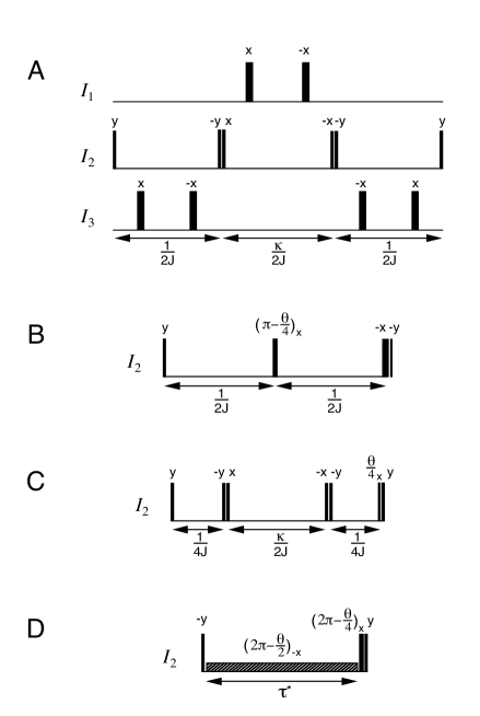
Figure 1: Schematic representation of four basic (narrowband) pulse sequences for the creation of a propagator ${\cal U}_{zzz}(\kappa)=\exp\{-{\rm i}\ \theta\ I_{1z}I_{2z}I_{3z}\}$ with $\theta=2\pi\kappa$. If not explicitely specified otherwise, narrow and wide vertical bars represent spin-selective $\pi/2$ and $\pi$ pulses, respectively. (A) Example of a pulse sequence based on selective decoupling [3, 8, 9], (B) conventional pulse sequence without decoupling [6, 7], (C) improved sequence without decoupling [3], (D) time-optimal geodesic pulse sequence with $\tau^{\ast}=\sqrt{\kappa(4-\kappa)}/2J$ [3].

Figure 8: Transfer efficiency $\eta_{13}(\tau)$ (c.f. Eq. 30) based on broadband versions of sequences, A (dotted curves), C (dashed curves), and D (solid curves). (A) Theoretical curves assuming an ideal spin system (see Fig. 6 top) and ideal rf pulses, (B) simulations based on the coupling constants of [¹⁵N]-acetamide and assuming finite pulse durations and realistic rf inhomogeneity (see text), (C) experimental transfer curves.

References

- [1] R. R. Ernst, G. Bodenhausen, A. Wokaun, Principles of Nuclear Magnetic Resonance in One and Two Dimensions, Clarendon Press, Oxford (1987).
- [2] N. Khaneja, R. W. Brockett, S. J. Glaser, Time Optimal Control in Spin Systems, Phys. Rev. A 63, 03208 (2001).
- [3] N. Khaneja, S. J. Glaser, R. W. Brockett, Sub-Riemannian Geometry and Time Optimal Control of Three Spin Systems: Quantum Gates and Coherence Transfer, Phys. Rev. A, 65, 032301 (2002).
- [4] T. O. Reiss, N. Khaneja, S. J. Glaser, Time-Optimal Coherence-Order-Selective Transfer of In-Phase Coherence in Heteronuclear IS Spin Systems, J. Magn. Reson., 154, 192-195 (2002).
- [5] S. J. Glaser, T. Schulte-Herbrüggen, M. Sieveking, O. Schedletzky, N. C. Nielsen, O. W. Sørensen, C. Griesinger, Unitary Control in Quantum Ensembles, Maximizing Signal Intensity in Coherent Spectroscopy, Science 208, 421-424 (1998).
- [6] O. W. Sørensen, Polarization transfer experiments in high-resolution NMR spectroscopy, Prog. NMR Spectrosc. 21, 503-569 (1989).
- [7] A. Meissner, O. W. Sørensen, -spin -quantum coherences in spin systems employed for E.COSY-type measurement of heteronuclear long-range coupling constants in NMR, Chem. Phys. Lett. 276, 97-102 (1997).
- [8] C. H. Tseng, S. Somaroo, Y. Sharf, E. Knill, R. Laflamme, T. F. Havel, D. G. Cory, Quantum simulation of a three-body interaction Hamiltonian on an NMR quantum computer, Phys. Rev. A, 61, 012302 (2000).
- [9] J. Kim, J.-S. Lee, S. Lee, Implementing unitary operators in quantum computation, Phys. Rev. A, 61, 032312 (2000).
- [10] D. G. Cory, A. F. Fahmy, T. F. Havel, Ensemble quantum computing by NMR spectroscopy, Proc. Natl. Acad. Sci 94, 1634-1639 (1997).
- [11] N. Gershenfeld, I, L. Chuang, Bulk spin-resonance quantum computation, Science 275, 350-356 (1997).
- [12] C. H. Bennet, D. P. DiVinvenzo, Quantum information and computation, Nature 404, 247-255 (2000).
- [13] G. A. Morris, R. Freeman, Selective excitation in Fourier transform nuclear magnetic resonance, J. Magn. Reson. 29, 433-462 (1978).
- [14] M. H. Levitt, R. Freeman, T. Frenkiel, Broadband decoupling in high-resolution nuclear magnetic resonance spectroscopy, in ”Advances in Magnetic Resonance” (J. S. Waugh, Ed.), Vol. 11, pp. 47 - 110, Academic Press, San Diego (1983).
- [15] A. Barenco, C.H. Bennett, R. Cleve, D.P. Divincenzo, N. Margolus, P. Shor, T. Sleator, J. Smolin and H. Weinfurter, Elementary gates for quantum computation, Phys. Rev. A 28 (1996).
- [16] T. Schulte-Herbrüggen, O. W. Sørensen, The Relationship between Ensemble Quantum Computing Logical Gates and NMR Pulse Sequences Engineering Exemplified by the SWAP operation, Conc. Magn. Reson. 12(6), 389-395 (2000).
- [17] N. Linden, H. Barjat, E. Kupče, R. Freeman, How to exchange information between twp coupled nuclear spins: the universal SWAP operation, Chem. Phys. Lett. 307, 198-204 (1999).
- [18] Z. L. Mádi, R. Brüschweiler, R. R. Ernst, One-and two-dimensional ensemble quantum computing in spin Liouville space, J. Chem. Phys. 109, 10603-10611 (1998).
- [19] R. Marx, A. F. Fahmy, J. M. Myers, W. Bermel and S. J. Glaser, Approaching Five-Bit NMR Quantum Computing, Phys. Rev. A, 62, 012310/1-8 (2000).
- [20] S. J. Glaser and J. J. Quant, Homonuclear and heteronuclear Hartmann-Hahn transfer in isotropic liquids, in ”Advances in Magnetic and Optical Resonance” (W. S. Warren, Ed.), Vol. 19, pp. 59 - 252, Academic Press, San Diego (1996).