Fast Non-Adiabatic Two Qubit Gates for the Kane Quantum Computer

Abstract

In this paper we apply the canonical decomposition of two qubit unitaries to find pulse schemes to control the proposed Kane quantum computer. We explicitly find pulse sequences for the CNOT, swap, square root of swap and controlled Z rotations. We analyze the speed and fidelity of these gates, both of which compare favorably to existing schemes. The pulse sequences presented in this paper are theoretically faster, higher fidelity, and simpler. Any two qubit gate may be easily found and implemented using similar pulse sequences. Numerical simulation is used to verify the accuracy of each pulse scheme.

I Introduction

The advent of quantum algorithms Grover (1997); Shor (1997) that can out-perform the best known classical algorithms has inspired many different proposals for a practical quantum computer Knill et al. (2001); Gershenfeld and Chuang (1997); Cory et al. (1997); Cirac and Zoller (1995); Nakamura et al. (1998); Imamoglu et al. (1999); Kane (1998). One of the most promising proposals was presented by Kane Kane (1998). In this proposal a solid state quantum computer based on the nuclear spins of $\mathrm{{}^{31}P}$ atoms was suggested. Although initially difficult to fabricate, this scheme has several advantages over rival schemes Knill et al. (2001); Gershenfeld and Chuang (1997); Cory et al. (1997); Cirac and Zoller (1995); Nakamura et al. (1998); Imamoglu et al. (1999). These include the comparatively long decoherence times of the $\mathrm{{}^{31}P}$ nuclear and electron spins Honig (1954); Gordon and Bowers (1958); Feher and Gere (1959); Feher (1959); Honig and Stupp (1960); Faulkner (1969); Chiba and Hirai (1972); Waugh and Slichter (1988), the similarity to existing $\mathrm{Si}$ fabrication technology, and the ability to scale.

There have been two main proposals for pulse sequences to implement a CNOT gate on the Kane quantum computer. In the initial proposal Kane (1998) an adiabatic CNOT gate was suggested. Since that time the details of this gate have been investigated and optimized Goan and Milburn (2000); Wellard (2001); Wellard and Hollenberg (2001); Fowler et al. (2003). This adiabatic scheme takes a total time of approximately $26\mu s$ and has a systematic error of approximately $5\times 10^{-5}$ Wellard (2001). As good as these results are, non-adiabatic gates have the potential to be faster with higher fidelity and allow advanced techniques such as composite rotations and modified RF pulses Cummins and Jones (2000); Tyco (1983).

Wellard et al. Wellard et al. (2002) proposed a non-adiabatic pulse scheme for the CNOT and swap gates. They present a CNOT gate that takes a total time of approximately $80\mu s$ with an error (as defined later in Eq. (91)) of approximately $4\times 10^{-4}$. Although this gate is non-adiabatic it is slower than its adiabatic counterpart. For the non-adiabatic swap gate a total time was calculated of $192\mu s$.

One of the most useful tools in considering two qubit unitary interactions is the canonical decomposition Kraus and Cirac (2001); Hammerer et al. (2002); Khaneja et al. (2001). This decomposition expresses any two qubit gate as a product of single qubit rotations and a simple interaction content. The interaction content can be expressed using just three parameters. In the limit that single qubit rotations take negligible time (in comparison to the speed of interaction), this decomposition can be used to find optimal schemes Hammerer et al. (2002); Khaneja et al. (2001), and of particular inspiration to this paper is an almost optimal systematic method to construct the CNOT gate Bremner et al. (2002).

It is not possible to apply those optimal schemes Hammerer et al. (2002); Khaneja et al. (2001) directly to the Kane quantum computing architecture. They assume single qubit gates take negligible time in comparison with two qubit interactions, whereas on the Kane architecture, they do not. Secondly, in the proposal for the Kane computer, adjacent nuclei are coupled via the exchange and hyperfine interactions through the electrons, rather than directly, and so we have a four ‘qubit’ system (two electrons and two nuclei) rather than a two qubit system. Although we cannot apply optimal schemes directly, in this paper we use the canonical decomposition to simplify two qubit gate design.

Apart from being simple to design and understand, gates described in this paper have many desirable features. Some features of these gates include:

1. They are simpler, higher fidelity and faster than existing proposals.

2. They do not require sophisticated pulse shapes, such as are envisioned in the adiabatic scheme, to implement.

3. Any two qubit gate can be implemented directly using similar schemes. This allows us to implement gates directly rather than as a series of CNOT gates and single qubit rotations.

This paper is organized as follows. Sec. II gives an overview of the Kane quantum computer architecture and single qubit rotations. Sec. III describes the canonical decomposition as it applies to the Kane quantum computer. Section IV describes pulse schemes for Control Z gates and CNOT gates. Sec. V gives potential pulse schemes for swap and square root of swap gates. Finally, the conclusion, Section VI, summarizes the findings of this paper.

II The Kane Quantum Computer

II.1 The Kane Architecture

A schematic diagram of the Kane quantum computer architecture is shown in Fig. 1. The short description given here follows Goan and Milburn Goan and Milburn (2000). This architecture consists of $\mathrm{{}^{31}P}$ atoms doped in a purified $\mathrm{{}^{28}Si}$ ($I=0$) host. Each P atom has nuclear spin of $I=\frac{1}{2}$. Electrodes placed directly above each P atom are referred to as A-Gates, and those between atoms are referred to as J-Gates. An oxide barrier separates the electrodes from the $\mathrm{P}$ doped $\mathrm{Si}$.

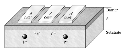
Figure 1: The Kane Quantum Computer Architecture

Each $\mathrm{P}$ atom has five valence electrons. As a first approximation, four of these electrons form covalent bonds to neighboring $\mathrm{Si}$ atoms, with the fifth forming a hydrogen-like S-orbital around each $\mathrm{P^{+}}$ ion. This electron is loosely bound to the $\mathrm{P}$ donor and has a Bohr radius of $a_{B}^{*}\approx 3\mathrm{nm}$, allowing an electron mediated interaction between neighboring nuclei.

In this paper nuclear spin states will be represented by the states $|1\rangle$ and $|0\rangle$. Electronic spin states will be represented by $|\uparrow\rangle$ and $|\downarrow\rangle$. Where electronic states are omitted, it is assumed that they are polarized in the $|\downarrow\rangle$ state. $X$, $Y$ and $Z$ are the Pauli matrices operating on electron and nuclear spins. That is

$$X=\sigma_{x},Y=\sigma_{y},Z=\sigma_{z}.$$ (1)

Operations which may be performed on any system are governed by the Hamiltonian of the system. We now describe the effective spin Hamiltonian for two adjacent qubits of the Kane quantum computer and give a short physical motivation for each term which makes up the overall Hamiltonian:

$$H=\sum_{i=1}^{2}H_{B_{i}}+H_{A_{i}}+H_{J}+H_{ac_{i}}.$$ (2)

where the summation is over each donor atom in the system, $i$.

Under typical operating conditions, a constant magnetic field $B$ will be applied to the entire system, perpendicular to the surface. This contributes Zeeman energies to the Hamiltonian:

$$H_{B}=-g_{n}\mu_{n}BZ_{n}+\mu_{B}BZ_{e}.$$ (3)

A typical value for the Kane quantum computer of $B=2.0\mathrm{T}$ gives Zeeman energy for the electrons of $\mu_{B}B\approx 0.116\mathrm{meV}$, and for the nucleus $g_{n}\mu_{n}B\approx 7.1\times 10^{-5}\mathrm{meV}$.

The hyperfine interaction couples between nuclear and electronic spin. The contribution of the hyperfine interaction to the Hamiltonian is

$$H_{A}=A\sigma_{e}\cdot\sigma_{n},$$ (4)

where strength, $A$, of the hyperfine interaction is proportional to the value of the electron wave-function evaluated at the nucleus,

$$A=\frac{8\pi}{3}\mu_{B}g_{n}\mu_{n}|\psi(0)|^{2}.$$ (5)

A typical strength for the hyperfine interaction is $A=1.2\times 10^{-4}\mathrm{meV}$. Charged A-Gates placed directly above each P nucleus distort the shape of the electronic wavefunction thereby reducing the strength of the hyperfine coupling. The nature of this effect is under numerical investigation Kettle et al. (2003). For the purposes of this paper we have assumed that it will be possible to vary the hyperfine coupling by up to approximately $50\%$.

The exchange interaction couples adjacent electrons. Its contribution to the Hamiltonian is:

$$H_{J}=J\sigma_{e_{1}}\cdot\sigma_{e_{2}},$$ (6)

where $e_{1}$ and $e_{2}$ are two adjacent electrons. The magnitude, $J$, of the exchange interaction depends on the overlap of adjacent electronic wave-functions. J-Gates placed between nuclei distort both electronic wavefunctions to increase or decrease the magnitude of this interaction. A typical value for the exchange energy is $4J=0.124\textrm{meV}$, and for the purposes of this paper we assume that it will be possible to vary the magnitude of the exchange interaction from $J=0$ to $J\approx 0.043\mathrm{meV}$.

A rotating magnetic field, of strength $B_{ac}$ rotating at a frequency of $\omega_{ac}$ can be applied, perpendicular to the constant magnetic field, $B$. The contribution of the rotating magnetic field to the Hamiltonian is:

$$H_{ac} =-g_{n}\mu_{n}B_{ac} \left[X_{n}\cos(\omega_{ac}t)+Y_{n}\sin(\omega_{ac}t)\right]$$ (7)

$$+\mu_{B}B_{ac} \left[X_{e}\cos(\omega_{ac}t)+Y_{e}\sin(\omega_{ac}t)\right],$$

where the strength of the rotating magnetic field is envisioned to be $B_{ac}\approx 0.0025T$.

At an operating temperature of $T=100\mathrm{mK}$, the electrons are almost all polarized by the magnetic field. That is:

$$\frac{n^{\uparrow}_{e}}{n^{\downarrow}_{e}}\approx 2.14\times 10^{-12}.$$ (8)

We assume that electrons are polarized in the $|\downarrow\rangle$ state, and use nuclear spin states as our computational basis.

II.2 Z Rotations

Single qubit rotations are required to implement the two qubit gates described in this paper, as well as being essential for universality. In fact, as we will see they contribute significantly to the overall time and fidelity of each two qubit gate. It is therefore important to consider the time required to implement $Z$, $X$ and $Y$ rotations.

In this subsection we describe how fast Z rotations may be performed varying the voltage on the A-Gates only. A Z rotations is described by the equation:

$$R_{z}(\theta)=e^{i\frac{\theta}{2}Z}.$$ (9)

A Z gate (phase flip), may be implemented as a rotation. It is given up to a global phase by:

$$Z=-iR_{z}\left(\pi\right).$$ (10)

Under the influence of a constant magnetic field, $B$, to second order in $A$ Goan and Milburn (2000), each nuclei will undergo Larmor precession around the Z axis, at frequency of

$$\hbar\omega_{l}=2g_{n}\mu_{n}B+2A+\frac{2A^{2}}{\mu_{B}B+g_{n}\mu_{n}B}.$$ (11)

Z rotations may be performed by variation of the hyperfine interaction from $A$ to $A_{z}$ giving a difference in rotation frequency of

$$\hbar\omega_{z}=2(A-A_{z})+\frac{2(A^{2}-A_{z}^{2})}{\mu_{B}B+g_{n}\mu_{n}B}.$$ (12)

Perturbing the hyperfine interaction for one of the atoms, and allowing free evolution will rotate this atom with respect to the rotation of the unperturbed atoms. The speed of single atom Z rotations depends how much it is possible to vary the strength of the hyperfine interaction, $A$. For numerical simulation we use the typical values shown in Table 1.

Description	Term	Value
Unperturbed Hyperfine Interaction	$A$	$0.1211\times 10^{-3}\textrm{meV}$
Hyperfine Interaction During Z Rotation	$A_{z}$	$0.0606\times 10^{-3}\textrm{meV}$

Table 1: Typical Parameters for a Z Rotation

Under these conditions a Z gate may be performed on a single nuclear spin in approximately

$$t_{Z}\approx 0.021\mathrm{\mu s}.$$ (13)

These rotations occur in a rotating frame, that precesses around the Z axis with a frequency equal to the Larmor frequency. We may have to allow a small time of free evolution until nuclei that are not affected by the Z rotation orientate themselves to their original phase. The time required for this operation is less than

$$t_{F}\leq 0.02\mathrm{\mu s}$$ (14)

II.3 X and Y Rotations

In this section we show how techniques, similar to those used in NMR Becker (2000); Slichter (1990); Goan and Milburn (2000), may be used to implement X and Y rotations. X and Y rotations are described by the equations:

$$R_{x}(\theta) = e^{i\frac{\theta}{2}X},$$ (15)

$$R_{y}(\theta) = e^{i\frac{\theta}{2}Y}.$$ (16)

X and Y rotations are performed by application of a rotating magnetic field, $B_{ac}$. The rotating magnetic field is resonant with the Larmor precession frequency given in Eq. (11), that is:

$$\omega_{ac}=\omega_{l}.$$ (17)

In contrast to NMR, in the Kane proposal we have direct control over the Larmor frequency of each individual $\mathrm{P}$ nucleus. By reducing the hyperfine coupling for the atom we wish to target from $A$ to $A_{x}$ we may apply an oscillating magnetic field that is only resonant with the Larmor frequency of only one of the atoms. This allows us to induce an X or Y rotation on an individual atom. To the first order, the frequency of this rotation may be approximated by:

$$\hbar\omega_{x}=g_{n}\mu_{n}B_{ac}\left(1+\frac{A_{x}}{g_{n}\mu_{n}B}\right).$$ (18)

The speed of an X rotation is directly proportional to the strength of the rotating magnetic field, $B_{ac}$. As the strength of the rotating magnetic field, $B_{ac}$ increases, the fidelity of the operation decreases. The reason is that in frequency space the Full Width Half Maximum (FWHM) of the transition excited by the rotating magnetic field increases in proportional to $B_{ac}$. That is, as $B_{ac}$ increases we begin to excite non-resonant transitions. The larger separation, in frequency space, between Larmor frequencies, the smaller this systematic error. Since the Larmor precession frequency depends on how much we are able to vary the hyperfine interaction, $A$, it determines how strong we are able to make $B_{ac}$

For the purpose of simulation, the typical values shown in Table 2 for the unperturbed hyperfine interaction strength $A$, the hyperfine interaction strength during the X rotation $A_{x}$, applied magnetic field strength $B$, and rotating magnetic field strength $B_{ac}$ were used.

Description	Term	Value
Unperturbed Hyperfine Interaction	$A$	$0.1211\times 10^{-3}\textrm{meV}$
Hyperfine Interaction during X Rotation	$A_{x}$	$0.0606\times 10^{-3}\textrm{meV}$
Constant Magnetic Field Strength	$B$	$2.000\textrm{T}$
Rotating Magnetic Field Strength	$B_{ac}$	$0.0025\textrm{T}$

Table 2: Typical Parameters for an X Rotation

Using these parameters this gives the overall time to perform an X gate on a single qubit in approximately:

$$t_{X}\approx 6.4\mu s.\\$$ (19)

Any single qubit gate may be expressed as a product of X, Y and Z rotations. Ideally, X and Y rotations should be minimized because Z rotations may be performed much faster than X or Y rotations. For example, a Hadamard gate may be expressed as a product of Z and X rotations:

$$H=R_{z}\!\left(\frac{\pi}{2}\right)\ R_{x}\!\left(\frac{\pi}{2}\right)\ R_{z}\!\left(\frac{\pi}{2}\right).$$ (20)

Thus, from the above discussion, Hadamard gate takes a time of approximately:

$$t_{H}\approx 3.2\mu s.\\$$ (21)

II.4 Nuclear Spin Interaction

In this section we show the results of second order perturbation theory to describe the interaction between two neighboring $P$ atoms. This interaction between nuclei is coupled by electron interactions. We consider the case where the hyperfine couplings, between each nucleus and its electron are equal, that is:

$$A=A_{1}=A_{2}.$$ (22)

We allow coupling between electrons, that is:

$$J>0,$$ (23)

but restrict ourselves to be far from an electronic energy level crossing,

$$J\ll\frac{\mu_{B}B}{2}.$$ (24)

Under these conditions electrons will remain in the polarized $|\downarrow\downarrow\rangle$ ground state.

In this situation analysis has been performed using second order perturbation theory Goan and Milburn (2000). To second order in $A$, the energy levels are:

$$E_{|11\rangle} = -2\mu_{B}B+J+2g_{n}\mu_{n}B+2A,$$ (25)

$$E_{|s_{n}\rangle} = -2\mu_{B}B+J-\frac{2A^{2}}{\mu_{B}B+g_{n}\mu_{n}B},$$ (26)

$$E_{|a_{n}\rangle} = -2\mu_{B}B+J-\frac{2A^{2}}{\mu_{B}B+g_{n}\mu_{n}B-2J},$$ (27)

$$E_{|00\rangle} = -2\mu_{B}B+J-2g_{n}\mu_{n}B-2A$$ (28)

$$\!-\frac{2A^{2}}{\mu_{B}B+g_{n}\mu_{n}B-2J}-\frac{2A^{2}}{\mu_{B}B+g_{n}\mu_{n}B},\quad$$

where the symmetric $|s_{n}\rangle$ and anti-symmetric $|a_{n}\rangle$ energy eigenstates are given by:

$$|s_{n}\rangle = \frac{1}{\sqrt{2}}\left(|10\rangle+|01\rangle\right),$$ (29)

$$|a_{n}\rangle = \frac{1}{\sqrt{2}}\left(|10\rangle-|01\rangle\right).$$ (30)

Notice that the energies are symmetric around

$$E_{0} =-2\mu_{B}B +J-\frac{A^{2}}{\mu_{B}B+g_{n}\mu_{n}B-2J}$$ (31)

$$-\frac{A^{2}}{\mu_{B}B+g_{n}\mu_{n}B}.$$

Since we are free to choose our zero point energy to be $E_{0}$ (or equivalently ignore a global phase of a wavefunction, $|\psi\rangle$) we may rewrite the second order approximation as:

$$E_{|\downarrow\downarrow\rangle|11\rangle}= \hbar\omega_{B},$$ (32)

$$E_{|\downarrow\downarrow\rangle|s_{n}\rangle}= \hbar\omega_{S},$$ (33)

$$E_{|\downarrow\downarrow\rangle|a_{n}\rangle}= - \hbar\omega_{S},$$ (34)

$$E_{|\downarrow\downarrow\rangle|00\rangle}= - \hbar\omega_{B},$$ (35)

where $\omega_{B}$ and $\omega_{S}$ are given by:

$$\hbar\omega_{B} = 2A+2g_{n}\mu_{n}B+$$ (36)

$$\frac{A^{2}}{\mu_{B}B+g_{n}\mu_{n}B}+\frac{A^{2}}{\mu_{B}B+g_{n}\mu_{n}B-2J},$$

$$\hbar\omega_{S} = \frac{A^{2}}{\mu_{B}B+g_{n}\mu_{n}B-2J}-\frac{A^{2}}{\mu_{B}B+g_{n}\mu_{n}B}.$$ (37)

The reason for this representation of the energy will become clear in the next section. Typical values were used during numerical simulation of the interaction between nuclei are shown in Table 3.

Description	Term	Value
Hyperfine Interaction during Interaction	$A_{U}$	$0.1197\times 10^{-3}\ \textrm{meV}$
Exchange Interaction during Interaction	$J_{U}$	$0.0423\ \textrm{meV}$

Table 3: Typical Parameters during Interaction

III The Canonical Decomposition

In this section we describe the canonical decomposition, and describe how this decomposition may be applied to the Kane quantum computer.

III.1 Mathematical Description of Canonical Decomposition

The canonical decomposition Kraus and Cirac (2001); Khaneja et al. (2001) decomposes any two qubit unitary operator into a product of four single qubit unitaries and one entangling unitary.

$$U=(V_{1}\otimes V_{2})\ U_{can}\ (W_{1}\otimes W_{2}).$$ (38)

where $V_{1}$, $V_{2}$, $W_{1}$ and $W_{2}$ are single qubit unitaries, and $U_{can}$ is the two qubit interaction. The symbol $\otimes$ represents the tensor product of two matrices.

$U_{can}$ has a simple form involving only three parameters, $\alpha_{x}$, $\alpha_{y}$ and $\alpha_{z}$:

$$U_{can}=e^{i\alpha_{x}X\otimes X}\ e^{i\alpha_{y}Y\otimes Y}\ e^{i\alpha_{z}Z\otimes Z}.$$ (39)

This purely non-local term is known as the interaction content of the gate. It is not difficult to show that each of the terms in the interaction content, $e^{i\alpha_{x}X\otimes X}$, $e^{i\alpha_{y}Y\otimes Y}$ and $e^{i\alpha_{z}Z\otimes Z}$, commute with each other.

Physically each of the terms $e^{i\alpha_{x}X\otimes X}$, $e^{i\alpha_{y}Y\otimes Y}$, and $e^{i\alpha_{z}Z\otimes Z}$ correspond to a type of controlled rotation. For example, following Ref. Bremner et al. (2002)

$$e^{i\alpha_{z}Z\otimes Z}$$ (40)

$$= \cos{\alpha_{z}}I\otimes I+i\sin{\alpha_{z}}Z\otimes Z$$

$$= \cos{\alpha_{z}}(|0\rangle\langle 0|+|1\rangle\langle 1|)\otimes I$$

$$+i\sin{\alpha_{z}}(|0\rangle\langle 0|-|1\rangle\langle 1|)\otimes Z$$

$$= |0\rangle\langle 0|\otimes e^{i\alpha_{z}Z}+|1\rangle\langle 1|\otimes e^{-i\alpha_{z}Z}$$

$$= \left(I\otimes e^{i\alpha_{z}Z}\right)\ \left(|0\rangle\langle 0|\otimes I\ +\ |1\rangle\langle 1|\otimes e^{-i2\alpha_{z}Z}\right).$$

This shows that up to a single qubit rotation, $e^{i\alpha_{z}Z\otimes Z}$ is equivalent to a controlled Z rotation. This holds true for the other two terms. If we denote the eigenstates of X by

$$X|x_{+}\rangle = +|x_{+}\rangle,$$ (41)

$$X|x_{-}\rangle = -|x_{-}\rangle,$$ (42)

then a similar analysis shows that

$$\left(I\otimes e^{-i\alpha_{x}X}\right)e^{i\alpha_{x}X\otimes X}$$

$$=|x_{+}\rangle\langle x_{+}|\otimes I\ +\ |x_{-}\rangle\langle x_{-}|\otimes e^{-i2\alpha_{x}X},$$ (43)

and that

$$\left(I\otimes e^{-i\alpha_{y}Y}\right)e^{i\alpha_{y}Y\otimes Y}$$

$$=|y_{+}\rangle\langle y_{+}|\otimes I\ +\ |y_{-}\rangle\langle y_{-}|\otimes e^{-i2\alpha_{y}Y}.$$ (44)

These operations are equivalent to controlled rotations in the $X$ and $Y$ directions respectively. For the first case, if the control qubit is in the $|x_{-}\rangle$ state an X rotation is applied to the target qubit, and not applied if the control qubit is in the $|x_{+}\rangle$ state. Similarly for Y.

Single qubit rotations, $V_{1},V_{2},W_{1},W_{2}$ are possible on the Kane quantum computing architecture, the remaining task is to specify the pulse sequence for the purely entangling unitary $U_{can}$. Fortunately this is always possible, as any interaction (with single qubit rotations) between the two nuclei is sufficient Dodd et al. (2002). In fact, it is a relatively simple task to use almost any interaction between qubits to generate any desired operation.

III.2 Calculation of the Interaction Content between Nuclei

In this subsection we will see how it is possible to apply the canonical decomposition to the Kane quantum computer. This is important as this natural interaction of the system will be manipulated by single qubit unitaries to find the pulse scheme of any two qubit gate. The canonical decomposition provides a unique way of looking at this interaction.

The interaction we will apply the canonical decomposition to is free evolution of the configuration described in Sec. II.4, using the results cited there from second order perturbation theory. After a particular time of free evolution, our system will have evolved according to unitary dynamics, which we may decompose using the canonical decomposition:

$$U_{sys}=(V_{1}^{s}\otimes V_{2}^{s})\ U_{can}^{s}\ (W_{1}^{s}\otimes W_{2}^{s}),$$ (45)

where the super-script ‘s’ indicates a physical operation present in our system.

We wish to find the interaction content $U_{can}^{s}$ of this free evolution. Systematic methods for doing this are given in Kraus and Cirac (2001); Haselgrove (2002); Hammerer et al. (2002). This is most easily done by noting any interaction content, $U_{can}$ is diagonal in the so-called magic basis, otherwise known as the Bell basis. This basis is:

$$|\Phi_{1}\rangle = \frac{1}{\sqrt{2}}(|00\rangle+|11\rangle),$$ (46)

$$|\Phi_{2}\rangle = \frac{-i}{\sqrt{2}}(|00\rangle-|11\rangle),$$ (47)

$$|\Phi_{3}\rangle = \frac{1}{\sqrt{2}}(|01\rangle-|10\rangle),$$ (48)

$$|\Phi_{4}\rangle = \frac{-i}{\sqrt{2}}(|01\rangle+|10\rangle).$$ (49)

$\alpha_{x}$, $\alpha_{y}$ and $\alpha_{z}$ are related to the eigenvalues $e^{i\lambda_{1}}$, $e^{i\lambda_{2}}$, $e^{i\lambda_{3}}$ and $e^{i\lambda_{4}}$ of $U_{can}$. That is:

$$\lambda_{1} = +\alpha_{x}-\alpha_{y}+\alpha_{z},$$ (50)

$$\lambda_{2} = -\alpha_{x}+\alpha_{y}+\alpha_{z},$$ (51)

$$\lambda_{3} = -\alpha_{x}-\alpha_{y}-\alpha_{z},$$ (52)

$$\lambda_{4} = +\alpha_{x}+\alpha_{y}+\alpha_{z}.$$ (53)

It is possible to relate these eigenvalues to our system. After a time $t$, each of the eigenstates of the system will have evolved according the Schrödinger equation, which we may view as having performed an operation $U_{sys}(t)$ on the system. As we showed in Sec. II.4:

$$U_{sys}|11\rangle = e^{+i\theta_{B}}|11\rangle,$$ (54)

$$U_{sys}|00\rangle = e^{-i\theta_{B}}|00\rangle,$$ (55)

$$U_{sys}|s\rangle = e^{+i\theta_{S}}|s\rangle,$$ (56)

$$U_{sys}|a\rangle = e^{-i\theta_{S}}|a\rangle,$$ (57)

where

$$\theta_{S} = \omega_{S}t,$$ (58)

$$\theta_{B} = \omega_{B}t.$$ (59)

Applying Eqs. (54) – (57) to Eqs. (46) – (49), we obtain:

$$U_{sys}|\Phi_{1}\rangle = \cos(\theta_{B})|\Phi_{1}\rangle-\sin(\theta_{B})|\Phi_{2}\rangle,$$ (60)

$$U_{sys}|\Phi_{2}\rangle = \cos(\theta_{B})|\Phi_{2}\rangle+\sin(\theta_{B})|\Phi_{1}\rangle,$$ (61)

$$U_{sys}|\Phi_{3}\rangle = e^{-i\theta_{S}}|\Phi_{3}\rangle,$$ (62)

$$U_{sys}|\Phi_{4}\rangle = e^{+i\theta_{S}}|\Phi_{4}\rangle.$$ (63)

This shows that in the magic basis, $U_{sys}$ is given by:

$$U_{sys}=\left[\begin{array}[]{cccc}\cos(\theta_{B})&\sin(\theta_{B})&0&0\\ -\sin(\theta_{B})&\cos(\theta_{B})&0&0\\ 0&0&e^{-i\theta_{S}}&0\\ 0&0&0&e^{i\theta_{S}}\\ \end{array}\right].$$ (64)

It is possible to find the eigenvalues $\lambda_{1}$, $\lambda_{2}$, $\lambda_{3}$ and $\lambda_{4}$. We note that the eigenvalues of $U^{T}U$ in the magic basis are given by

$$\lambda(U^{T}U)=\{e^{2i\lambda_{1}},e^{2i\lambda_{2}},e^{2i\lambda_{3}},e^{2i\lambda_{4}}\}.$$ (65)

Calculation of the eigenvalues of $U_{sys}^{T}U_{sys}$ is easy since $U_{sys}^{T}U_{sys}$ is already diagonal in this basis, with diagonal elements being $\{1,1,e^{-2i\theta_{S}},e^{2i\theta_{S}}\}$. Care must be exercised at this point, because it is not clear which branch should be used when taking the argument. In our case, as long as $0\leq\theta_{S}\leq\frac{\pi}{2}$ Haselgrove (2002) then

$$\lambda_{1} = 0,$$ (66)

$$\lambda_{2} = 0,$$ (67)

$$\lambda_{3} = -\theta_{S},$$ (68)

$$\lambda_{4} = +\theta_{S}.$$ (69)

Using Eqs. (50) – (53) we may solve for the coefficients $\alpha_{x}$, $\alpha_{y}$ and $\alpha_{z}$, giving:

$$\alpha_{x}^{s} = \frac{1}{2}\theta_{S},$$ (70)

$$\alpha_{y}^{s} = \frac{1}{2}\theta_{S},$$ (71)

$$\alpha_{z}^{s} = 0.$$ (72)

Single qubit rotations, $W_{1}^{s},W_{2}^{s},V_{1}^{s},V_{2}^{s}$, induced are Z rotations. Z rotations are fast, and may be canceled in comparatively little time by single qubit Z rotations in the opposite direction:

$$(V_{1}^{s\dagger}\otimes V_{2}^{s\dagger})\ U_{sys}\ (W_{1}^{s\dagger}\otimes W_{2}^{s\dagger})=U_{can}^{s}.$$ (73)

For notational convenience we will now label the interaction content of the system by an angle rather than by its time. The time for this interaction may be calculated through Eqs. (70) – (72), (58) and (37). Therefore, we write:

$$U_{can}^{s}(\phi)=e^{i\phi X\otimes X+i\phi Y\otimes Y},$$ (74)

where

$$\phi=\frac{1}{2}\theta_{S}.$$ (75)

This analysis has been based on second order perturbation theory. As we approach the electronic energy level crossing, this approach is no longer valid. Close to this crossing numerical analysis shows the eigenvalues are no longer symmetric which implies $\alpha_{z}^{s}$ becomes non-zero. Unfortunately in this regime, we excite the system into higher energy electronic configurations.

Given any two qubit gate, such as the CNOT gate, there are many different possible choices of single qubit rotations and free evolution that will implement a desired gate. Z rotations are faster single qubit rotations than X and Y rotations, and therefore it is desirable to minimize X and Y rotations in order to optimize the time required, for any given two qubit gate.

IV The CNOT and Controlled Z Gates

IV.1 Introduction

The CNOT gate is a particularly often cited example of a two qubit gate. CNOT and single qubit rotations are universal for quantum computation DiVincenzo (1995). Many implementations, including the Kane proposal Kane (1998), use this fact to demonstrate that they can, in principle, perform any quantum algorithm. It is a member of the so-called fault tolerant Shor (1996) set of gates, which are universal for quantum computing, and are particularly important in error correction. In this section we find a pulse scheme to implement the CNOT gate on the Kane quantum computer.

Controlled Z rotations, sometimes known as controlled phase gates, are some of the most important operations for implementing quantum algorithms. In particular, one of the simplest ways to implement quantum Fourier transformations (QFTs) uses multiple controlled Z rotations (see for example Nielsen and Chuang (2001)). Single qubit rotations and the controlled Z gate are, like the CNOT gate, universal for quantum computation. Controlled Z rotations may be used in the construction of controlled X and Y rotations. In this section we find a pulse scheme to implement any controlled Z rotation on the Kane quantum computer.

Because these two gates have similar interaction contents we consider them together. We will first show how to construct a controlled Z gate of any angle, and use this gate directly to construct a CNOT gate.

A controlled Z rotation of angle $\theta$ is defined in the computational basis by

$$U_{\Lambda Z}(\theta)=\left[\begin{array}[]{cccc}1&0&0&0\\ 0&1&0&0\\ 0&0&1&0\\ 0&0&0&e^{i\theta}\end{array}\right].$$ (76)

The canonical decomposition of the controlled Z rotation by an angle $\theta$ has an interaction content consisting of:

$$\alpha_{x} = 0,$$ (77)

$$\alpha_{y} = 0,$$ (78)

$$\alpha_{z} = \frac{\theta}{2}.$$ (79)

This interaction content may be found by using systematic methods Kraus and Cirac (2001); Haselgrove (2002); Hammerer et al. (2002). The controlled Z gate also requires a Z rotation as described by Eq. (40).

CNOT is defined in the computational basis by the matrix

$$U_{CNOT}=\left[\begin{array}[]{cccc}1&0&0&0\\ 0&1&0&0\\ 0&0&0&1\\ 0&0&1&0\end{array}\right].$$ (80)

The canonical decomposition of CNOT has an interaction content with angles of

$$\alpha_{x} = 0,$$ (81)

$$\alpha_{y} = 0,$$ (82)

$$\alpha_{z} = \frac{\pi}{4}.$$ (83)

Since the CNOT and Controlled Z gates are both types of controlled rotation similar to those described in Sec. III.1, it is not a surprise that they have a similar interaction content. In fact, Control Z gates (that is, a controlled Z rotation by an angle of $\pi$) and CNOT gates have an identical interaction content, and are therefore equivalent up to single qubit rotations. A CNOT gate may be constructed from a Control Z gate conjugated by $I\otimes H$.

IV.2 The Construction

Our first task in finding a suitable pulse scheme for the controlled Z rotation to find a pulse scheme which implements the interaction content [Eqs. (77) – (79)] of the controlled Z rotation. Techniques have direct analogues in NMR Becker (2000); Slichter (1990).

The first technique Bremner et al. (2002) is to conjugate by $I\otimes X$, $I\otimes Y$, or $I\otimes Z$ to change the sign of two of these parameters. For example:

$$(I\otimes Z) e^{i\alpha_{x}X\otimes X+i\alpha_{y}Y\otimes Y+i\alpha_{z}Z\otimes Z} (I\otimes Z)$$

$$= e^{-i\alpha_{x}X\otimes X-i\alpha_{y}Y\otimes Y+i\alpha_{z}Z\otimes Z}.$$ (84)

This can be useful, because it allows us to exactly cancel every controlled rotation except one:

$$(I\otimes Z)\ U_{can}\ (I\otimes Z)\ U_{can}=e^{i2\alpha_{z}Z\otimes Z}.$$ (85)

In our case, however, it turns out that $\alpha_{z}^{s}=0$. In order to reorder the parameters a useful technique is to conjugate by Hadamards Bremner et al. (2002). This is one of only several choices of single qubit rotations which reorder the parameters. In this case the order of the parameters is:

$$(H\otimes H)\ e^{i\alpha_{x}X\otimes X+i\alpha_{y}Y\otimes Y+i\alpha_{z}Z\otimes Z}\ (H\otimes H)$$

$$=e^{i\alpha_{z}X\otimes X+i\alpha_{y}Y\otimes Y+i\alpha_{x}Z\otimes Z}.$$ (86)

Combining these two techniques gives the following construction

$$e^{i\theta Z\otimes Z}$$ (87)

$$= (Z\otimes I)\ (H\otimes H)\ U_{can}^{s}\left(\frac{\theta}{2}\right)\ (H\otimes H)\ (Z\otimes I)$$

$$\quad(H\otimes H)\ U_{can}^{s}\left(\frac{\theta}{2}\right)\ (H\otimes H).$$

To find the final construction, several one qubit optimizations were made by combining adjacent single qubit rotations and using the identities:

$$HZH = X,$$ (88)

$$HH = I.$$ (89)

Operations may be performed in parallel. For example, performing identical X or Y rotations on separate nuclei is a natural operation of the system, because magnetic fields are applied globally. Performing operations in parallel is faster, and also higher fidelity than performing them one at a time.

The construction of the controlled Z rotation is shown in Fig. 2. In this circuit the single qubit rotations specified in Eq. (40) have been included. The period of interaction between nuclei may be increased or decreased to produce controlled rotations by any angle, $\theta$, as specified in Eqs. (87), (74), (58) and (37).

Figure 2: Circuit Diagram for Controlled Z Pulse Sequence

Our task of constructing a CNOT is now comparatively simple. We note that a CNOT gate has the same interaction term as the controlled Z (controlled phase) operation. These gates are therefore equivalent up to local operations.

Conjugation by $I\otimes H$ will turn a controlled Z operation into a CNOT gate. Using some simple one qubit identities to simplify the rotations at the beginning and end of the pulse sequences we arrive at the decomposition illustrated in the circuit diagram shown in Fig. 3.

Figure 3: Circuit diagram for CNOT pulse sequence

IV.3 Time and Fidelity

Throughout the paper we define fidelity as

$$F(|\psi\rangle,|\psi_{0}\rangle)=|\langle\psi|\psi_{0}\rangle|^{2},$$ (90)

with $|\psi\rangle$ being the actual state obtained from evolution, and $|\psi_{0}\rangle$ being the state which is desired. We define the error in terms of the fidelity as

$$E=\max_{|\psi\rangle}\left[1-F(|\psi\rangle,|\psi_{0}\rangle)\right].$$ (91)

where the maximumization is performed over the output of all the computational basis states, $|\psi\rangle$.

Numerical simulations were carried out by numerically integrating Schrodinger’s equation for the Hamiltonian of the system, Eq. (2). The results of this numerical simulation for the pulse sequence of the CNOT gate are shown in Fig. 4. These graphs show each of the states and the transitions which are made. In these figures it is possible to see the evolution of each of the four computational basis states. The control qubit is the second qubit and the target qubit is the first qubit.

(a) $|00\rangle$ initial state

(b) $|01\rangle$ initial state

(c) $|10\rangle$ initial state

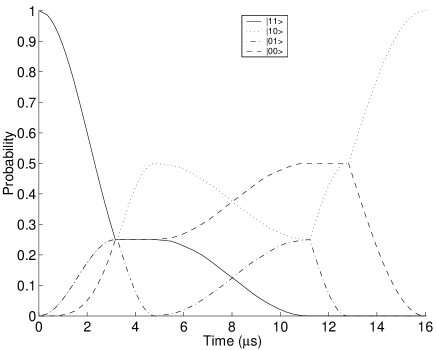
(d) $|11\rangle$ initial state

Figure 4: Numerical simulation of the CNOT gate showing different initial conditions

According to the numerical results, a full Controlled Z gate takes a total time of $16.1\mu s$ and has an error of approximately $4\times 10^{-5}$. Similarly we find the CNOT gate takes a total time of $16.0\mathrm{\mu s}$. The time required for this gate can be grouped as shown in Table 4.

Description	Time
X rotations	12.6 $\mathrm{\mu s}$
Z rotations	0.2 $\mathrm{\mu s}$
2 qubit interaction	3.2 $\mathrm{\mu s}$
Total	16.0 $\mathrm{\mu s}$

Table 4: Time for CNOT Gate

$X$ and $Y$ rotations make up the majority of the time taken to implement the controlled Z and CNOT gates. In the CNOT gate, only $3.2\mathrm{\mu s}$ is spent implementing the entangling part of the gate, whereas $12.6\mathrm{\mu s}$ is required to implement the $X$ and $Y$ rotations.

We can see via simulation that the systematic error in the CNOT gate is approximately $4\times 10^{-5}$. Some of this error will be due to errors during simulation, and breakdown of the second order approximation. A large part of the error, particularly if the hyperfine interaction may not be varied very much, is due to X rotations where unintended non-resonant transitions are excited along with the intended rotation.

V The Swap and Square Root of Swap Gates

V.1 Introduction

Figure 5: Circuit Diagram for the Swap gate pulse sequence

Figure 6: The Circuit Diagram for the Square Root of Swap Pulse Sequence

One of the most important gates for the Kane quantum computer is envisioned to be the swap gate. This is because, in the Kane proposal, only nearest neighbor interactions are allowed. This gate swaps the quantum state of two qubits. By using the swap gate it is possible to swap qubits until they are nearest neighbors, interact them, and then swap them back again. Having an efficient method to interact qubits which are not adjacent to each other is therefore important, and the swap gate, with its high level of information transfer, is one possible method of achieving this.

The square root of swap gate has been suggested for the quantum dot spin based quantum computer architecture Loss and DiVincenzo (1998), where it is a particularly natural operation. In our system it is not such a natural operation, but that does not mean that we cannot construct it. Like the CNOT gate, the square root of swap (together with single qubit rotations) is universal for quantum computation. In this section we find a pulse sequence to implement both the swap and the square root of swap gates on the Kane quantum computer architecture.

The swap gate is defined in the computational basis by:

$$U_{Swap}=\left[\begin{array}[]{cccc}1&0&0&0\\ 0&0&1&0\\ 0&1&0&0\\ 0&0&0&1\end{array}\right]$$ (92)

The canonical decomposition of the swap gate has an interaction content with angles of:

$$\alpha_{x} = \frac{\pi}{4}$$ (93)

$$\alpha_{y} = \frac{\pi}{4}$$ (94)

$$\alpha_{z} = \frac{\pi}{4}$$ (95)

The square root of swap gate is defined in the computational basis by:

$$U_{SS}=\left[\begin{array}[]{cccc}1&0&0&0\\ 0&\frac{1}{2}(1+i)&\frac{1}{2}(1-i)&0\\ 0&\frac{1}{2}(1-i)&\frac{1}{2}(1+i)&0\\ 0&0&0&1\end{array}\right]$$ (96)

The canonical decomposition of the square root of swap gate has an interaction term consisting of:

$$\alpha_{x} = -\frac{\pi}{8},$$ (97)

$$\alpha_{y} = -\frac{\pi}{8},$$ (98)

$$\alpha_{z} = -\frac{\pi}{8}.$$ (99)

Since the square root of swap and swap gates have essentially the same interaction content, their constructions are very similar, and are therefore considered together here.

V.2 The Construction

The easiest way to construct a swap gate is simply to use free evolution to obtain the angles $\alpha_{x}$ and $\alpha_{y}$ which is natural for our system. The only remaining term is the $\alpha_{z}$ term, which for our system will naturally be 0. We may obtain this term by applying a pulse sequence similar to the Controlled Z rotation as described in Sec. IV. The resulting construction swap gate is shown in the diagram in Fig. 5.

The interaction content of the square root of swap gate is exactly half that of the swap gate, and it is negative. We use exactly the same technique used to obtain the swap gate, only allowing the nuclei to interact for exactly half the time. To make the terms negative we conjugate by $Z\otimes I$. The construction of the square root of swap gate obtained using this method is shown in Fig. 6.

V.3 Speed and Fidelity

The swap and square root of swap gates were simulated numerically. The resulting transitions for the swap gate are shown in Fig. 7. Similar results were obtained for the square root of swap gate, not shown here.

(a) $|00\rangle$ initial state

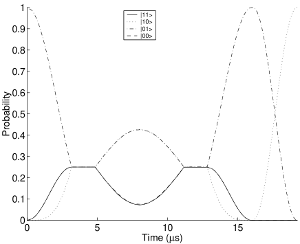
(b) $|01\rangle$ initial state

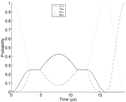
(c) $|10\rangle$ initial state

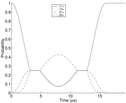
(d) $|11\rangle$ initial state

Figure 7: Numerical Simulation of the Swap Gate

The swap gate takes a total time of $19.2\mu s$, and has a fidelity of approximately $7\times 10^{-5}$. The majority of time in this gate is taken by X and Y rotations, which are also the major source of error.

This is substantially faster than an existing suggestion for the swap gate Wellard (2001) of $192\mu s$. It is also faster than using three adiabatic CNOT gates, which would take approximately $78\mu s$.

According to numerical simulation the square root of swap gate takes $16.8\mu s$ and has an error of approximately $5\times 10^{-5}$. This is the first explicit proposal for the Kane quantum computer for the square root of swap gate.

The square root of swap gate has been suggested in the context of quantum computation for quantum dots Loss and DiVincenzo (1998). It is universal for quantum computation and therefore can be used to construct a CNOT gate. Unfortunately in this case, a CNOT constructed from the square root of swap gate presented here would take approximately $40\mu s$ which is much longer than the pulse sequence presented in this paper for the CNOT gate.

VI Conclusion

We have shown how the canonical decomposition may be applied to the Kane quantum computer. We found the canonical decomposition of a natural operation of the computer, that is, free evolution with hyperfine interactions equal and the exchange interaction non-zero. We then used this interaction to form two qubit gates which may be applied to the Kane quantum computer. These gates and their times and fidelities are shown in Table 5.

Gate	Time	Error
CNOT	$16.0\mu s$	$4\times 10^{-5}$
Swap	$19.2\mu s$	$7\times 10^{-5}$
Square Root of Swap	$16.2\mu s$	$5\times 10^{-5}$
Controlled Z	$16.1\mu s$	$4\times 10^{-5}$

Table 5: Gate Times and Fidelities

The majority of the time required to implement each of these two qubit gates is used to implement single qubit rotations. Were we able to perform these rotations faster and more accurately then the gates presented here would also benefit. Another possible avenue of research is to investigate the effect of decoherence on the system.

To our knowledge this is the fastest proposal for swap, square root of swap, CNOT and controlled Z operations on the Kane quantum computer architecture. We have shown how a representative set of two qubit gates may be implemented on the Kane quantum computer. These methods may prove particularly powerful because they only involve characterization by three parameters which may be determined theoretically, as shown here, or through experiment. Once determined, these parameters may be used to construct any two qubit gate.