Measurement of one-photon and two-photon wavepackets
in spontaneous parametric down-conversion

Abstract

One-photon and two-photon wavepackets of entangled two-photon states in spontaneous parametric down-conversion (SPDC) fields are calculated and measured experimentally. For type-II SPDC, measured one-photon and two-photon wavepackets agree well with theory. For type-I SPDC, the measured one-photon wavepacket agree with the theory. However, the two-photon wavepacket is much bigger than the expected value and the visibility of interference is low. We identify the sources of this discrepancy as the spatial filtering of the two-photon bandwidth and non-pair detection events caused by the detector apertures and the tuning curve characteristics of the type-I SPDC.

I Introduction

The two-photon state generated via spontaneous parametric down-conversion (SPDC) is one of the most well-known examples of two-particle entangled states. The SPDC process can be briefly explained as a spontaneous splitting or decay of a pump photon into a pair of daughter photons (typically called signal and idler photons) in a nonlinear optical crystal klyshko . This spontaneous decay or splitting only occurs when energies and momentum of the interacting photons satisfy the conservation condition, which is known as the phase matching condition. Signal and idler photons have the same polarization in type-I phase matching and have orthogonal polarization in type-II phase matching.

If the phase matching is perfect, assuming monochromatic plane wave pump, it is not hard to see that the state of SPDC should be written as

$$|\Psi\rangle = \sum_{s,i}\delta(\omega_{s}+\omega_{i}-\omega_{p})\delta(\mathbf{k}_{s}+\mathbf{k}_{i}-\mathbf{k}_{p})$$ (1)

$$\times a_{s}^{\dagger}(\omega(\mathbf{k}_{s}))a_{i}^{\dagger}(\omega_{i}(\mathbf{k}_{i}))|0\rangle,$$

where $\omega_{j}$, $\mathbf{k}_{j}$ ($j=s,i,p$) are the frequency and the wave vectors of the signal, idler, and the pump, respectively, and $a_{s}^{\dagger}(\omega(\mathbf{k}_{s}))$ is the creation operator for the signal photon. The $\delta$ functions in state (1) ensure that the signal and the idler photons satisfy the phase matching condition, i.e., there is only one energy or wave vector for the idler photon corresponding to a given energy or wave vector for the signal photon. In other words, the signal-idler photon pair is perfectly entangled in energy and momentum. Such a perfectly entangled two-photon state (in energy and momentum) naturaly has an infinite two-photon coherence time.

In reality, such a strict one-to-one correspondence does not happen, because perfect phase matching can never occur, most notably, due to pump beam divergence, limited pump beam size, and limited thickness of the nonlinear crystal hong ; rubin . Therefore, the above delta functions should be replaced by two-photon spectral functions that are sharply peaked around $\omega_{s}=\omega_{p}-\omega_{i}$ and $\mathbf{k}_{s}=\mathbf{k}_{p}-\mathbf{k}_{i}$ and have some bandwidths. This means that given an energy or momentum of the signal photon, there are some ranges of energies and momenta available for the idler photon: the entanglement between the photon pair is less-than-perfect. As a result, the two-photon state of SPDC has finite coherence time and the shape of the correlation function is determined by the two-photon spectral functions, which depend on the types of phase matching. (Note that monochromatic pumping condition is assumed in this paper.) We may then define the one-photon and the two-photon wavepackets of the SPDC as the envelope of the first-order interference observed in the single-detector count rate and the envelope of the second-order interference observed in the coincidence count between two detectors, respectively.

In this paper, we present theoretical calculation and experimental measurements of the one-photon and the two-photon wavepackets of SPDC for both type-I and type-II phase matching conditions. First, in section II, we calculate the first-order ($G^{(1)}(\tau)$) and the second-order ($G^{(2)}(\tau)$) correlation functions for the quantum state of SPDC. We then calculate, in section III, (i) the one-photon wavepacket: the envelope of first-order interference fringe due to a Michelson interferometer and (ii) the two-photon wavepacket: the envelope of second-order interference due to a Shih-Alley/Hong-Ou-Mandel interferometer using the SPDC state as the input shih ; shih1 ; hom ; hom1 ; kwiat1 ; shih2 ; shih3 . It is found that the two-photon wavepacket measured this way is not related to the second-order correlation function $G^{(2)(\tau)}$ of the state but related to the first-order correlation function ($G^{(1)}(\tau)$) of the state burlakov . These predictions are experimentally tested in section IV using type-II and type-I SPDC. It turns out that, the experimental results for the type-I SPDC case do not quite agree with the predictions in a realistic experimental setup. Possible reasons for such deviations are discussed.

II Correlation functions of SPDC

The quantum state of SPDC can be calculated using first-order perturbation theory rubin ,

$$|\psi\rangle=-\frac{i}{\hbar}\int_{-\infty}^{\infty}dt\mathcal{H}|0\rangle.$$

$\mathcal{H}$ is the interaction Hamiltonian which takes the form

$$\mathcal{H}=\epsilon_{0}\chi^{(2)}\int_{V}d^{3}\mathbf{r}E_{p}^{(+)}E_{s}^{(-)}E_{i}^{(-)}+h.c.,$$

where $E_{p}^{(+)}$ is the pump laser field which is considered monochromatic (cw) and classical. Assuming that it is propagating in $z$ direction and has frequency $\Omega_{p}$, $E_{p}^{(+)}=\mathcal{E}_{p}\,\exp[i(k_{p}z-\Omega_{p}t)]$. $E_{j}^{(-)}$, ($j=s,i$), is the quantized field operator for the signal and the idler photons. Assuming also that $E_{j}^{(-)}$ is propagating in $z$ direction and has central frequency $\omega_{j}$, it can be written as $E_{j}^{(-)}=\int_{V}\,d^{3}\mathbf{k}\,\mathcal{E}_{j}\,a^{\dagger}_{j}(\omega_{j})\exp[-i(k_{j}z-\omega_{j}t)]$. The state of SPDC can then be calculated as rubin ,

$$|\psi\rangle=\int d\omega_{s}\,d\omega_{i}\,\mathrm{sinc}\left(\frac{\Delta L}{2}\right)e^{-i\frac{\Delta L}{2}}a^{\dagger}_{s}(\omega_{s})a^{\dagger}_{i}(\omega_{i})|0\rangle,$$ (2)

where $\Delta=\mathbf{k}_{p}(\Omega_{p})-\mathbf{k}_{s}(\omega_{s})-\mathbf{k}_{i}(\omega_{i})$ and $L$ is the thickness of the nonlinear crystal. (We have ignored the normalization constant for simplicity.)

Since the condition $\omega_{s}+\omega_{i}=\Omega_{p}$ has to be satisfied at all times, we can simplify the above equation further by introducing the detuning frequency $\nu=\omega_{s}-\Omega$ or, equivalently, $\nu=\omega_{i}+\Omega$ where $\Omega=\Omega_{p}/2$. We therefore obtain

$$|\psi\rangle=\int_{-\infty}^{\infty}d\nu\,T(\nu)\,a_{s}^{\dagger}(\Omega+\nu)\,a_{i}^{\dagger}(\Omega-\nu)|0\rangle,$$ (3)

where $T(\nu)=S(\nu)P(\nu)$. $S(\nu)$ is the joint spectral function for the signal and the idler photons which determines the coherence properties of the state and $P(\nu)$ is the frequency dependent phase term. Note also that this expression clearly shows the frequency anti-correlated feature of the signal and the idler photons.

The specific forms of $S(\nu)$ depend on the phase matching condition used in an experiment and are well-known klyshko ; rubin ; valencia . For type-II SPDC,

$$S(\nu)=\textrm{sinc}\left(\frac{\nu DL}{2}\right),$$

where the group velocity difference (in the crystal) $D=dK_{i}/d\Omega_{i}-dK_{s}/d\Omega_{s}$ and $L$ is the thickness of the nonlinear crystal. In type-I SPDC, it is given as

$$S(\nu)=\textrm{sinc}\left(\frac{\nu^{2}D^{{}^{\prime\prime}}L}{2}\right),$$

where the group velocity dispersion (in the crystal) $D^{{}^{\prime\prime}}=d^{2}K/d\Omega^{2}$. (Note $K_{i}=K_{s}$ for type-I SPDC.)

Let us now introduce the density operator as it is convenient to use the reduced density operator to calculate the first-order correlation function of the state. Since the two-photon state (3) is a pure state, the density operator for the two-photon state is simply given as $\hat{\rho}=|\psi\rangle\langle\psi|$. To obtain the density operator for the signal photon, we need to perform a partial trace of the two-photon density operator strekalov ,

$$\hat{\rho}_{s} = tr_{i}[\hat{\rho}]$$ (4)

$$= \int_{-\infty}^{\infty}d\nu\,|S(\nu)|^{2}\,a_{s}^{\dagger}(\Omega+\nu)|0\rangle\langle 0|a_{s}(\Omega+\nu).$$

First-order correlation function of the state can be calculated using the reduced density operator obtained in Eq. (4). For stationary fields, the first-order correlation function can be written as mandel

$$G^{(1)}(\tau)=tr[\hat{\rho}_{s}E^{(-)}_{s}(t)E^{(+)}_{s}(t+\tau)],$$ (5)

where $E^{(-)}_{s}(t)=\int_{0}^{\infty}d\omega\,a^{\dagger}_{s}(\omega)\exp[i\omega t]$. The first-order correlation function of the signal photon can then be calculated as

$$G^{(1)}(\tau)=\int_{0}^{\infty}d\omega|S(\omega-\Omega)|^{2}e^{-i\omega\tau},$$ (6)

where $\omega-\Omega=\nu$. As we can see clearly, first-order correlation function of the signal photon is simply a Fourier transform of the power spectrum of the signal photon.

Second order correlation function can be calculated rather simply by using state (3),

$$G^{(2)}(\tau)=|\langle 0|E_{2}^{(+)}(t+\tau)E_{1}^{(+)}(t)|\psi\rangle|^{2},$$ (7)

where $E_{1}^{(+)}(t+\tau)=\int_{0}^{\infty}d\omega_{s}\,a_{s}(\omega_{s})\,\exp[-i\omega_{s}(t+\tau)]$ and $E_{2}^{(+)}(t)=\int_{0}^{\infty}d\omega_{i}\,a_{i}(\omega_{i})\,\exp[-i\omega_{i}t]$. By using $\omega_{s}=\Omega+\nu$ and $\omega_{i}=\Omega-\nu$, it is straightforward to obtain

$$G^{(2)}(\tau)=\left|\int_{-\infty}^{\infty}S(\nu)e^{-i\nu\tau}\right|^{2}.$$ (8)

Note that $G^{(1)}(\tau)$ and $G^{(2)}(\tau)$ can have quite different shapes even though they are associated with the same $S(\nu)$. For example, $G^{(1)}(\tau)$ does not get affected by the introduction of group velocity dispersion between the source and the detector, but $G^{(2)}(\tau)$ gets broadened by it valencia . It is because any dispersion introduced in $E_{s}^{(-)}(t)$ simply cancels when calculating $G^{(1)}(\tau)$. In the case of $G^{(2)}(\tau)$, this cancellation does not happen because two different fields are involved note .

III One-photon and two-photon wavepackets

We have so far calculated first- and second-order correlation functions of the quantum state of SPDC. In this section, we study how these correlation functions are actually linked to one-photon and two-photon wavepackets in simple interference experiments.

For one-photon wavepacket measurement, we consider the output of a simple Michelson interferometer, in which either the signal or the idler photons are the input. For the two-photon wavepacket measurement, we consider a well-known Shih-Alley/Hong-Ou-Mandel interferometer setup, in which the signal-idler photon pair is made to interfere at a beamsplitter and the coincidence counts between detectors, which are placed at the output ports of the beamsplitter, are measured shih ; shih1 ; hom ; hom1 ; kwiat1 ; shih2 ; shih3 .

Let us first calculate the single count rates at the output port of a Michelson interferometer when the signal photon of SPDC is the input. In this case, the single count rate is proportional to $R_{s}$,

$$R_{s}=tr[\hat{\rho}_{s}E^{(-)}(t)E^{(+)}(t)],$$ (9)

where the reduced density operator for the signal photon, $\hat{\rho}_{s}$, is given in Eq. (4), $E^{(+)}(t)=\int\left\{a(\omega)\exp[-i\omega t]+a(\omega)\exp[-i\omega(t+\tau)]\right\}d\omega$, and $\tau$ is the delay between the two arms of the interferometer. It is then easy to show that

$$R_{s}=\int_{0}^{\infty}|S(\omega-\Omega)|^{2}\left\{1+\cos(\omega\tau)\right\},$$

which can be re-written as

$$R_{s}=\frac{1}{2}\left\{1+g^{(1)}(\tau)\cos(\Omega\tau)\right\},$$ (10)

where $g^{(1)}(\tau)=|G^{(1)}(\tau)|/|G^{(1)}(0)|$. Therefore, the envelope of the interference fringe or the one-photon wavepacket observed at the output of the Michelson interferometer directly corresponds to the first-order correlation function $G^{(1)}(\tau)$.

For a two-photon wavepacket, we need to calculate the coincidence count rates for a Shih-Alley/Hong-Ou-Mandel interferometric setup shih ; shih1 ; hom ; hom1 ; kwiat1 ; shih2 ; shih3 . Consider the following setup: signal and idler photons are generated at the crystal, propagate at different directions, reflect off at mirrors, and made to interfere at a beamsplitter. If both photons have the same polarization, polarization of one of the photons is rotated by $90^{\circ}$ before reaching the beamsplitter. The delay between the two paths are $\tau$. A detector package which consists of a single photon detector and a polarization analyzer is placed at each output port of the beamsplitter and the coincidence counts between the two detectors are recorded (See experimental setup shown in Fig. 1 and Fig. 2). The coincidence count rate is then proportional to $R_{c}$,

$$R_{c}=\int|\langle 0|E_{2}^{(+)}(t_{2})E_{1}^{(+)}(t_{1})|\psi\rangle|^{2}dt_{1}dt_{2}.$$ (11)

The quantized electric fields $E_{2}^{(+)}(t_{2})$ and $E_{1}^{(+)}(t_{1})$ at the detectors $D_{1}$ and $D_{2}$ can be written as

$$E_{2}^{(+)}(t_{2}) = -i\sin\theta_{2}\int d\nu\,a_{s}(\Omega+\nu)e^{-i(\Omega+\nu)t_{2}}+\cos\theta_{2}\int d\nu\,a_{i}(\Omega-\nu)e^{-i(\Omega-\nu)(t_{2}+\tau)},$$

$$E_{1}^{(+)}(t_{1}) = -\sin\theta_{1}\int d\nu\,a_{s}(\Omega+\nu)e^{-i(\Omega+\nu)t_{1}}+i\cos\theta_{1}\int d\nu\,a_{i}(\Omega-\nu)e^{-i(\Omega-\nu)(t_{1}+\tau)},$$

where $\theta_{1}$ and $\theta_{2}$ are the angles of the polarization analyzers placed before the detectors, $\tau$ is the delay introduced between the two arms of the interferometer, $t_{1}$ and $t_{2}$ are the times at which the detectors $D_{1}$ and $D_{2}$ click, and the phase factor $i$ comes from the reflection at the beamsplitter. To trace the envelope of the interference, $\theta_{1}$ and $\theta_{2}$ values should be chosen so that the maximum and minimum of the interference can be observed for a certain value of $\tau$. These values are $\theta_{1}=\theta_{2}=45^{\circ}$ for the interference minima and $\theta_{1}=-\theta_{2}=45^{\circ}$ for the interference maxima shih ; shih1 ; hom ; hom1 ; kwiat1 ; shih2 ; shih3 .

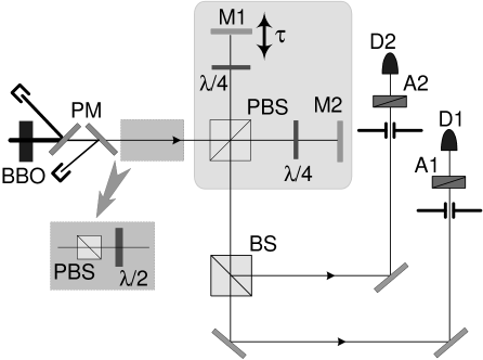
Figure 1: Experiment using collinear type-II SPDC. $\lambda/2$ plate is oriented at $22.5^{\circ}$ and $\lambda/4$ plates are oriented at $45^{\circ}$. Polarizer (PBS) and $\lambda/2$ plate set, shown in the inset, is inserted only when first-order interference is measured. Shaded area containing PBS, $\lambda/4$ plates, and mirrors is equivalent to commonly used quartz polarization delay.

Further evaluating Eq. (11) for $\theta_{1}=\theta_{2}=45^{\circ}$, we get

$$R_{c} = \int dt_{+}dt_{-}\int d\nu d\nu^{\prime}S(\nu)S(\nu^{\prime})e^{i(\nu-\nu^{\prime})\tau}$$

$$\times\sin(\nu t_{-})\sin(\nu^{\prime}t_{-}),$$

$$\approx \int d\nu|S(\nu)|^{2}-\int d\nu|S(\nu)|^{2}e^{-i2\nu\tau},$$

$$= 1-g^{(1)}(2\tau),$$

where $t_{-}=t_{2}-t_{1}$, $t_{+}=t_{1}+t_{2}$. In approximating the above equation, we’ve used the fact that $S(\nu)$ is an even function and $\nu$ is in optical frequency. The above equation can be re-written as

$$R_{c}=\frac{1}{2}\left\{1\pm g^{(1)}(2\tau)\right\},$$ (12)

where $-$ sign is for $\theta_{1}=\theta_{2}=45^{\circ}$ and $+$ sign is for $\theta_{1}=-\theta_{2}=45^{\circ}$.

It is interesting to note that the two-photon wavepacket, eq. (12), does not contain the second-order correlation function $G^{(2)}(\tau)$. This result has interesting implications: (i) $R_{c}$ has the same envelope as $R_{s}$ except that the $R_{c}$ envelope is half of the $R_{s}$ envelope, (ii) any dispersion element introduced in a Shih-Alley/Hong-Ou-Mandel interferometer cannot affect the shape of the interference envelope since $g^{(1)}(\tau)$ is not affected by group velocity dispersion note2 .

IV Experiment

In this section, we describe two experiments which are designed to test the predictions made in section III. For both type-I and type-II SPDC experiments, the pump laser was a argon ion laser operating at 351.1 nm. Coincidence counts were measured using a time-to-amplitude converter (TAC) and multi-channel analyzer (MCA) set. The coincidence window used for second-order interference measurement was 3 nsec.

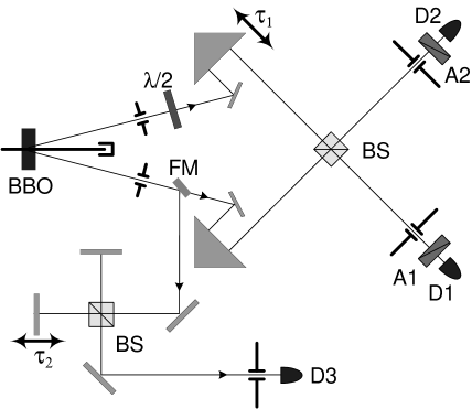
Figure 2: Experimental setup using non-collinear type-I SPDC. $\lambda/2$ plate rotates the polarization of the signal photon from horizontal to vertical. FM is a flipper mirror.

Let us first describe the wavepacket measurement of type-II SPDC. The experimental setup can be seen in Fig. 1. A 2 mm thick type-II BBO crystal was pumped by a 351.1 nm laser beam generating 702.2 nm collinear type-II SPDC photons. The residual pump beam was removed by two pump reflecting mirrors (PM). Instead of using usual quartz delay line for introducing fine delay between horizontal and vertically polarized photons shih2 ; shih3 , a set of PBS, $\lambda/4$ plates (oriented at $45^{\circ}$), and mirrors (shown in the shaded area) was used. The inset containing a PBS and a $\lambda/2$ plate (oriented at $22.5^{\circ}$) was used to remove vertically polarized photons when measuring first-order interference. The delay between the two arms of the interferometer was introduced by moving mirror M1 with an encoder driver. Photons were finally detected with detector packages which consist of a single-photon counting module and a polarization analyzer. The distance from the BBO crystal to the detector was approximately 218 cm and all apertures used in this experiment were about 3 mm in diameter.

Fig. 3 shows the experimental data for the type-II SPDC experiment. Fig. 3(a) shows first-order interference of the horizontal polarized photon. As discussed above, vertical polarized photons are removed with a PBS and a $\lambda/2$ plate is used to rotate the polarization direction to $45^{\circ}$. For this measurement, we used a 20 nm FWHM filter to suppress the white-light interference which occurs around $\tau=0$ strekalov . The observed triangular one-photon wavepacket agrees well with the theoretical prediction shown in Fig. 4(a).

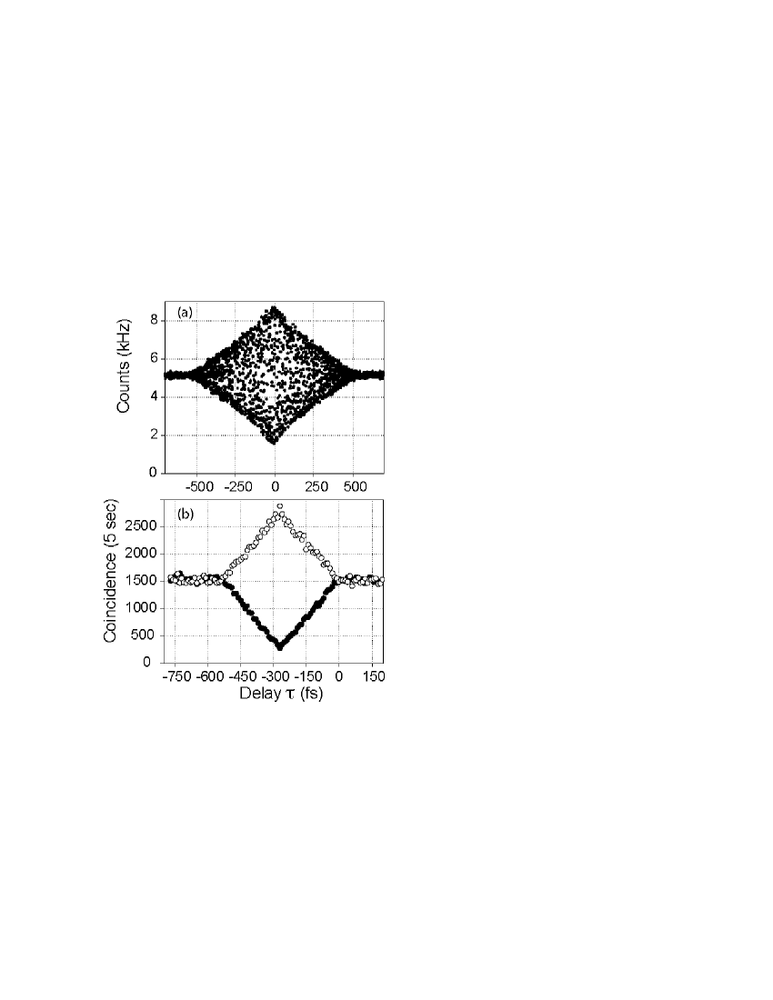
Figure 3: Experimental data for type-II SPDC. (a) First-order interference. (b) Second-order interference. Solid circles are for $\theta_{1}=\theta_{2}=45^{\circ}$ and empty circles are for $\theta_{1}=-\theta_{2}=45^{\circ}$, where $\theta_{1}$ and $\theta_{2}$ are analyzer (A1 and A2) angles. Peak-dip visibility is about 84 %. Coincidence peak or dip occurs when the e-polarized photons are delayed by $D\times L/2\approx 247$ fs with respect to the o-polarized photons before reaching the beamsplitter BS.

To measure the two-photon wavepacket, we first removed the PBS-$\lambda/2$ plate set used for first-order interference measurement. The e-ray of the crystal (vertically polarized photons) could then be delayed with respect to the o-ray by moving M1. For this measurement, only uv-cut off filters (cut-off at 550 nm) were used to suppress any residual pump noise. Fig. 3(b) shows typical triangular two-photon wavepacket observed in coincidence counts in which the dip or peak occurs when the e-polarized photons are delayed by $D\times L/2\approx 247$fs with respect to the o-polarized photons before reaching the beamsplitter BS shih2 ; shih3 . Again, the observed triangular two-photon wavepacket agrees well with the theoretical prediction shown in Fig. 4(b).

As we have predicted in the previous section, the one-photon and the two-photon wavepackets have the same shapes and the one-photon wavepacket is twice bigger than the two-photon wavepacet. Although we here have used collinear type-II SPDC for one-photon and two-photon wavepacket calculation and measurements, recent experimental results confirm that non-collinear type-II SPDC gives the same result for the two-photon wavepacket measurement kg1 ; kg . Finally, we note that the power spectrum function, in type-II SPDC, includes parameters of both the signal and the idler photons (in $D=dK_{i}/d\Omega_{i}-dK_{s}/d\Omega_{s}$) even though only one of them is actually measured strekalov .

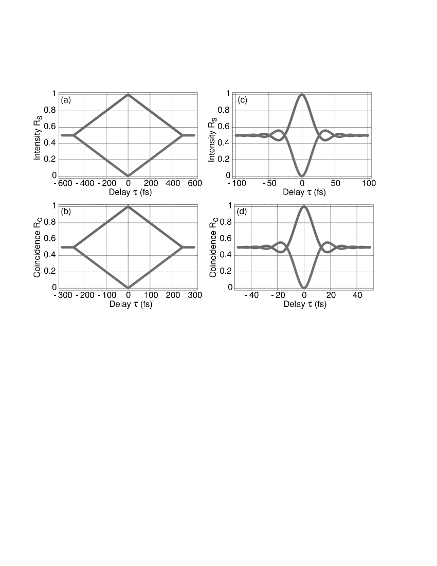
Figure 4: Calculated first- and second-order interference patterns for type-II SPDC, (a) and (b), and type-I SPDC, (c) and (d). Only the fringe envelopes are shown for the first-order interference $R_{s}$. It is clear that $R_{s}$ and $R_{c}$ have the same envelope shapes. However, the width of the coincidence envelope is half of that of first-order interference ($R_{s}$). The plots are calculated for the following parameters: BBO crystal with 2 mm thickness, 351.1 nm pump wavelength, and 702.2 nm SPDC central wavelength. For (b), the delay is shifted by $D\times L/2\approx 247$ fs for easy comparison with (a).

Let us now discuss the measurement of one-photon and two-photon wavepackets for type-I SPDC. The experimental setup can be seen in Fig. 2. The pump laser beam was centered at 351.1 nm and 702.2 nm centered SPDC photons were generated from a 2 mm thick type-I BBO crystal. The propagation angle of the signal-idler photon pair was about $\pm 3^{\circ}$ with respect to the pump beam propagation direction. A $\lambda/2$ plate was used to rotate the signal photon’s polarization from horizontal polarization to vertical polarization. The signal-idler photons were then made to interfere at a beamsplitter and the delay $\tau_{1}$ was varied by an encoder driver driven trombone prism. Detectors D1 and D2 placed at the output ports of the beamsplitter were used for second-order interference measurement. For first-order interference measurement, a flipper mirror (FM) was used to direct the idler photon to the secondary Michelson interferometer. Interference was measured by detector D3 as a function of the arm length difference $\tau_{2}$. The crystal to the D3 distance was about 200 cm and to D2-D1 was about 280 cm. As before, all apertures used in this experiment were about 3 mm in diameter.

For one-photon wavepacket measurement, we used the flipper mirror (FM) to direct the idler photon to the secondary Michelson interferometer as shown in Fig. 2. First-order interference was observed by moving one of the mirror by an encoder driver and to reduce any residual pump noise, a uv-cutoff filter was used in front of the detector. The experimental data for this measurement can be seen in Fig. 5(a) and the envelope of first-order interference or one-photon wavepacket closely follows the predicted curve shown in Fig. 4(c). This confirms that the power spectrum of either the signal or the idler photon of type-I SPDC is indeed given by $|S(\omega-\Omega)|^{2}$.

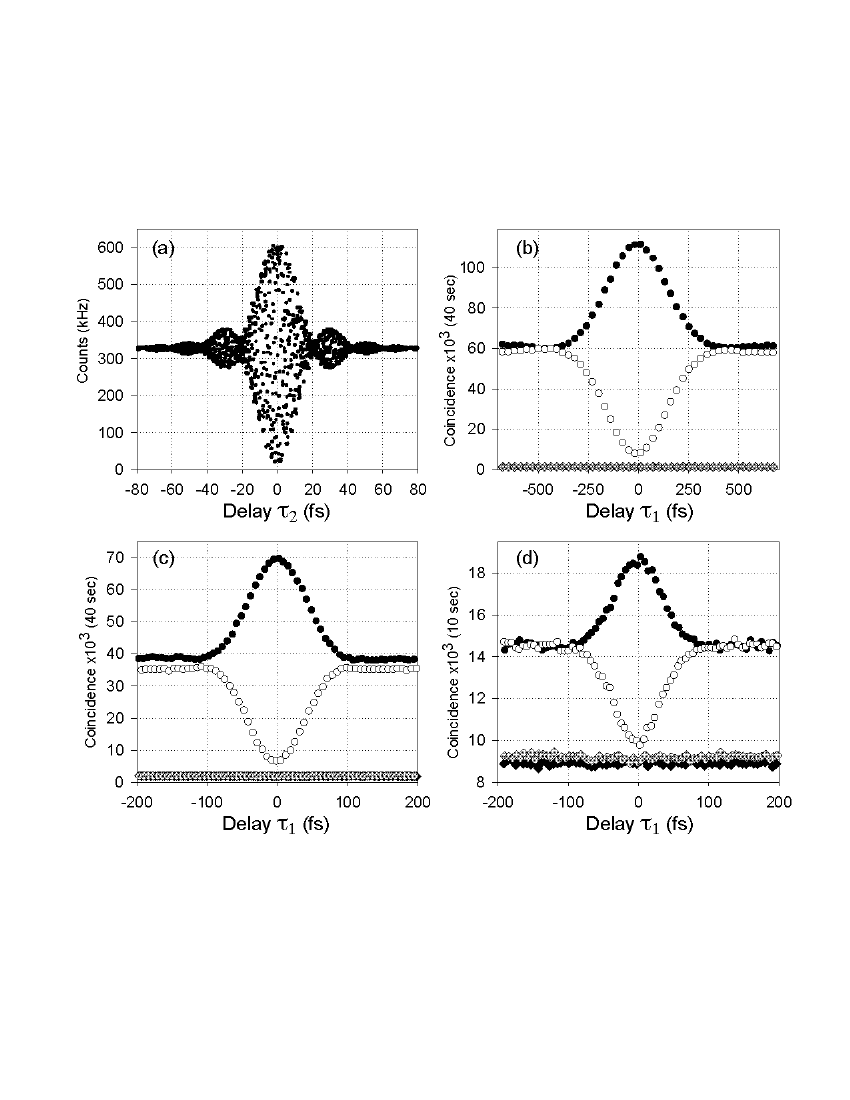
Figure 5: Experimental data for type-I SPDC experiment. (a) First-order interference. Only UV-cutoff filter (cutoff at 550 nm) is used to suppress the pump noise. The visibility is about 92%. (b), (c), and (d) show second-order interference measurements. Diamond data points show the level of accidental coincidence. Solid data points are for $\theta_{1}=-\theta_{2}=45^{\circ}$ and empty circles are for $\theta_{1}=\theta_{2}=45^{\circ}$. Spectral filters used for (b), (c), and (d), are 3 nm FWHM, 20 nm FWHM, and 80 nm FWHM, respectively.

For two-photon wavepacket measurement, we removed the flipper mirror (FM) and let the signal-idler photons interfere at the beamsplitter. The coincidence counts were measured as a function of both the delay $\tau_{1}$ and the analyzer angles. We also measured the true coincidence counts as well as accidental coincidence counts by integrating additional 3 nsec window which was located about 10 nsec away from the true coincidence peak in the MCA spectrum.

We first measured the two-photon wavepacket with 3 nm FWHM spectral filters. The data for this experiment can be seen in Fig. 5(b). The visibility for this measurement is quite high ($\sim 87$%), however, the two-photon wavepacket has quite different shape than the one-photon wavepacket, mostly due to narrow-band filtering of the SPDC photons by the 3 nm filters. We can roughly estimate the contribution of the spectral filters to the broadened coherence time by using $\tau_{c}\sim\lambda^{2}/(c\Delta\lambda)\approx 550$ fsec. Considering that the filters do not necessarily have perfect Gaussian shape transmission curve and they may have different FWHM values than the specified values, this rough estimation gives a pretty good idea on the origin of the broadened two-photon wavepacket. Note also that the level of accidental coincidence is nearly negligible.

The same measurement was repeated with two more sets of spectral filters: 20 nm FWHM and 80 nm FWHM. With 20 nm filters, see Fig. 5(c), we still observe quite good visibility of 83%. Notice that the level of accidental contribution has risen slightly and the two-photon wavepacket is now narrower. By using the simple picture again, we estimate $\tau_{c}\sim\lambda^{2}/(c\Delta\lambda)\approx 82$ fsec. This value is quite close to the observed two-photon wavepacket shown in Fig. 5(c) and it means that we are still observing a spectrally filtered, by the spectral filters, two-photon wavepacket.

Finally, 80 nm FWHM filters were used for the same measurement, see Fig. 5(d). We find that the raw visibility has now dropped to 32% with almost no change in the two-photon wavepacket. According to Fig. 4(d), the unfiltered two-photon wavepacket should be about 15 fsec in FWHM. Note also that the contribution of accidental coincidence is now significant, unlike Fig. 5(b) and Fig. 5(c).

This rather unexpected behavior of the two-photon wavepacket with broadband spectral filters can be understood as follows. It is well-known that type-I SPDC in general has much bigger bandwidth than type-II SPDC. Especially, for the case considered in this paper, the calculated FWHM of the type-I SPDC spectrum is more than 80 nm which is much bigger than roughly 3 nm calculated FWHM bandwidth of type-II SPDC. This calculation actually agrees quite well with the observed first-order interference shown in Fig. 3(a) and Fig. 5(a). Based on this observation alone, it may seem, at first, that the bandwidth of type-I SPDC is not limited at all at the detectors. To see what really is happening, however, it is necessary to consider the type-I SPDC tuning curve, which shows how SPDC spectrum is distributed as functions of propagation angles and wavelengths.

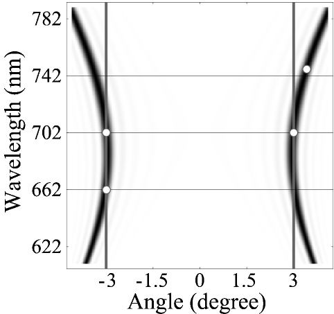
Figure 6: Tuning curve for non-collinear type-I SPDC used in this experiment. Two vertical bars located at $\pm 3^{\circ}$ represent the angles defined by the apertures. Left (right) curve shows the angle-spectrum distribution of the signal (idler) photons. See text for details.

Fig. 6 shows the tuning curve of non-collinear type-I SPDC used in this experiment. The left curve shows the angle-spectrum distribution for the signal photons and the right curve shows the same for the idler photons. Note that the signal and the idler photons have the same angle-spectrum distribution as both signal and idler photons have the same polarization. Two vertical bars represent the angles defined by the apertures used in the experiment.

For one-photon wavepacket measurement, only the signal or the idler photons are measured. If is clear from Fig. 6 that the signal or the idler photons indeed have quite broad bandwidth (more than 80 nm) even if we only consider the small angle defined by the aperture. It is because the slope of the tuning curve for type-I SPDC is not steep, unlike type-II SPDC. For second-order interference measurement, however, we need to consider signal-idler photon pair detections and the fact that their frequencies are anti-correlated, i.e., $\omega_{s}=\Omega+\nu$ and $\omega_{i}=\Omega-\nu$. If spectral filers have narrow bandwidths around 702.2 nm (shown as two circles at 702 nm in Fig. 6), we just need to consider the cross-sections of the vertical bars and small area around 702.2 nm. It is then easy to see that only frequency anti-correlated photon pairs can be detected almost all the time.

As we use spectral filters with broader bandwidths, the possibility of detecting uncorrelated photons gets bigger and bigger. It is because when the filter bandwidth is big, uncorrelated photons with large frequency difference can result in significant accidental coincidence counts because of the apertures used in the experiment. Let us consider an example: the signal photon is at 662 nm and, due to the energy conservation condition, the idler photon is at 748 nm (shown as two circles at 662 nm and 748 nm). The 662 nm signal photon can be detected. However, as we can see in Fig. 6, the 748 nm idler photon simply cannot be detected because it lies outside the detectable area in the tuning curve. Therefore, when broadband filters are used, the two-photon wavepacket is mainly determined by spatial filtering by apertures rather than spectral filters. Also, increased non-pair detection or uncorrelated photon detection due the use of broadband filters greatly increases the level of accidental coincidence counts, which in turn reduces the raw quantum interference visibility.

This effect is clearly demonstrated in Fig. 5(b) $\sim$ Fig. 5(d). Up to 20 nm filters, uncorrelated detection evens are still quite negligible as accidental coincidence counts do not reduce visibility much. With 80 nm filters, which accepts nearly full bandwidths of type-I SPDC, the accidental coincidence contribution is huge and this reduces the raw visibility significantly. Since such accidental coincidence counts from uncorrelated events produce a flat background, they can be subtracted from the overall coincidence counts (the corrected visibility increases to 86%).

It may be possible to remove such spectral filtering effect by removing the apertures altogether or opening them completely. However, this makes it nearly impossible to align and use the interferometer because spatial modes cannot be well defined and the accidental coincidence will increase significantly, just as in this experiment. We have indeed observed slight narrowing of two-photon wavepacket by opening the apertures, but, due to limited collection angles of our detection system, it was not possible to observe very short two-photon wavepacket predicted in section III. If the bandwidth of type-I SPDC is inherently narrow and the angle-wavelength tuning curve slope is steep, for example, by using a different non-linear crystal or using different phase matching scheme, such an effect may nevertheless be observed. For example, Burlakov et. al. in Ref. burlakov, observed a similar effect using collinear type-I SPDC from LiO₃ crystals, but the interferometric two-photon wavepacket measurement scheme involved two nonlinear crystals instead of one: i.e., the two-photon wavepacket was measured by interfering two-photon amplitudes from different crystals.

V Conclusion

We have measured one-photon and two-photon wavepackets of type-I and type-II SPDC generated from a cw laser pumped BBO crystal. In the case of type-II SPDC, the measured wavepackets agreed well with the theory. Although we used collinear type-II SPDC for these measurements, it was observed elsewhere that non-collinear type-II SPDC gives the same result kg1 ; kg .

In experiments involving type-I SPDC, even though the one-photon wavepacket measurement agreed well with the theory, the two-photon wavepacket was much bigger than the expected value. Upon studying the tuning curve of type-I SPDC from a BBO crystal, we found that spatial filtering limits the two-photon pair detection bandwidth even though one-photon bandwidth is not limited. Such spatial filtering is specific to the tuning curve characteristics of the nonlinear crystal and the geometry of the experiment. It may be avoided with the use of a nonlinear crystal which has sharp (non-collinear) angle-wavelength tuning characteristics or with the use of the collinear multi-crystal geometry burlakov .

In this paper, we have used well-known one-dimensional approximation when calculating one-photon and two-photon wavepackets. This approximation works well with both collinear and non-collinear type-II SPDC experiments with a BBO crystal. However, for broadband non-collinear type-I SPDC, it became clear that tuning curve characteristics of the crystal needs to be considered seriously.

Our results imply that one should be careful using non-collinear type-I SPDC in applications in which variables other than polarizations, such as energy and momentum, are important. One example of such possible applications is quantum metrology; care must be taken not to over-estimate the two-photon bandwidth. Our results also imply that generating high-purity polarization-entangled states or Bell-states using type-I non-collinear SPDC from a BBO crystal almost always rely on strong spectral post-selection, as increased detection bandwidths reduce the raw visibility significantly, even with a cw pump.

ACKNOWLEDGEMENTS

The author wishes to thank M.V. Chekhova for many enlightening discussions and W.P. Grice for helpful comments. This research was supported in part by the U.S. DOE, Office of Basic Energy Sciences, the National Security Agency, and the LDRD program of the Oak Ridge National Laboratory, managed for the U.S. DOE by UT-Battelle, LLC, under contract No. DE-AC05-00OR22725.

References

- (1) D.N. Klyshko, Photons and Nonlinear Optics (Gordon and Breach, New York, 1988).
- (2) C.K. Hong and L. Mandel, “Theory of frequency down conversion of light,” Phys. Rev. A 31, 2409-2418 (1985).
- (3) M.H. Rubin, D.N. Klyshko, Y.H. Shih, and A.V. Sergienko, “Theory of two-photon entanglement in type-II optical parametric down-conversion,” Phys. Rev. A 50, 5122-5133 (1994).
- (4) Y.H. Shih and C.O. Alley, in Proceedings of the Second International Symposium on Foundations of Quantum Mechanics in the Light of New Technology, Tokyo, 1986, edited by M. Namiki (Physical Society of Japan, Tokyo, 1987).
- (5) Y.H. Shih and C.O. Alley, “New Type of Einstein-Podolsky-Rosen-Bohm Experiment Using Pairs of Light Quanta Produced by Optical Parametric Down Conversion,” Phys. Rev. Lett. 61, 2921-2924 (1988).
- (6) C. K. Hong, Z. Y. Ou, and L. Mandel, “Measurement of subpicosecond time intervals between two photons by interference,” Phys. Rev. Lett. 59, 2044-2046 (1987).
- (7) Z. Y. Ou and L. Mandel, “Violation of Bell’s Inequality and Classical Probability in a Two-Photon Correlation Experiment,” Phys. Rev. Lett. 61, 50-53 (1988).
- (8) A.V. Burlakov, M.V. Chekhova, O.A. Karabutova, and S.P. Kulik, “Collinear two-photon state with spectral properties of type-I and polarization properties of type-II spontaneous parametric down-conversion: Preparation and testing,” Phys. Rev. A 64, 041803(R) (2001).
- (9) A. Valencia, M.V. Chekhova, A. Trifonov, and Y. Shih, “Entangled Two-Photon Wave Packet in a Dispersive Medium,” Phys. Rev. Lett. 88, 183601 (2002).
- (10) D.V. Strekalov, Y.-H. Kim, and Y. Shih, “Experimental study of a subsystem in an entangled two-photon state,” Phys. Rev. A 60, 2685-2688 (1999).
- (11) L. Mandel and E. Wolf, Optical coherence and quantum optics (Cambridge university press, New York, 1995).
- (12) It is possible to completely remove the group velocity dispersion effect from if the positive dispersion introduced in is matched with a negative dispersion introduced in , see Ref. franson, .
- (13) J.D. Franson, “Nonlocal cancellation of dispersion,” Phys. Rev. A 45, 3126-3132 (1992).
- (14) P.G. Kwiat, A.M. Steinberg, and R.Y. Chiao, “Observation of a “quantum eraser”: A revival of coherence in a two-photon interference experiment,” Phys. Rev. A 45, 7729-7739 (1992).
- (15) Y.H. Shih and A.V. Sergienko, “Two-photon anti-correlation in a Hanbury Brown-Twiss type experiment,” Phys. Lett. A 186, 29-34 (1994).
- (16) Y.H. Shih and A.V. Sergienko, “A two-photon interference experiment using type II optical parametric down conversion,” Phys. Lett. A 191, 201-207 (1994).
- (17) Dispersion cancellation experiment based on this effect is reported in Ref. steinberg, and Ref. steinberg2, . This is, however, different from Franson’s non-local cancellation of dispersion in described in Ref. franson, .
- (18) A.M. Steinberg, P.G. Kwiat, and R.Y. Chiao, “Dispersion cancellation and high-resolution time measurements in a fourth-order optical interferometer,” Phys. Rev. A 45, 6659-6665 (1992)
- (19) A.M. Steinberg, P.G. Kwiat, and R.Y. Chiao, “Dispersion cancellation in a measurement of the single-photon propagation velocity in glass,” Phys. Rev. Lett. 68, 2421-2424 (1992).
- (20) Y.-H. Kim and W.P. Grice, “Generation of pulsed polarization-entangled two-photon state via temporal and spectral engineering,” J. Mod. Opt. 49, 2309-2323 (2002).
- (21) Y.-H. Kim, S.P. Kulik, M.V. Chekhova, W.P. Grice, and Y. Shih, “Experimental entanglement concentration and universal Bell-state synthesizer,” Phys. Rev. A 67, 010301(R) (2003).