Numerical simulations of a quantum algorithm for Hilbert’s tenth problem

Abstract

We employ quantum mechanical principles in the computability exploration of the class of classically noncomputable Hilbert’s tenth problem which is equivalent to the Turing halting problem in Computer Science. The Quantum Adiabatic Theorem enables us to establish a connection between the solution for this class of problems and the asymptotic behaviour of solutions of a particular type of time-dependent Schrödinger equations. We then present some preliminary numerical simulation results for the quantum adiabatic processes corresponding to various Diophantine equations.

1 Hilbert’s tenth problem

One of the well-known and fascinating mathematical problems is about the existence of integer solutions of polynomial equations of the type

$$(x+1)^{3}+(y+1)^{3}-(z+1)^{3} \stackrel{{\scriptstyle?}}{{=}} 0.$$

According to Fermat’s last theorem, which has only been proved very recently, the above equation does not have any integer solution for $x$, $y$, and $z$. However, although it took hundreds of years for mathematicians to finally come up with such a proof, this proof may not be valid for similar equations such as

$$(x+1)^{3}+(y+1)^{3}-(z+1)^{3}+xyz \stackrel{{\scriptstyle?}}{{=}} 0.$$

Many important mathematical problems, such as Goldbach’s conjecture or the distribution of zeroes of Riemann Zeta function, can be cast into equivalent problems of whether related polynomial equations with integer coefficients have integer solutions or not. Because of this, David Hilbert in his famous list of mathematical problems in 1900 included as the tenth problem [1] the challenge:

Given any polynomial equation with any number of unknowns and with integer coefficients: To devise a universal process according to which it can be determined by a finite number of operations whether the equation has integer solutions.

Such equations are known as Diophantine equations. Never was it anticipated that this tenth problem is ultimately equivalent (as shown by Davis, Putnam, Robinson and Matiyasevich, see [1]) to the halting problem of Turing machines of more than 30 years later. On this equivalence basis it has been concluded that Hilbert’s tenth is not computable: there is no single universal process to determine the existence of integer solution or lack of it for arbitrarily given Diophantine equations in as far as there is no single universal machine to determine the halting or not of arbitrarily given Turing machine (which starts with some arbitrarily given input).

Thus, we would have to consider anew each different case of Diophantine equation.

In spite of this widely accepted result, we have proposed a quantum algorithm [2] for solving Hilbert’s tenth problem. In the next section we briefly summarise the algorithm. We then next present some preliminary numerical results from the simulations of quantum processes for some very simple Diophantine equations as a concrete “proof of concept”.

2 A quantum algorithm

2.1 General oracle for Hilbert’s tenth problem

It suffices to consider only nonnegative solutions of a Diophantine equation. Let us consider the example

$$(x+1)^{3}+(y+1)^{3}-(z+1)^{3}+cxyz=0, c\in Z,$$

with unknowns $x$, $y$, and $z$. Starting from the observation that if we can construct the hamiltonian

$$H_{P} = \left((a^{\dagger}_{x}a_{x}+1)^{3}+(a^{\dagger}_{y}a_{y}+1)^{3}-(a^{\dagger}_{z}a_{z}+1)^{3}+c(a^{\dagger}_{x}a_{x})(a^{\dagger}_{y}a_{y})(a^{\dagger}_{z}a_{z})\right)^{2},$$

which has a spectrum bounded from below in fact, and if we can obtain the corresponding ground state (of least energy) then we can solve the tenth problem!

The ground state $|g\rangle$ of the hamiltonian so constructed has the properties, for some $(n_{x},n_{y},n_{z})$,

$$N_{j}|g\rangle = n_{j}|g\rangle,$$

$$H_{P}|g\rangle = \left((n_{x}+1)^{3}+(n_{y}+1)^{3}-(n_{z}+1)^{3}+cn_{x}n_{y}n_{z}\right)^{2}|g\rangle\equiv E_{g}|g\rangle.$$

Thus a projective measurement of the energy $E_{g}$ of the ground state $|g\rangle$ will yield the answer for the decision problem: The corresponding Diophantine equation has at least one integer solution if and only if $E_{g}=0$, and has not otherwise. (If $c=0$ in our example, we know that $E_{g}>0$ from the Fermat’s last theorem.)

From the above observation, our ground-state oracle is thus clear:

1. Given a Diophantine equation with $K$ unknowns $x$’s

   $$D(x_{1},\cdots,x_{K}) = 0,$$ (1)

   we need to simulate on some appropriate Fock space the quantum hamiltonian

   $$H_{P} = \left(D(a^{\dagger}_{1}a_{1},\cdots,a^{\dagger}_{K}a_{K})\right)^{2}.$$ (2)

2. Measurement results of appropriate observables in the ground state will provide the answer for our decision problem.

One way, which is by no mean the only way, to obtain the ground state is guaranteed by the quantum adiabatic theorem [4] which we will exploit in the next section.

2.2 Quantum Adiabatic Algorithm

In the adiabatic approach [5], one starts with a hamiltonian $H_{I}$ whose ground state $|g_{I}\rangle$ is readily achievable. Then one forms a “slowly” varying hamiltonian which interpolates between $H_{I}$ and $H_{P}$ in the time interval $t\in[0,T]$

$${\cal H}(t/T) = \left(1-t/T\right)H_{I}+(t/T)H_{P},$$ (3)

$$\equiv H_{I}+(t/T)W.$$

We will adopt this approach with the proposed (universal) initial Hamiltonian

$$H_{I} = \sum_{i=1}^{K}(a^{\dagger}_{i}-\alpha^{*}_{i})(a_{i}-\alpha_{i})$$ (4)

which admits as the ground state the coherence state

$$|g_{I}\rangle=|\alpha_{1}\rangle\otimes\ldots|\alpha_{K}\rangle,$$ (5)

where $|\alpha_{i}\rangle=e^{-\frac{1}{2}|\alpha_{i}|^{2}}\sum_{n=0}^{\infty}\frac{\alpha_{i}^{n}}{\sqrt{n!}}|n\rangle.$

Provided the conditions of the adiabatic theorem [4] are observed, the initial ground state will evolve into our desirable ground state $|g\rangle$ up to a phase:

$$\lim_{T\to\infty}{\cal T}\exp\left\{-iT\int_{0}^{1}{\cal H}(\tau)d\tau\right\}|g_{I}\rangle = {\rm e}^{i\phi}|g\rangle,$$ (6)

where $\cal T$ is the time-ordering operator.

So our problem now is to solve the time-dependent Schrödinger equation for $t\in[0,T]$

$$i\partial_{t}\psi(t) = {\cal H}(t/T)\psi(t),\;t\in[0,T],$$ (7)

with the initial state being the coherence state (5).

We can analytically show in general the two crucial results below [3]:

• The ground state of ${\cal H}(t/T)$ is non-degenerate for $t\in(0,T)$. As the minimum energy gap between the ground state and the first excited state is non-zero, it takes only a finite time $T$ for the adiabatic process, as asserted by the quantum adiabatic theorem, to generate a state which has a high probability of being the ground state of $H_{P}$.

• The probability of the state at time $T$ in some number state, $|\langle\psi(T)|n_{0}\rangle|^{2}$, is greater than 1/2 iff $|n_{0}\rangle$ is the ground state of $H_{P}$. That is, we only need to solve the equation for increasing $T$ until this majority condition is satisfied in order to identify the ground state.

The proofs of these important results will be available elsewhere.

3 Simulation Technicalities

• We solve the Schrödinger equation numerically in some finitely truncated Fock space large enough to approximate the initial coherence state to an arbitrarily given accuracy. That is, a truncation $m$ is chosen such that

  $$|\alpha_{i};m\rangle=e^{-\frac{1}{2}|\alpha_{i}|^{2}}\sum_{n=0}^{m}\frac{\alpha_{i}^{n}}{\sqrt{n!}}|n\rangle$$ (8)

  has a norm less than one by some chosen $\epsilon$, $|1-\sqrt{\langle\alpha_{i};m|\alpha_{i};m\rangle}|\leq\epsilon$.

• At each time step $\delta t$, and up to $O(\delta t^{2})$,

  $$\psi(t+\delta t) = exp\{-i{\cal H}(t/T)\delta t\}\psi(t)=(1-i{\cal H}(t/T)\delta t-1/2{\cal H}^{2}(t/T)\delta t^{2})\psi(t),$$ (9)

  thus there are maximally only two creation operators, $a^{\dagger}_{i}a^{\dagger}_{j}$, and we can explore this fact to explore the infinite Fock space by increasing the size of the truncated Fock space by two at every time step.

• We employ the unitary solver, with conjugate gradient method,

  $$\psi(t+\delta t) = \frac{1-\frac{i}{2}{\cal H}(t/T)\delta t}{1+\frac{i}{2}{\cal H}(t/T)\delta t}\psi(t)$$ (10)

  which approximates $exp\{-i{\cal H}(t/T)\delta t\}$ to second order in $\delta t$. This solver, being unitary, preserves the norm of the state vector in the evolution of time even though the size of the underlying truncated Fock space is allowed to increase with time if necessary.

• The time step $\delta t$ at time $t$ is a function of time and is chosen in such a way that halving this $\delta t(t)$ only results in $O(\delta t^{2})$ correction.

4 Simulation parameters and results

4.1 Equation $xy+x+4y-11=0$

This is an equation resulted from the factoring of the number 15 into two prime factors. Because of the nature of the problem we can fix the truncated size of our Fock space to be $(m_{x},m_{y})=(9,9)$ in order to have the norm of the state vector less than unity by an amount $\epsilon=10^{-2}$ at all times. In this and in all other simulations below we choose $\alpha_{x}=\alpha_{y}=(2.0,0.0)$.

In Fig. 1 we plot the magnitude square of maximum component (in terms of the Fock states) of the state vector as a function of the total evolution time $T$ in some arbitrary unit. Closed to below $T\sim 1500$, the maximum probability components of $|\psi(T)\rangle$ are dominant by some states, denoted by (blue) star and (green) triangle symbols, none of which are the ground state. In fact, they are, respectively, the first degenerate excited states $|n_{x},n_{y}\rangle=|4,1\rangle$ and $|3,1\rangle$ of $H_{P}$.

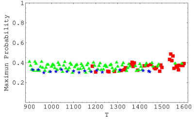
Figure 1: Corresponding equation $xy+x+4y-11=0$; with intermediate evolution time $T$.

With the increase in $T$ in Fig. 2, one of the Fock state, $|1,2\rangle$ denoted by (red) box symbol, has probability greater than $\frac{1}{2}$ which is our criterion for being identified as the ground state. We mark this regime as the quantum adiabatic regime when the ground state wins the battle for dominance.

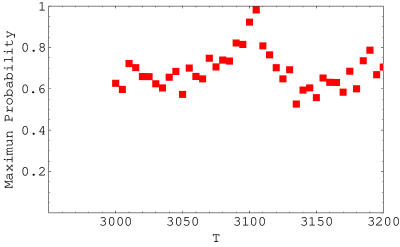
Figure 2: Corresponding equation $xy+x+4y-11=0$; with $T$ entering the quantum adiabatic regime.

From the ground state so identified we can infer that our Diophantine equation has one solution in this domain.

4.2 Equation $x+20=0$

We consider this extremely simple equation as an example which has no solution in the positive integers. The simulation parameters are as in the previous, except that the truncated size of our Fock space, starting with size 8, is now allowed to vary with time in order to simulate the exploration of the whole infinite space.

In Fig. 3 we plot the probabilities of the dominant components as a function of $T$. Below $T\sim 50$ none of the two components is greater than one-half, and in fact the first excited state, $|1\rangle$ denoted by (blue) triangle symbol, clearly dominates in this regime. Eventually we enter the quantum adiabatic regime upon when the (red) box symbol rises over the one-half mark; indeed it corresponds to the Fock state $|0\rangle$ which is the true ground state and which implies that our original Diophantine equation has no integer solution at all.

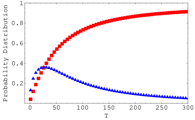
Figure 3: Corresponding equation $x+20=0$.

4.3 Equation $x-20=0$

We now consider a simple example which nevertheless has all the interesting ingredients typical for a general simulation of our quantum algorithm. Here we choose $\epsilon=10^{-3}$ and the initial Fock space has only up to $|n\rangle=|14\rangle$, which does not include the true ground state of $H_{P}$. This is typical in our simulations since we in general would not be able to tell in advance whether our initial Fock spaces do contain the true ground states or not. Generally, they do not. Even so, our strategy of allowing the expansion in the size of truncated Fock space in time has enabled the true ground state to be found and identified.

In this example, the state $|20\rangle$, which is not included in the initial truncated Fock space, is eventually reached and identified as the ground state as shown as red boxes in Fig. 4. Blue triangles and green stars are corresponding to the first two excited states $|19\rangle$ and $|21\rangle$, which are degenerate eigenstates of $H_{P}$.

Note that these competing pretenders somehow have unexpectedly probabilities greater than one-half (around $T\sim 90$), contrary to our analytical result that only the ground state can have probability rising above one-half! We think that this is only some artefact of finite-size time steps $\delta t$, and expect that it would go away once we employ a more sophisticated method for solving the Schrödinger equation. Work is in progress to systematically extrapolate to zero-size time steps to confirm the removal of this type of finite-size effects.

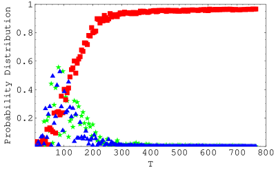
Figure 4: Corresponding equation $x-20=0$.

Figs. 5 and 6 depict the expectation values of occupation number and of energy as functions of $T$. They are, respectively, approaching 20 and zero (which signify the fact that our equation has an integer solution, namely 20).

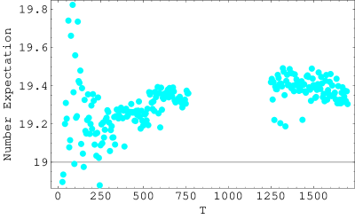
Figure 5: The expectation value of occupation number, $\langle N\rangle$, as a function of $T$.

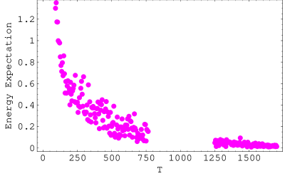
Figure 6: The expectation value of energy, $\langle H_{P}\rangle$, as a function of $T$.

5 Concluding Remarks

We here consider the issue of computability in principle, not that of computational complexity. The simulation results support the idea of implementation and execution of our quantum algorithm with a physical process [2]:

• Run the physical process (corresponding to the Diophantine equation in consideration) for some time $T$.

• Repeat the process at this $T$ to obtain the statistics through measurements.

• If none of the measurement outcomes exhibits probability of more than 1/2, ram up the $T$ and go back to the step above.

• Eventually, at some sufficiently large $T$, the measurement state with more-than-even probability can thus be identified as the ground state, terminating our physical implementation and execution.

• Substituting the quantum numbers for the now identified ground state enables us to see if $E_{g}=0$ and thus whether the Diophantine equation has a solution.

- [1] Y. Matiyasevich, Hilbert’s tenth problem, MIT Press, 1993.
- [2] Tien D. Kieu, “Computing the non-computable,” Contemporary Physics 44, 51-71, 2003; “Quantum algorithm for the Hilbert’s tenth problem,” E-print archive quant-ph/0110136v2 and references therein, 2001; “Gödel’s incompleteness, Chaitin’s number and Quantum Physics,” E-print archive quant-ph/0111062v2 and references therein, 2001; “A reformulation of the Hilbert’s tenth problem,” E-print archive quant-ph/0111063v1 and references therein, 2001.
- [3] Tien D. Kieu, in preparation.
- [4] A. Messiah, Quantum Mechanics, Wiley & Sons, 1958.
- [5] E. Farhi, J. Goldstone, S. Gutmann and M. Sipser, Quantum computation by adiabatic evolution, quant-ph/0001106, 2000.