Quantum walks on cycles

Abstract

We consider asymptotic behaviour of a Hadamard walk on a cycle. For a walk which starts with a state in which all the probability is concentrated on one node, we find the explicit formula for the limiting distribution and discuss its asymptotic behaviour when the length of the cycle tends to infinity. We also demonstrate that for a carefully chosen initial state, the limiting distribution of a quantum walk on cycle can lie further away from the uniform distribution than its initial state.

I Introduction

Celebrated results of Shor Shor (1994) and Grover Grover (1977) started a quest for algorithms based on quantum mechanics which can surpass corresponding classical algorithms. As many classical algorithms employ properties of random walks on graphs, several groups of researchers have begun to study properties of quantum analogues of classical random walks (for a survey see Kempe (a)). Two models of quantum random walks have been proposed by Aharonov et al. Aharonov et al. and Farhi and Gutmann Farhi ; in the paper we consider only a discrete quantum walk as defined in Aharonov et al. . The behavior of quantum random walks have been shown to differ greatly from their classical counterparts. Ambainis et al. Ambainis et al. proved that the spreading time in the quantum walk on line scales linearly with the number of steps, while Aharonov et al. Aharonov et al. showed that the mixing time for a walk on a cycle grows linearly with the cycle length. Even more spectacular exponential speed up was discovered by Kempe et al. Kempe (b) who studied a quantum random walk on hypercube; this result led to the construction of the first quantum algorithm based on a random walk by Shenvi et al. Shenvi et al. . The fact that in quantum walks on graphs the probability function spreads out much faster than in classical case is not the only factor which can be explored in designing new quantum algorithms. In Aharonov et al. the authors remarked that ‘one may try to use quantum walks which converge to limiting distribution which are different than those of the corresponding classical walks’. In this note we follow this suggestion and study the limiting distribution of a random walk on a cycle; it turns out that it depends on the length of the cycle in a somewhat surprising way. We also give an example of a quantum walk in which the distance from the initial state to the uniform distribution is larger than the distance between the uniform distribution and the initial state. Finally, we remark that recently Travaglione and Milburn Travaglione and Milburn (2002) and Dür et al. Dür et al. (2002) have proposed a scheme of experiment which realizes a quantum walk on a cycle.

II Model

We study a quantum random walk on a cycle with $d$ nodes. In the model of such a walk proposed in Aharonov et al. nodes are represented by vectors $|v\rangle$, $v=0,1,\dots,d-1$, which form an orthonormal basis of the Hilbert space $H_{V}$. An auxiliary two-dimensional Hilbert space $H_{A}$ (coin space) is spanned by vectors $|s\rangle$, $s=0,1$. The initial state of the walk is a normalized vector

$$|\Psi_{0}\rangle=\sum_{s,v}\alpha_{sv}|s,v\rangle=\sum_{s,v}\alpha_{sv}|s\rangle|v\rangle$$ (1)

from the tensor product $H=H_{A}\otimes H_{V}$. In a single step of the walk the state changes according to the equation

$$|\Psi_{n+1}\rangle=U|\Psi_{n}\rangle,$$ (2)

where the operation $U=S(H\otimes I)$ first applies the Hadamard gate operator $H=\sum_{s,s^{\prime}}(-1)^{ss^{\prime}}|s\rangle\langle s^{\prime}|$ to the vector from $H_{A}$, and then shifts the state by the operator

$$S=\sum_{s,v}|s\rangle\langle s|\otimes|v+2s-1({\rm mod}\ d)\rangle\langle v|\,.$$ (3)

The probability distribution on the nodes of the cycle after the first $n$ steps of the walk is given by

$$p_{n}(v)=\sum_{s}|\langle s,v|\Psi_{n}\rangle|^{2}.$$ (4)

However, as was observed by Aharonov at el. Aharonov et al. , for a fixed $v$, the probability $p_{n}(v)$ is ‘quasi-periodic’ as a function of $n$ and thus, typically, it does not converge to a limit. Thus, instead of $p_{n}(v)$ the authors of Aharonov et al. considered

$$\bar{p}_{n}(v)=\frac{1}{n}\sum_{i=1}^{n}p_{n}(v),$$ (5)

and proved that for any initial state $|\Psi_{0}\rangle$ and every node $v=0,1,\dots,d-1$, the sequence $\bar{p}_{n}(v)$ converges to the limiting distribution

$$\pi(v)=\sum_{a,a^{\prime}}\sum_{s}\Gamma_{aa^{\prime}}|\langle\phi_{a}|\Psi_{0}\rangle\langle\Psi_{0}|\phi_{a^{\prime}}\rangle\langle s,v|\phi_{a}\rangle\langle\phi_{a^{\prime}}|s,v\rangle,$$ (6)

where $c_{a}$ are the eigenvalues of $U$, $|\phi_{a}\rangle$ stand for the eigenvectors of $U$, and

$$\Gamma_{aa^{\prime}}=\begin{cases}1&\quad{\rm if}\quad c_{a}=c_{a^{\prime}}\\ 0&\quad{\rm if}\quad c_{a}\neq c_{a^{\prime}}.\end{cases}$$ (7)

In the case of the Hadamard walk on cycle, for $j=0,1$ and $k=0,1,\dots,d-1$, we get

$$c_{jk}=\frac{1}{\sqrt{2}}\big{(}(-1)^{k}\sqrt{1+\cos^{2}(2\pi j/d)}-i\sin(2\pi j/d)\big{)},$$ (8)

and

$$|\phi_{jk}\rangle=(a_{jk}|0\rangle+a_{jk}b_{jk}|1\rangle)\otimes\sum_{v}\omega_{d}^{jv}|v\rangle,$$ (9)

where $\omega_{d}=e^{2\pi i/d}$,

$$a_{jk} =1\Big{/}\sqrt{d(1+|b_{jk}|^{2})},$$ (10)

$$b_{jk} =\omega_{d}^{j}\big{(}(-1)^{k}\sqrt{1+\cos^{2}(2\pi j/d)}-\cos(2\pi j/d)\big{)}.$$ (11)

Note that $c_{j0}\neq c_{j^{\prime}1}$ so $\Gamma_{jk,j^{\prime}k^{\prime}}=\gamma_{jj^{\prime}}\delta_{kk^{\prime}}$, where $\delta_{kk^{\prime}}$ is the Kronecker delta. Thus, (6) becomes

$$\pi(v)=\sum_{j,j^{\prime}}\sum_{k}\gamma_{jj}|\langle\phi_{jk}|\Psi_{0}\rangle\langle\Psi_{0}|\phi_{j^{\prime}k}\rangle A_{jj^{\prime}k}\omega_{d}^{v(j-j^{\prime})},$$ (12)

where $A_{jj^{\prime}k}=a_{jk}a_{j^{\prime}k}(1+b_{jk}b^{*}_{j^{\prime}k})$. If $d$ is odd, then all eigenvalues are distinct, $\gamma_{jj^{\prime}}=\delta_{jj^{\prime}}$, and $A_{jjk}=1/d$; consequently, $\pi(v)=(1/d)\sum_{j}\sum_{k}|\langle\phi_{jk}|\Psi_{0}\rangle|^{2}=1/d$. It comes as no surprise, since as was proved in Aharonov et al. Aharonov et al. the limiting distribution $\pi$ is always uniform in a non-degenerate case. Thus we concentrate on more interesting case of even $d$. Then, because of symmetries $c_{d/2-j,k}=c_{j,k}$ and $c_{d/2+j,k}=c_{jk}^{*}=c_{d-j,k}$, the coefficient $\gamma_{jj^{\prime}}$ does not vanish when one of the following conditions hold:

1. $j=j^{\prime}$;

2. $j=0$, $j^{\prime}=d/2$;

3. $j=t$, $j^{\prime}=d/2-t$, for $t=1,2,\dots,t_{\rm max}$;

4. $j=d-t$, $j^{\prime}=d/2+t$, for $t=1,2,\dots,t_{\rm max}$;

where here and below $t_{\rm max}=\lfloor(d-2)/4\rfloor$.

III Result and discussion

We study in detail the limiting distribution $\pi$ for a quantum walk for which starts with a state in which with probability one a particle is at a node $v_{0}$; more specifically we set

$$|\Psi_{0}\rangle=\frac{1}{\sqrt{2}}\big{(}|0,v_{0}\rangle+i|1,v_{0}\rangle\big{)}.$$ (13)

Then $\langle\phi_{jk}|\Psi_{0}\rangle=g_{jk}\omega_{d}^{-v_{0}j}$, where $g_{jk}=a_{jk}(1+ib^{*}_{jk})\big{/}\sqrt{2}$, and

$$\pi(v)=\sum_{j,j^{\prime}}\sum_{k}\gamma_{jj^{\prime}}f(j,j^{\prime},k)\omega_{d}^{(v-v_{0})(j-j^{\prime})},$$ (14)

with $f(j,j^{\prime},k)=g_{jk}g^{*}_{j^{\prime}k}A_{jj^{\prime}k}$. Since $\gamma_{jj^{\prime}}=0$ except of the four cases (i)–(iv) described above, we get

$$\pi(v)=F+(-1)^{\Delta}2{\rm Re}(F_{0})+(-1)^{\Delta}{\rm Re}\Big{(}\sum_{i=1}^{t_{\rm max}}F_{t}\Big{)},$$ (15)

where by

$$\Delta=\Delta(v)=\min\{|v-v_{0}|,d-|v-v_{0}|\}$$ (16)

denotes the distance between nodes $v_{0}$ and $v$, and

$$F =\sum_{j,k}f(j,j,k),$$ (17)

$$F_{0} =\sum_{k}f(0,d/2,k),$$

$$F_{t} =\sum_{k}f(t,d/2-t,k)+f(d/2+t,d-t,k).$$

After some elementary but not very exciting calculations (17) reduces to

$$F =\frac{1}{d},$$ (18)

$$F_{0} =0,$$

$$F_{t} =\frac{2}{d^{2}}\frac{\sin^{2}(2\pi t/d)}{1+\cos^{2}(2\pi t/d)}.$$

We remark that $F_{t}=0$ whenever $t_{\rm max}=0$, i.e., for $d=2$ and $d=4$. Hence the limiting distribution for even cycles of sizes two and four are uniform, which has also been observed by Travaglione and Milburn Travaglione and Milburn (2002), who analyzed a quantum walk on cycle of length four step by step. However, for $d\geq 6$ we have

$$\pi(v)=(1+\Pi(v))/d,$$ (19)

with the ‘correction’ term $\Pi(v)=(-1)^{\Delta}4S/d$, where

$$S=\sum_{t=1}^{t_{\rm max}}\cos(4\pi t\Delta/d)\Big{(}\frac{2}{1+\cos^{2}(2\pi t/d)}-1\Big{)}.$$ (20)

Setting $z=3-2\sqrt{2}\sim 0.17157\dots$, one can write (20) as

$$S=\Big{(}\frac{8z}{1-z^{2}}-1\Big{)}\sum_{t=1}^{t_{\rm max}}\cos(4\pi\Delta t/d) +\frac{8z}{1-z^{2}}\sum_{m=1}^{\infty}(-z)^{m}\sum_{t=1}^{t_{\rm max}}\cos(4\pi(\Delta+m)t/d)$$ (21)

$$+\frac{8z}{1-z^{2}}\sum_{m=1}^{\infty}(-z)^{m}\sum_{t=1}^{t_{\rm max}}\cos(4\pi(\Delta-m)t/d),$$

which, in turn, transforms to

$$S=-\frac{d}{4}(\delta_{\Delta,0}+\delta_{\Delta,d/2})+ (-1)^{\Delta}\frac{d}{4}\,\frac{8z}{1-z^{2}}\,\frac{z^{-\Delta}(-z)^{d/2}+z^{\Delta}}{1-(-z)^{d/2}}$$ (22)

$$+\frac{1+(-1)^{\Delta}\xi}{2}-\frac{4z}{(1-z)^{2}}-\frac{4z(-1)^{\Delta}\xi}{(1+z)^{2}},$$

where $\xi=\big{(}1+(-1)^{d/2}\big{)}\big{/}2$, i.e., $\xi=1$ when $d/2$ is even, and $\xi=0$ if $d/2$ is odd. Thus, we arrive at

$$\Pi(v)=(-1)^{\Delta+1}(\delta_{\Delta,0}+\delta_{\Delta,d/2})+ \frac{8z}{1-z^{2}}\,\frac{z^{-\Delta}(-z)^{d/2}+z^{\Delta}}{1-(-z)^{d/2}}$$ (23)

$$+\frac{4}{d}\Big{(}\frac{\xi+(-1)^{\Delta}}{2}-\frac{4(-1)^{\Delta}z}{(1-z)^{2}}-\frac{4z\xi}{(1+z)^{2}}\Big{)}.$$

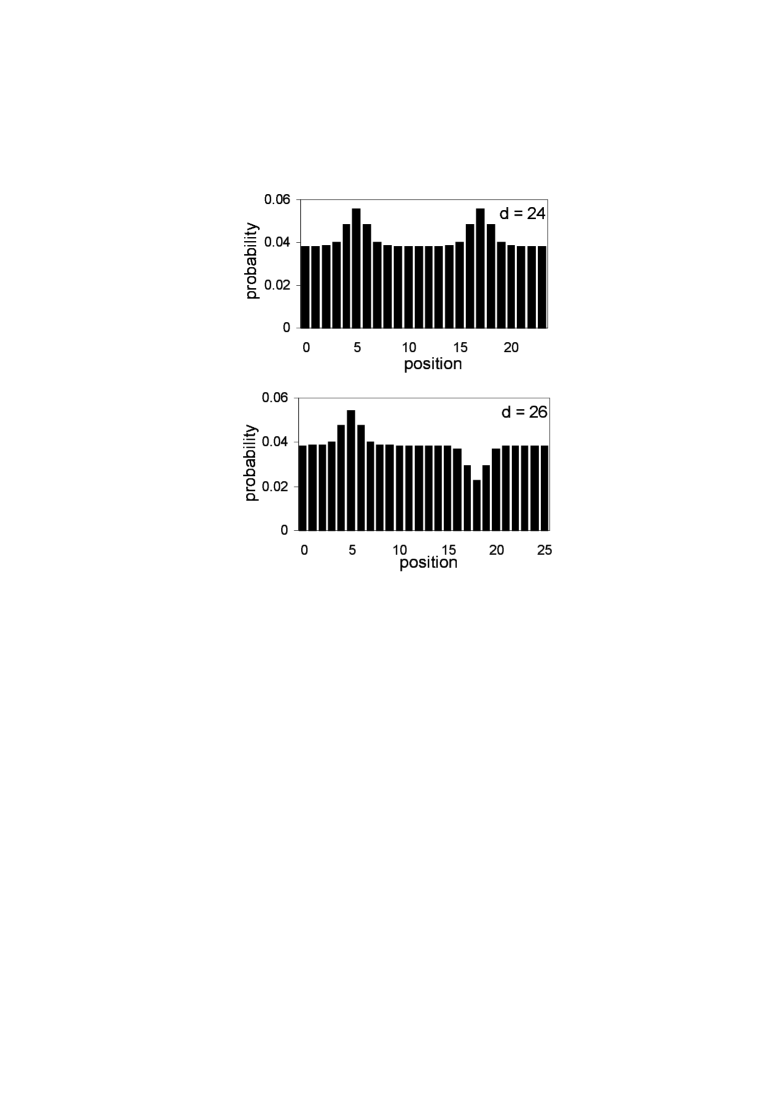
Figure 1: The limiting distributions for the cases of $d=24$ and $d=26$. The walk starts with the state where with probability one a particle is at the node $v_{0}=5$.

In Figure 1 we pictured the resulting limiting distributions for $d=24$ and $d=26$. It is easy to see they are almost uniform except for the nodes which lie next to the initially populated node $v_{0}$ and the opposite node $\hat{v}_{0}=v_{0}+d/2$ $({\rm mod}\ d)$. Indeed, as $d\to\infty$, the last term of (23) vanishes and

$$\bar{\Pi}(v)=\lim_{d\to\infty}\Pi(v)=\eta(\Delta)-(-1)^{\xi}\eta(\Delta^{\prime}),$$ (24)

where

$$\eta(x)=\frac{8z^{1+x}}{1-z^{2}}-\delta_{x0},$$ (25)

and $\Delta^{\prime}$ is the distance between nodes $v$ and $\hat{v}_{0}$. The equation (24) shows that the correction term $\bar{\Pi}(v)$ is significant only for $v$ which lie close to either $v_{0}$ or $\hat{v}_{0}$ and decreases exponentially with the distance between $v$ and $v_{0}$ and $\hat{v}_{0}$. Note that the shapes of the cusps near $v_{0}$ and $\hat{V}_{0}$ does not depend very much on $d$ for large $d$ (except of the scaling factor $1/d$). However, if $d/2$ is odd then the limiting distribution $\pi(v)$ has a minimum at $\hat{v}_{0}$, while if $d/2$ is even the distribution has a peak $\hat{v}_{0}$, virtually identical with that which appear at $v_{0}$ (see Figures 1 and 2). The fact that such a local behaviour of the limiting distribution $\pi$ depends so strongly on ‘global’ properties of space, as the parity of $d/2$, is somewhat surprising. We hope that this and/or analogous phenomena can be used in constructing efficient quantum algorithms.

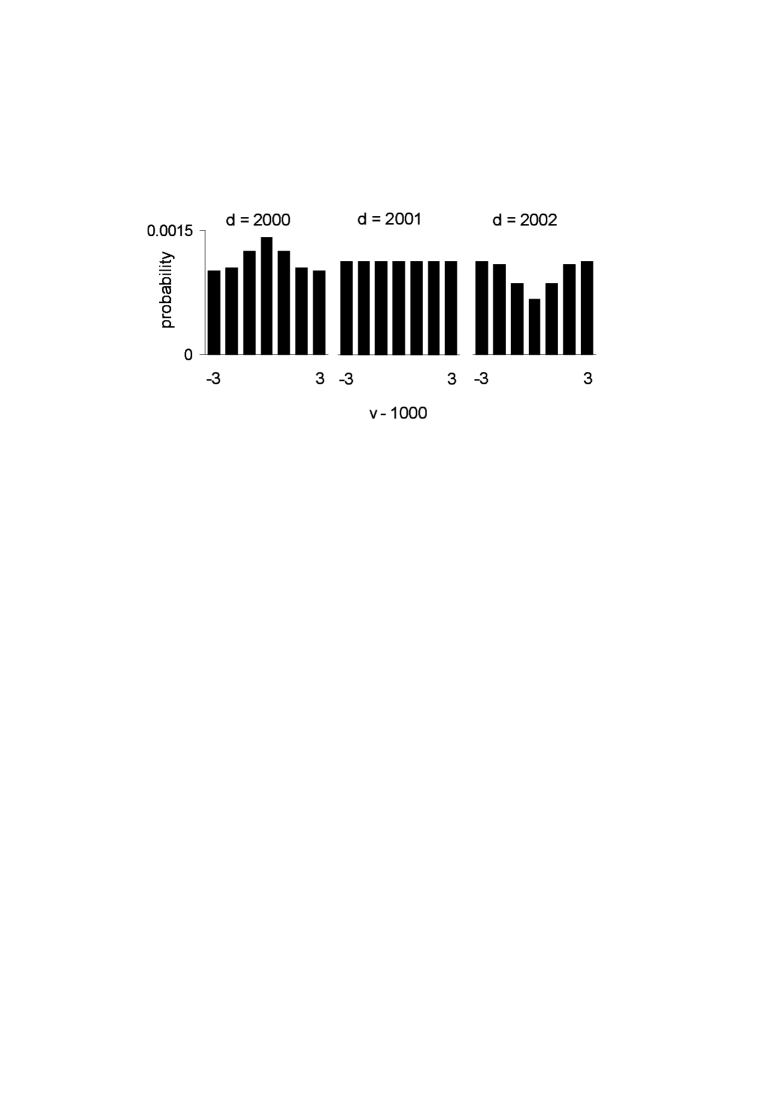
Figure 2: The limiting distribution for cycles of lengths $2000$, $2001$ and $2002$. In each case the walk starts with a state in which with probability one a particle is at $v_{0}=0$.

It is easy to see that, despite of a narrow cusps near nodes $v_{0}$ and $\hat{v}_{0}$, the total variation distance $d_{TV}$ between the limiting distribution given by (19) and (23) and the uniform distribution tends to 0 as $d\to\infty$. However it is not hard as well to construct ‘highly non-uniform’ distributions which remain invariant during the walk: one can simply take as the initial state a superposition of two degenerated eigenvectors (the distribution corresponding to a single eigenvector is always a uniform one). An example of such an invariant nonuniform probability distribution is presented on Figure 3.

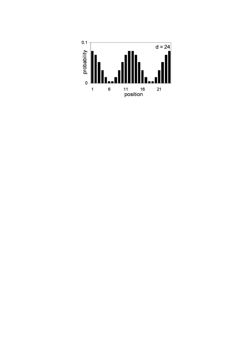
Figure 3: An example of a non-uniform invariant probability distribution for an initial state of the form $|\Psi_{0}=\frac{1}{\sqrt{2}}(|\phi_{5,0}\rangle+|\phi_{7,0}\rangle)$.

With a slightly more work one can construct the initial states which indicate differences between quantum and classical walks on cycles even more distinctively. One such example is shown on Figure 4. Here the total variation distance from the uniform distribution, defined as

$$\frac{1}{2}\sum_{v=0}^{d-1}\Big{|}p(v)-\frac{1}{d}\Big{|}$$ (26)

is equal $0.046$ for the initial state, while for the limiting distribution it grows to $0.204$.

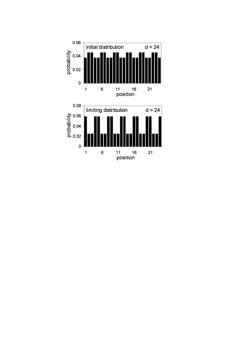
Figure 4: The initial and limiting distributions for the initial state $|\Psi_{0}\rangle=\frac{1}{2}(|\phi_{3,0}\rangle+|\phi_{9,0}\rangle-|\phi_{15,0}\rangle-|\phi_{21,0}\rangle)$.

IV Conclusion

We study the properties of a Hadamard quantum walk on a cycle with $d$ nodes. In the case of a walk starting from a single node we give an explicit formula for the limiting distribution and show that it is very sensitive to the arithmetic properties $d$. We hope that this or an analogous mode of behaviour can be used in construction of efficient quantum algorithms.

Furthermore, we present an example of a quantum walk on a cycle, for which the total variation distance between the initial distribution and the uniform distribution is much smaller than the distance between limiting distribution and the uniform one.