Automated Method for Building $CNOT$ Based Quantum Circuits for Boolean Functions

Abstract

In this paper we discuss an efficient technique that can implement any given Boolean function as a quantum circuit. The method converts a truth table of a Boolean function to the corresponding quantum circuit using a minimal number of auxiliary qubits. We give examples of some circuits synthesized with this technique. A direct result that follows from the technique is a new way to convert any classical digital circuit to its classical reversible form.

1 Introduction

Implementing Boolean functions on quantum computers is an essential aim, in the exploration of the benefits, which may be gained from systems operating by quantum rules. It is important to find the corresponding quantum circuits, which can carry out the operations we use to implement on our conventional computers. On classical computers, a circuit can be built for any Boolean function using AND, OR and NOT gates. This set of gates cannot, in general be used to build quantum circuits because the operations are not reversible [1]. A corresponding set of reversible gates must be used to build a quantum circuit for any Boolean operation. In classical computer science, many clever methods have been used to obtain more efficient digital circuits [2] for a given Boolean function. Recently, there have been efforts to find an automatic way to create efficient quantum circuits implementing Boolean functions. It is shown that [3] any unitary gate can be represented as a composition of simpler gates but it is not necessarily the most efficient circuit for this operation. A method proposed in [4] used a modified version of Karnaugh maps[2] and depends on a clever choice of certain minterm gates to be used in minimization process, however it appears that this method has poor scalability. Another work [5], includes a very useful set of transformations for quantum Boolean circuits and proposes a method for building quantum circuits for Boolean functions by using extra auxiliary qubits, however, this will increase the number of qubits to be used in the final circuits.

In our construction for building quantum circuits for Boolean functions, we will use only one auxiliary qubit; which we initially set to zero, to hold the result of the Boolean function, together with $CNOT$ based transformations (gates) which work as follows [5]: $CNOT\left({C|t}\right)$ is a gate where the target qubit $t$ is controlled by a set of qubits $C$ such that $t\notin C$, the state of the qubit $t$ will be flipped from $\left|0\right\rangle$ to $\left|1\right\rangle$ or from $\left|1\right\rangle$ to $\left|0\right\rangle$ if and only if the conditions stated by the $CNOT$ gate is evaluated to true. The condition that a certain qubit evaluates to true depends on whether the state of the qubit is $\left|0\right\rangle$ (cond-0; $\delta$=1) or $\left|1\right\rangle$ (cond-1; $\delta$=0) according to the condition being set, where $\delta$ is a Boolean parameter that will be used in the Boolean algebraic expressions to indicate the condition being set on the qubit; i.e. the new state of target qubit $t$ is the result of $XOR$-ing the old state of $t$ with the $AND$-ing of the states of the control qubits $C$ (under the condition being set on each control qubit). For example, consider the $CNOT$ gate shown in Fig.1, it can be represented as $CNOT\left({\left\{{x_{1},\overline{x_{2}},x_{3}}\right\}|x_{4}}\right)$, where $\circ$ and $\bullet$ mean that the condition on the qubit will evaluate to true if and only if the state of that qubit is $\left|0\right\rangle$ (cond-0) and $\left|1\right\rangle$ (cond-1) respectively, while $\oplus$ denotes the target qubit which will be flipped if and only if all the conditions set on the control qubits being evaluated to true. This means that the state of the qubit $x_{4}$ will be flipped if and only if $x_{1}=x_{3}=\left|1\right\rangle$ and $x_{2}=\left|0\right\rangle$. In general, the target qubit in a 4–qubit gate will be changed according to the operation $x_{4}\to x_{4}\oplus\left({x_{1}\oplus\delta_{1}}\right)\left({x_{2}\oplus\delta_{2}}\right)\left({x_{3}\oplus\delta_{3}}\right)$, now to represent the gate shown in Fig.1, we will set $\delta_{1}=\delta_{3}=0$ and $\delta_{2}=1$, so the operation for this gate on $x_{4}$ will be $x_{4}\to x_{4}\oplus x_{1}\overline{x_{2}}x_{3}$,

Figure 1: $CNOT$ gate.

Some special cases of the general $CNOT$ gate have their own names, $CNOT$ gate with one control qubit with cond-1 is called Controlled-$Not$ gate; Fig.2(a), $CNOT$ gate with two control qubits both with cond-1 is called Toffoli gate; Fig.2(b), and $CNOT$ gate with no control qubits at all is called $NOT$ gate; Fig.2(c), where $C$ will be an empty set (C = $\Phi)$, we will refer to this case as $CNOT\left(x_{i}\right)$ where $x_{i}$ is the qubit which will be unconditionally flipped.

Figure 2: Special cases of the general $CNOT$ gate.

2 Quantum Boolean Function

A Boolean function, $F$, is a function that takes $n$ Boolean variables as inputs and gives one Boolean variable as output,

$$F(x_{1},x_{2},\ldots,x_{n})\to\left\{{0,1}\right\},x_{i}\in\left\{{0,1}\right\}\quad$$ (1)

To represent a Boolean function of $n-1$ inputs, a quantum circuit with $n$ qubits will be used where the extra qubit will be initialised with value $0$, this will then carry the result of the Boolean function at the end of the computation. Any Boolean function can be represented by a truth table, In order to be reversible; the truth table must have $n$ inputs and $n$ outputs. For example: Consider the Boolean function $F(x_{1},x_{2},x_{3})=\overline{x_{1}}+x_{2}x_{3}$, classically it’s truth table is represented as shown in Table.1 and for quantum computing purposes, the representation will be as shown in Table.2.

$x_{1}$	$x_{2}$	$x_{3}$	F
0	0	0	1
0	0	1	1
0	1	0	1
0	1	1	1
1	0	0	0
1	0	1	0
1	1	0	0
1	1	1	1

Table 1: Classical representation of the truth table for $F(x_{1},x_{2},x_{3})=\overline{x_{1}}+x_{2}x_{3}$.

$x_{1}$	$x_{2}$	$x_{3}$	$F_{ini}$	$x_{1}$	$x_{2}$	$x_{3}$	$F_{fin}$
0	0	0	0	0	0	0	1
0	0	1	0	0	0	1	1
0	1	0	0	0	1	0	1
0	1	1	0	0	1	1	1
1	0	0	0	1	0	0	0
1	0	1	0	1	0	1	0
1	1	0	0	1	1	0	0
1	1	1	0	1	1	1	1

Table 2: Quantum computing version of the truth table for $F(x_{1},x_{2},x_{3})=\overline{x_{1}}+x_{2}x_{3}$.

From the second representation, we can see that the $F_{ini}$ will be flipped only if the result of the function $F$ is 1, $F(x_{1},x_{2},x_{3})=1$.

3 Automatic Construction of Quantum Boolean Circuits

Stage 1:

A quantum Boolean circuit $U$ of size $m$ over $n$ qubit quantum system with qubits $\left|{x_{1}}\right\rangle,\left|{x_{2}}\right\rangle,\ldots,\left|{x_{n}}\right\rangle$ can be represented as a sequence of $CNOT$ gates [5],

$$U=CNOT\left({C_{1}|t_{1}}\right)\ldots CNOT\left({C_{i}|t_{i}}\right)\ldots CNOT\left({C_{m}|t_{m}}\right),\quad$$ (2)

where $t_{i}\in\left\{{x_{1},\ldots,x_{n}}\right\};\,\,C_{i}\subset\left\{{x_{1},\ldots,x_{n}}\right\};\,t_{i}\notin C_{i}$.

Using the modified truth table, we will choose $CNOT\left({C_{i}|t_{i}}\right)$ according to the following steps:

1. Select the input configurations from the truth table where $F_{fin}$ is 1.

2. Add a single $CNOT$ gate for every selected configuration taking the $F_{ini}$ as the target qubit.

3. Set the condition on the control qubit for gates being added according to it’s value in the configuration from the truth table, i.e. the qubit with value 0 in the truth table will be set to cond-0 in the corresponding $CNOT$ gate and the qubit with value 1 will be set to cond-1 in the corresponding $CNOT$ gate.

4. For input configurations where $F_{fin}$ is 0, we will not add any gates (as if we are applying identities on them).

For example, according to the truth table shown in Table.2, we will select only the configurations with $F_{fin}=1$ as shown in Table.3 and construct the corresponding quantum circuit as shown in Fig.3.

	$x_{1}$	$x_{2}$	$x_{3}$	$F_{fin}$
$G_{1}$	0	0	0	1
$G_{2}$	0	0	1	1
$G_{3}$	0	1	0	1
$G_{4}$	0	1	1	1
$G_{5}$	1	1	1	1

Table 3: Input configurations where $F(x_{1},x_{2},x_{3})=\overline{x_{1}}+x_{2}x_{3}=1.$

Figure 3: Initial quantum circuit for $F(x_{1},x_{2},x_{3})=\overline{x_{1}}+x_{2}x_{3}$.

The maximum number of CNOT gates we can add in this stage will be up to 2^n-1 CNOT gate where $n$ is the number of qubits in the quantum system.

Stage 2:

In the following transformations we will trace the operations being applied on the target qubit only, since no control qubits will be changed during the operations of the circuit. These circuit transformations are an extension and generalization of some of the equivalence between reversible circuits shown in [6]. We will apply this transformations on every $CNOT$ gate in the circuit we have, which will expand the number of $CNOT$ gates in the circuit, after which we will apply the Rule of Minimization on the whole circuit to get the final circuit, which implements the Boolean finction.

Let $x_{i}$’s be the control qubit, $x_{n}$ be the target qubits and $\delta_{i}\in\left\{{0,1}\right\}$ where i=1,2,…,$n$-1, the general operation to be applied on the target qubit is given by

$$x_{n}\to x_{n}\oplus\left({x_{1}\oplus\delta_{1}}\right)\left({x_{2}\oplus\delta_{2}}\right)\ldots\left({x_{n-2}\oplus\delta_{n-2}}\right)\left({x_{n-1}\oplus\delta_{n-1}}\right)\quad$$ (3)

Multiplying all terms we get the following transformation:

$$\begin{array}[]{l}x_{n}\oplus\left({x_{1}\oplus\delta_{1}}\right)\left({x_{2}\oplus\delta_{2}}\right)\ldots\left({x_{n-2}\oplus\delta_{n-2}}\right)\left({x_{n-1}\oplus\delta_{n-1}}\right)\\ =x_{n}\oplus x_{1}x_{2}\ldots x_{n-1}\oplus x_{1}x_{2}\ldots x_{n-2}\delta_{n-1}\oplus\ldots\oplus\delta_{1}x_{2}\ldots x_{n-1}\oplus\ldots\oplus\delta_{1}\delta_{2}\ldots\delta_{n-1}\\ \end{array}\quad$$ (4)

Examples

Example 1: If one control qubit with cond-0. Let $\delta_{1}$ = 1 as shown in Fig.4. The following two circuits are equivalent:

$$\begin{array}[]{l}CNOT(x_{1}).CNOT(\{x_{1},x_{2},\ldots,x_{n-1}\}|x_{n}).CNOT(x_{1}){\rm}\\ ={\rm}CNOT(\{x_{1},x_{2},\ldots,x_{n-1}\}|x_{n}).{\rm}CNOT(\{x_{2},{\rm}x_{3},{\rm}\ldots,{\rm}x_{n-1}\}|x_{n}){\rm}\\ {\rm}\\ \end{array}$$ (5)

Figure 4: $n$ qubit gate with only $\delta_{1}$=1 and it’s equivalent circuit.

Proof:

From Eqn.4, putting $\delta_{1}$ = 1 and $\delta_{i}=0;\,i=2,\ldots,n-1$ to get Eqn.6. The L.H.S. of Eqn.6 will represent L.H.S. circuit in Fig.4, and the R.H.S of Eqn.6 will represent the R.H.S. circuit in Fig.4.

$$x_{n}\oplus\overline{x_{1}}\,x_{2}\ldots x_{n-1}=x_{n}\oplus x_{1}x_{2}\ldots x_{n-1}\oplus x_{2}\ldots x_{n-1}\quad$$ (6)

Figure 5: $n$–qubit gate with $\delta_{1}$=1 and $\delta_{2}$=1 and it’s equivalent circuit.

Example 2: If two control qubit with cond-0. Let $\delta_{1}$ = 1 and $\delta_{2}$ = 1 as shown in Fig.5. The following two circuits are equivalent:

$$\begin{array}[]{l}CNOT(x_{1}).CNOT(x_{2}).CNOT(\{x_{1},x_{2},\ldots,x_{n-1}\}|x_{n}).\\ CNOT(x_{2}).CNOT(x_{1})=CNOT(\{x_{1},x_{2},\ldots,x_{n-1}\}|x_{n}).\\ CNOT(\{x_{2},{\rm}x_{3},\ldots,x_{n-1}\}|x_{n}).CNOT(\{x_{1},x_{3},\ldots,x_{n-1}\}|x_{n}).\\ CNOT(\{x_{3},x_{4},\ldots,x_{n-1}\}|x_{n})\\ \end{array}$$ (7)

Proof:

From Eqn.4, putting $\delta_{1}$ = 1, $\delta_{2}$ = 1 and $\delta_{i}=0;i=3,\ldots,n-1$ to get Eqn.8. The L.H.S. of Eqn.8 will represent the L.H.S. circuit in Fig.5, and the R.H.S of Eqn.8 will represent the R.H.S. circuit in Fig.5.

$$x_{n}\oplus\overline{x_{1}}\,\,\overline{x_{2}}\ldots x_{n-1}=x_{n}\oplus x_{1}x_{2}\ldots x_{n-1}\oplus x_{2}x_{3}\ldots x_{n-1}\oplus x_{1}x_{3}\ldots x_{n-1}\oplus x_{3}x_{4}\ldots x_{n-1}\quad$$ (8)

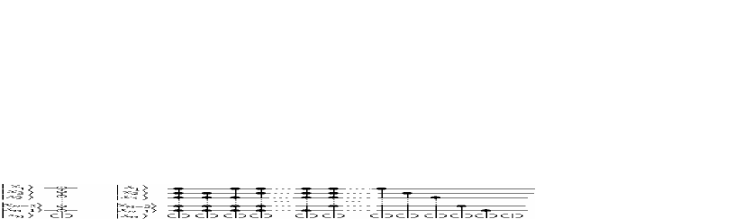
Figure 6: $n$–qubit gate with all $\delta_{i}$=1 and it’s equivalent circuit.

Example 3: The last possible case where all $\delta$’s will be equal to 1 as shown in Fig.6. The following two circuits are equivalent:

$$\begin{array}[]{l}CNOT(x_{1}).CNOT(x_{2})\ldots CNOT(x_{n-1}).CNOT(\{x_{1},x_{2},\ldots,x_{n-1}\}|x_{n}).\\ CNOT(x_{n-1})\ldots CNOT(x_{2}).CNOT(x_{1}){\rm}={\rm}CNOT(\{x_{1},x_{2},\ldots,x_{n-1}\}|x_{n}).\\ CNOT(\{x_{2},{\rm}x_{3},\ldots,{\rm}x_{n-1}\}|x_{n}).CNOT(\{x_{1},{\rm}x_{3},\ldots,{\rm}x_{n-1}\}|x_{n}).{\rm}\\ CNOT(\{x_{1},{\rm}x_{2},x_{4},\ldots,{\rm}x_{n-1}\}|x_{n})\ldots CNOT(\{x_{1},{\rm}x_{2},\ldots,{\rm}x_{n-3},{\rm}x_{n-1}\}|x_{n}).\\ CNOT(\{x_{1},{\rm}x_{2},\ldots,{\rm}x_{n-2}\}|x_{n})\ldots CNOT(\{x_{1}\}|x_{n}).{\rm}CNOT(\{x_{2}\}|x_{n})\\ \ldots CNOT(\{x_{n-1}\}|x_{n}).CNOT(x_{n})\\ \end{array}$$ (9)

Proof :

From Eqn.4; putting all $\delta_{i}$ = 1, $i$=1,…,$n$-1 to get Eqn.10, The L.H.S. of Eqn.10 represents the L.H.S. circuit in Fig.6 and The R.H.S. of Eqn.10 represents the R.H.S. circuit in Fig.6.

$$x_{n}\oplus\overline{x_{1}}\,\,\overline{x_{2}}\ldots\overline{x_{n-1}}=\overline{V},$$ (10)

where,

$$\begin{array}[]{l}V=x_{n}\oplus x_{1}x_{2}\ldots x_{n-1}\oplus x_{2}x_{3}\ldots x_{n-1}\oplus x_{1}x_{3}\ldots x_{n-1}\\ \oplus x_{1}x_{2}x_{4}\ldots x_{n-1}\oplus\ldots\oplus x_{1}x_{2}\ldots x_{n-3}x_{n-1}\oplus x_{1}x_{2}\ldots x_{n-2}\\ \oplus x_{1}\oplus x_{2}\oplus\ldots\oplus x_{n-1}\end{array}\quad$$

Applying these transformations on the circuit, we get from stage-1 we will get a new circuit with up to $3^{n-1}$ $CNOT$ gates.

Stage 3:

Now we have a quantum circuit where all $CNOT$ gates are applied on the target qubit $t$ with no control qubits with cond-0. In stage-3 of our method we carry out minimization to obtain the final simpler circuit. The method employs the following rule.

Rule of Minimization:

$$\begin{array}[]{l}CNOT(C_{i}|t).CNOT(C_{1}|t)\ldots CNOT(C_{n}|t).CNOT(C_{j}|t)\\ =CNOT(C_{1}|t)\ldots CNOT(C_{n}|t)\\ \end{array}\quad$$ (11)

if and only if $C_{i}=C_{j}$ as shown in Fig.7

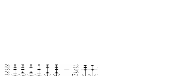
Figure 7: Rule of minimization.

Now applying this rule recursively on the circuit we have, we will get a new quantum circuit that on average (see next section) efficiently represents our Boolean function. For example, the final quantum circuit for $F(x_{1},x_{2},x_{3})=\overline{x_{1}}+x_{2}x_{3}$ is shown in Fig.8.

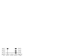
Figure 8: Final circuit for $F(x_{1},x_{2},x_{3})=\overline{x_{1}}+x_{2}x_{3}$.

4 Analysis and Results

Applying the above method on a truth table, after stage-1 the number of gates will be up to $2^{n-1}$ $CNOT$ gates with some controlled qubits with cond-0 and others with cond-1, the case where the number of $CNOT$ gates to be $2^{n-1}$ will occur only when all the $F_{fin}$ being set to 1 in the truth table, in this case the most optimum nonzero-gate circuit to be found using this method where only $CNOT(F_{ini})$ will exist in the final circuit as shown in Fig.9.

Figure 9: The most efficient non-zero gate with it’s truth table.

After stage-2, where the transformations being applied to eliminate all $\delta$’s equal to 1, we will be left with a new quantum circuit where the number of $CNOT$ gates will be up to $3^{n-1}$ gates. Starting the minimization of the circuit, analysing the method for $n$–qubit circuit, we get the following results: the number of possible circuits $S$ for all possible input configurations is given by

$$S=\sum\limits_{r=0}^{N}{\frac{N!}{r!(N-r)!}}=\sum\limits_{r=0}^{N}{{}^{N}C_{r}}\quad$$ (12)

where $N=2^{n-1}$ and $r$ is the number of $CNOT$ gates to be found in the final circuit.

From Eqn.12 we can see that the probability that the number of $CNOT$ gates in the final circuit is $2^{n-1}$ ($r=N$); which is the worst case, will be $1/S$ which means that the probability for this case will decrease as the number of qubits increase, similarly the probability that the final circuit to have zero-gates (identity; $r=0$) is $1/S$ which will decrease as the number of qubits increase as well. The most likely case to appear is the average where $r=2^{n-2}\left[{\pm 1}\right]$, for example consider a 3-qubit circuit: The number of possible circuits is 16 as shown in Fig.10 and the probability that a 4-gate circuit or 0-gate circuit to appear is 0.0625 and the probability that $2\left[{\pm 1}\right]$-gates circuit to appear is 0.875. And for a 4-qubit circuit: The number of possible circuits is 256 and the probability that an 8-gate circuit or 0-gate circuit to appear is 0.00390625 and the probability that $4\left[{\pm 1}\right]$-gates circuit to appear is 0.7109375.

There is no clear proof at this time that the cost of implementing multiple input $CNOT$ gates is higher than $CNOT$ gates with fewer inputs, but a further optimization for the cost of $CNOT$ gates used in this method can be achieved with a small increase in the number of $CNOT$ gates used by applying circuit reduction from the canonical form shown in [5].

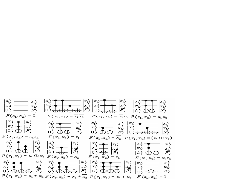
Figure 10: A complete set of a 3–qubit quantum circuits.

This method is also used to implement Boolean arithmetic operations like addition and multiplication and also used to implement $m$-to-$n$ Boolean logic, these results will be presented in a subsequent paper.

5 Comparing our Method with Previous Works

The method [4] uses a modified version of Karnaugh maps and depends on a clever choice of certain minterms to be used in minimization process. The choice process means that the circuits generated from this method are not unique (for example, two alternatives are shown in Fig.11).Our method will generate a unique form of a circuit similar to that shown in Fig.11(b), which contains a smaller number of $CNOT$ gates. The generation of circuits with this method may become very difficult problem for larger quantum circuits because of the usage of Karnaugh maps.

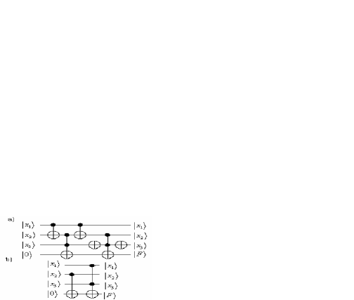
Figure 11: Implementaion of $F={\overline{x_{1}}x_{2}+x_{2}\overline{x_{3}}+x_{1}\overline{x_{2}}x_{3}}$ according to a) method [4], b) our method.

In another work [5] a method is described that requires auxiliary qubits in the quantum circuits obtained. In Fig. 12 we give a comparison of a circuit obtained by this method (Fig. 12(a)) and the equivalent, but much simpler, circuit obtained by the method proposed in this paper (Fig. 12(b)).

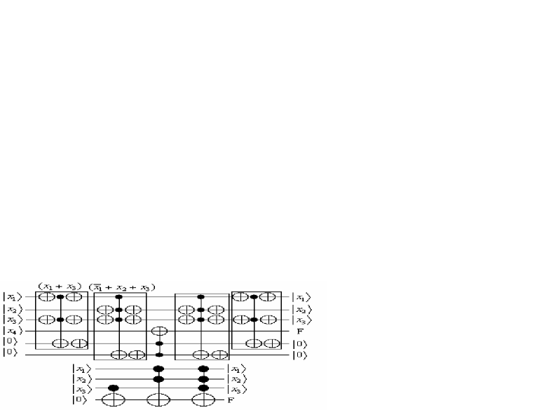
Figure 12: Implementaion of $F=(x_{1}+x_{3})(\overline{x_{1}}+x_{2}+x_{3})$ according to a) method [5], b) our method.

6 Reversible Version of Classical Operations

The construction of reversible classical Boolean circuits has received much attention [1, 7]. As a direct result from the 3-qubit quantum circuits shown in Fig.15 , we can pick a set of these circuits which represent the reversible version of the classical irreversible operations: AND, OR, NOT, NAND, NOR, XOR and XNOR . Using these versions of quantum circuits as reversible classical gates together with a reversible FAN-OUT version similar to that shown in [1] as shown in Table.4, we can build a classical non-quantum reversible version of any known digital circuits.

Using the gates shown in Table.4, we can build the reversible version of any digital circuit and apply the same methods of simplification and optimization applied on those kind of circuits (as shown in Fig.13). Of course this architecture need more investigation to estimate its efficiency.

Name	$\begin{array}[]{l}\mbox{Truth Table \par}\\ x_{1}x_{2}0\to x_{1}x_{2}F\end{array}$	Proof	Gate Black-Box
AND	$\begin{array}[]{l}000\to 000\\ 010\to 010\\ 100\to 100\\ 110\to 111\end{array}$	$\begin{array}[]{l}F=0\oplus x_{1}x_{2}\\ \,\,\,\,\,\,=x_{1}x_{2}\\ \end{array}$
OR	$\begin{array}[]{l}000\to 000\\ 010\to 011\\ 100\to 101\\ 110\to 111\end{array}$	$\begin{array}[]{l}F=0\oplus x_{1}x_{2}\oplus x_{1}\\ \,\,\,\,\,\,\,\,\,\,\oplus x_{2}\\ \,\,\,\,\,=x_{1}\overline{x_{2}}\oplus\overline{x_{2}}\oplus 1\\ \,\,\,\,\,=\overline{\overline{x_{1}}\,\,\overline{x_{2}}}\\ \,\,\,\,\,=x_{1}+x_{2}\end{array}$
NOT	$\begin{array}[]{l}0\to 1\\ 1\to 0\end{array}$

Table 4: Reversible version of irreversible classical gates.

Name	$\begin{array}[]{l}\mbox{Truth Table \par}\\ x_{1}x_{2}0\to x_{1}x_{2}F\end{array}$	Proof	Gate Black-Box
NAND	$\begin{array}[]{l}000\to 001\\ 010\to 011\\ 100\to 101\\ 110\to 110\end{array}$	$\begin{array}[]{l}F=\overline{0\oplus x_{1}x_{2}}\\ \,\,\,\,\,\,=\overline{x_{1}x_{2}}\end{array}$
NOR	$\begin{array}[]{l}000\to 001\\ 010\to 010\\ 100\to 100\\ 110\to 110\end{array}$	$\begin{array}[]{l}F=\overline{0\oplus x_{1}x_{2}\oplus x_{1}}\\ \,\,\,\,\,\,\,\,\overline{\oplus x_{2}}\\ \,\,\,\,\,=\overline{x_{1}\overline{x_{2}}\oplus\overline{x_{2}}\oplus 1}\\ \,\,\,\,\,=\overline{x_{1}}\overline{x_{2}}\\ \,\,\,\,\,=\overline{x_{1}+x_{2}}\end{array}$
FAN-OUT	$\begin{array}[]{l}00\to 00\\ 10\to 11\par\end{array}$	$0\oplus x=x$

Table 4: Continued…

Name	$\begin{array}[]{l}\mbox{Truth Table \par}\\ x_{1}x_{2}0\to x_{1}x_{2}F\end{array}$	Proof	Gate Black-Box
XOR	$\begin{array}[]{l}000\to 000\\ 010\to 011\\ 100\to 101\\ 110\to 110\end{array}$	$\begin{array}[]{l}0\oplus x_{1}\oplus x_{2}\\ =x_{1}\oplus x_{2}\end{array}$
XNOR	$\begin{array}[]{l}000\to 001\\ 010\to 010\\ 100\to 100\\ 110\to 111\end{array}$	$\begin{array}[]{l}\overline{0\oplus x_{1}\oplus x_{2}}\\ =\overline{x_{1}\oplus x_{2}}\\ \end{array}$

Table 4: Continued…

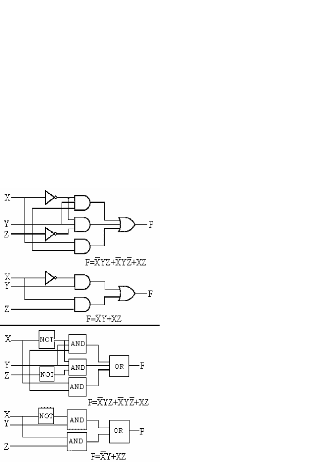
Figure 13: Converting digital circuits to it’s reversible version.

References

• [1] T. Toffoli (1980), Reversible Computing, Automata, Languages, and Programming, Springer-Verlag, pp. 632-644.
• [2] S. Devadas and A. Ghosh an K. Keutzer (1994), Logic Synthesis, McGraw–Hill.
• [3] A. Barenco, C. Bennett, R. Cleve, D. P. Divincenzo, N. Margolus, P. Shor, T. Sleator, J. Smolin and H. Weinfurter (1995), Elementary Gates for Quantum Computation, Phys. Rev. A, 52(5),pp. 3457-3467.
• [4] J. Lee, J. Kim, Y. Cheong and S. Lee (1999),A Practical Method for Constructing Quantum Combinational Logic Circuits, KPS 1999 Fall, Session Da (Poster, in Korean).
• [5] K. Iwama, Y. Kambayashi and S. Yamashita (2002), Transformation rules for Designing CNOT–based Quantum Circuits, Proceedings of the 39th Conference on Design Automation, ACM Press, pp. 419-424.
• [6] V. Shende, A. Prasad, I. Markov and J. Hayes (2002), Reversible Logic Circuit Synthesis, Proceedings of ACM/IEEE Intl. Conf. Comp.-Aided Design, pp. 353-360.
• [7] E. Fredkin and T. Toffoli (1982), Conservative Logic, International Journal of Theoretical Physics, 21,pp. 219-253.