Ground state entanglement in quantum spin chains

Abstract

A microscopic calculation of ground state entanglement for the XY and Heisenberg models shows the emergence of universal scaling behavior at quantum phase transitions. Entanglement is thus controlled by conformal symmetry. Away from the critical point, entanglement gets saturated by a mass scale. Results borrowed from conformal field theory imply irreversibility of entanglement loss along renormalization group trajectories. Entanglement does not saturate in higher dimensions which appears to limit the success of the density matrix renormalization group technique. A possible connection between majorization and renormalization group irreversibility emerges from our numerical analysis.

I Introduction

At zero temperature, the properties of a quantum many-body system are dictated by the structure of its ground state. The degree of complexity of this structure varies from system to system. It ranges from exceptionally simple cases –e.g. when an intense magnetic field aligns all the spins of a ferromagnet along its direction, producing a product or unentangled state– to more intricate situations where entanglement pervades the ground state of the system. Thus, entanglement appears naturally in low temperature quantum many-body physics, and it is at the core of relevant quantum phenomena, such as superconductivity BCS57 , quantum Hall effect La83 and quantum phase transitions sach99 .

There are several good reasons to study entanglement in quantum many-body systems. On the one hand, over the last decade entanglement has been realized to be a crucial resource to process and send information in novel ways BeDi00 . It is, for instance, the key ingredient in quantum information tasks such as quantum teleportation and superdense coding, and it also appears in most proposed algorithms for quantum computation book . This has triggered substantial experimental efforts to produce entanglement in engineered quantum systems FortPhys . Consequently, one may want to investigate and characterize entanglement in those systems where it appears in a natural way, with a view either to extract it to process quantum information or else to gain insight into physical mechanisms that can be used to entangle a large number of quantum systems.

But one can also motivate these studies without referring to potential applications of entanglement as a resource in quantum information processing. The ground state of a typical quantum many-body system consists of a superposition of a huge number of product states. Understanding this structure is equivalent to establishing how subsystems are interrelated, which in turn is what determines many of the relevant properties of the system. In this sense, the study of multipartite entanglement offers an attractive theoretical framework from which one may be able to go beyond customary approaches to the physics of quantum collective phenomena pres01 . Most promisingly, a theory of entanglement in quantum many-body systems may also lead to the development of new numerical techniques. In particular, recent results gvprep show how to efficiently simulate certain quantum systems through a suitable parametrization of quantum superpositions.

In this paper we present a quantitative analysis of entanglement in several one-dimensional spin models, expanding and complementing the results of Ref. vid02 . The models we discuss fulfill a convenient combination of requirements: they are solvable –the ground state can be computed by using well-known analytical and numerical techniques– and at the same time they successfully describe a rich spectrum of physical phenomena, which include ordered and disordered magnetic phases connected by a quantum phase transition sach99 . The paper has been divided into five more sections. A brief summary of them follows.

The study of entanglement in a system with many particles can be approached in several complementary ways vid02 ; NiTe ; W00 ; OW01 ; ved01 ; ved02 ; WFS01 ; WaZa02 ; Wa02 ; rest ; OsNi02 ; Os02 . In section II we briefly review some of them and explain the specific aspect on which we focus here. We consider a quantum spin chain in its ground state. Our aim is to determine the degree of entanglement between a block of spins and the rest of the chain, as measured by the von Neumann entropy of the block, and to investigate how this entanglement grows with the size of the block.

Sections III and IV are devoted, respectively, to computing the entropy of a spin block for the XY model and for the XXZ model. The calculation is divided into two parts. First, we need to construct the ground state of the spin chain, which for general chains is a highly non-trivial problem. Fortunately, the XY model can be treated analytically in the limit of an infinite chain Ann ; Kat ; Bar . Similarly, for the XXZ model there are known techniques bet01 ) to easily cope with chains consisting of up to twenty spins. Then, from the ground state of each model we extract the entropy of a spin block. For the XY model this is shown to build down to diagonalizing a matrix whose dimensions grow only quadratically with the size of the block. In this way we compute the entanglement for blocks of up to several hundreds of spins. In the XXZ model, instead, we only consider blocks of up to ten qubits, but the results can already be convincingly interpreted as an independent confirmation of the conclusions drawn from the XY model.

In section V we discuss the findings of the previous two sections, that can be summarized as follows:

• Off a critical point, the entanglement of a block of spins with the chain –a function that turns out to grow monotonically with the number of spins in the block– achieves a finite saturation value for sufficiently large blocks.

• At a quantum phase transition, instead, the entropy of a block of spins grows unboundedly. More specifically, the entropy for a critical chain grows logarithmically in the size of the spin block, with a multiplicative coefficient that depends only on the universality class of the phase transition. That is, at the critical point entanglement obeys a universal scaling law.

Interestingly, the behavior of the entanglement in a critical spin chain matches well-known results in conformal field theory, where the geometric entropy –analogous to the spin-block entropy, but defined in the continuum– has been computed for 1+1 dimensional theories Sr93 ; Ca94 ; Fi94 ; HoLaWi . The geometric entropy grows logarithmically with the size of the interval under consideration and with a multiplicative constant given by the central charge of the theory. As described in section VI, a consistent picture arises. At a critical point the large-scale behavior of a spin chain is universal, with the quantum phase transition belonging to a given universality class. All long-range properties of the chain are then described by the conformal field theory associated with that universality class. In particular the entanglement between a large block of spins and the rest of the chain follows the same law as the geometric entropy.

The above connection between entanglement and the geometric entropy of conformal theories has several implications. Previous calculations of the entropy in higher dimensions indicate that in 2- and 3-dimensional spin lattices the entropy of a spin block grows as the size of the boundary of the block —the same law holding both for critical and non-critical lattices. The lack of saturation of the entropy as a function of the size of the block explains the failure of the DMRG technique white . Thus, we interpret in terms of entanglement why this numerical technique —so successful for non-critical spin chains— deteriorates in critical one-dimensional lattices and fails to work properly both for critical and non-critical chains and in 2- and 3-dimensional lattices RO99 .

The scaling law obeyed by the entanglement of a critical ground state implies that the greater a spin block is, the more disordered or mixed its density matrix. Thus, the entropy indicates an ordering of the reduced density matrices, according to how mixed they are. This ordering can be further refined and shown to actually emerge from majorization relations between the reduced density matrices.

Finally, we translate the results related to the c-theorem zam86 to quantum information. Entanglement is argued to decrease along renormalization group trajectories. A number of numerical and analytical results are consistent with the idea that irreversibility of renormalization group flows may be rooted on a majorization ordering of the vacuum density matrices along the flow.

II Entanglement measures in a quantum spin chain

A major difficulty in studying the entanglement in a many-body quantum system comes from the fact that the number of degrees of freedom involved grows exponentially with the number of interacting subsystems. In particular, the task of computing explicitly the ground state of a chain consisting of a large number of spins, to then analyze its entanglement properties, turns out to be very difficult, if not insurmountable.

Fortunately, for some specific spin models the ground state has been previously computed. One can then try to characterize entanglement in these models. This is again a rather ambitious enterprise. On the one hand, it entails serious computational difficulties, since the corresponding ground states, when expressed in a local basis, still involve exponentially many coefficients. On the other hand such characterization is also challenging from a conceptual viewpoint. The study of entanglement of a large number of particles is a relatively unexplored subject and it has not yet even been established what aspects of a ground state a sensible characterization should consider. Therefore, an important part of the problem is to actually identify which quantities may be of interest.

This section is devoted to describe and motivate our particular approach, which attempts to characterize the ground state of the spin chain through the spectral properties of the reduced density matrix for a block of spins, and in particular through its entropy. We start by presenting some generalities and reviewing previous work.

II.1 Overview of previous work

A state $\mbox{$|\Psi\rangle$}\in{{\cal H}_{2}}^{\otimes N}$ of $N$ spins is entangled if it cannot be written as the tensor product of single-spin states,

$$\mbox{$|\Psi\rangle$}\neq\mbox{$|\psi_{1}\rangle$}\otimes\mbox{$|\psi_{2}\rangle$}\otimes\cdots\otimes\mbox{$|\psi_{N}\rangle$}.$$ (1)

Product states depend on ${\cal O}(N)$ parameters and are therefore just a subset of zero measure in the set of states of $N$ spins. A generic entangled state, when expressed in a local basis, depends on ${\cal O}(2^{N})$ parameters. Characterizing entanglement is about identifying a reduced subset of parameters that are particularly relevant from a physical or computational point of view.

II.1.1 Entanglement under local manipulation

In recent years a quantitative theory of bipartite entanglement has been developed. As proposed in the pioneering work by Bennett, Bernstein, Popescu and Schumacher benn01 , this theory is based on the possibility of converting one entangled state $|\Psi\rangle$ into another entangled state $|\Psi^{\prime}\rangle$ by applying local operations on each of the subsystems and communicating classically, a set of transformations denoted as LOCC (see qic for extensive reviews). The basic idea is that if the state $|\Psi\rangle$ can be converted into the state $|\Psi^{\prime}\rangle$ by LOCC,

$$\mbox{$|\Psi\rangle$}\longrightarrow\mbox{$|\Psi^{\prime}\rangle$}$$ (2)

then $|\Psi\rangle$ cannot be less entangled than $|\Psi^{\prime}\rangle$, since LOCC can only introduce classical correlations between the subsystems. Local convertibility can in this way be used to compare the amount of entanglement in different states.

Following these ideas two remarkably simple characterizations of pure-state entanglement are possible for systems with $N=2$ subsystems:

($i$) Bennett et al. benn01 showed that, in an asymptotic sense, any entangled state $\mbox{$|\Psi\rangle$}_{AB}$ of two particles $A$ and $B$ is equivalent (that is, reversibly convertible by LOCC) to some fraction $E(\Psi)$ of an EPR state,

$$\frac{1}{\sqrt{2}}(\mbox{$|0\rangle$}_{A}\otimes\mbox{$|0\rangle$}_{B}+\mbox{$|1\rangle$}_{A}\otimes\mbox{$|1\rangle$}_{B}).$$ (3)

Here the entropy of entanglement $E(\Psi)$ corresponds to the von Neumann entropy of the reduced density matrix $\rho_{A}\equiv{\rm tr}_{B}\mbox{$|\Psi\rangle\!\langle\Psi|$}$ for any one of the systems,

$$E(\Psi)\equiv-{\rm tr}(\rho_{A}\log_{2}\rho_{A}).$$ (4)

($ii$) Nielsen Nie subsequently showed that deterministic conversions of a single copy of $|\Psi\rangle$ into $|\Psi^{\prime}\rangle$ by LOCC are ruled by the majorization relation (to be introduced later in Eq. (17)). More general LOCC transformations are similarly ruled by a finite set of entanglement monotones mono .

The optimal local manipulation of a bipartite system in a pure state is presently well understood. Bipartite pure-state entanglement can be characterized by a single measure $E(\Psi)$ in the asymptotic regime and by a small set of entanglement monotones in the single-copy case. However, none of these results has been successfully generalized to systems with $N>2$ subsystems. In spite of the remarkable success achieved for bipartite systems, LOCC transformations do not seem to be a good a guidance to comprehensively characterize multipartite entanglement. Nevertheless, the above results can still be used to characterize any bipartite aspects of the entanglement in a multipartite system, and therefore will be sufficing for the purposes of this paper.

II.1.2 Entanglement in spin chains

The study of entanglement in condensed matter systems was initiated by Nielsen NiTe . He originally analyzed two interacting spins in the Heisenberg model with an external magnetic field and studied how entanglement depends on the temperature and the intensity of the spin-spin interaction and magnetic field. In his calculations, Nielsen used Wooters’ concurrence woo01 , a measure of mixed-state entanglement defined for two-qubit systems.

More recently, several other authors have also studied the concurrence in spin systems. Wooters W00 has studied the maximal nearest neighbor concurrence that an infinite, translationally invariant spin chain can have, a result extended by O’Connor and Wooters OW01 to finite spin rings. Furthermore, concurrence in the two-spin Heisenberg model has been reanalyzed by Arnesen, Bose and Vedral ved01 . Gunlycke, Bose, Kendon and Vedral ved02 have considered a ring of several spins with Ising interaction and external magnetic field, and studied how two-spin entanglement depended on the orientation of the magnetic field. Wang, Fu, Solomon WFS01 have studied the anisotropic Heisenberg model with three spins. For a Heisenberg ring of $N$ spins, Wang and Zanardi WaZa02 have expressed the nearest neighbor concurrence in terms of the internal energy of the ring and analyzed the violation of Bell inequalities, and Wang Wa02 has investigated the concurrence in the XX model. Ref. rest contains some other related works.

Osterloh, Amico, Falci and Fazio Os02 and Osborne and Nielsen OsNi02 have recently studied entanglement in the ground state of an infinite XY and Ising spin chains and its relation to quantum phase transitions. More specifically, they have computed the concurrence between pairs of spins, for different choices of the pair. For the Ising model with transverse magnetic field, the concurrence at nearest and next to nearest neighbors has a maximum near the critical point. Osterloh et al. have suggestively noticed that there seems to be some form of universal scaling in the derivative of the concurrence of nearest neighboring spins, and similarly for the second derivative of the next to nearest neighbors. A notable fact is that the concurrence seems to disappear at third nearest neighbors. As pointed out by Osborne and Nielsen, this can be interpreted in terms of the monogamy of entanglement Woo03 . In practice, it can also be understood as a shortcoming for using a two-qubit measure in order to capture the global distribution of entanglement along the chain.

II.2 Entropy of a block of spins

The approach we follow here has been proposed by Vidal, Latorre, Rico and Kitaev vid02 and, as previous works based on the concurrence, it is focussed on bipartite entanglement. But instead of analyzing the entanglement between two of the spins of the system, we consider a whole block of adjacent spins and study its entanglement with the rest of the chain. We are particularly interested in how the entanglement between the block and the chain depends on the size of the block. In this way, we expect to be able to explore the behavior of quantum correlations at different length scales and to capture the emergence of universal scaling at a quantum critical point. Later on in this section we will further motivate our choice by referring to the relationship between entanglement and the efficiency of numerical schemes for the simulation of spin chains.

Let $|\Psi_{g}\rangle$ denote the ground state of a chain of $N$ spins and let $\rho_{L}$,

$$\rho_{L}\equiv{\rm tr}_{N-L}\mbox{$|\Psi_{g}\rangle\!\langle\Psi_{g}|$},$$ (5)

be the reduced density matrix for $L$ contiguous spins. In the models we shall discuss, the ground state $|\Psi_{g}\rangle$ is translationally invariant, so that $\rho_{L}$ does not depend on the position of the block of spins but only on its size $L$. Because the chain is in a pure state, all the information about the entanglement between the block of spins and the rest of the chain is contained in the eigenvalues of $\rho_{L}$. If $\rho_{L}$ is a pure state itself, then the block is unentangled from the chain. Instead, if $\rho_{L}$ has many non-zero eigenvalues, this roughly indicates a lot of entanglement between the block and the chain. As a matter of fact, the whole spectrum Sp$(\rho_{L})$ is of interest, as we shall discuss shortly. For concreteness, however, we will mainly use a single function of the spectrum of $\rho_{L}$, namely the von Neumann entropy

$$S_{L}\equiv-{\rm tr}\left(\rho_{L}\log_{2}{\rho_{L}}\right),$$ (6)

as a measure of entanglement. This choice corresponds to the entropy of entanglement benn01 (recall Eq. (4)) between the block and the rest of the chain.

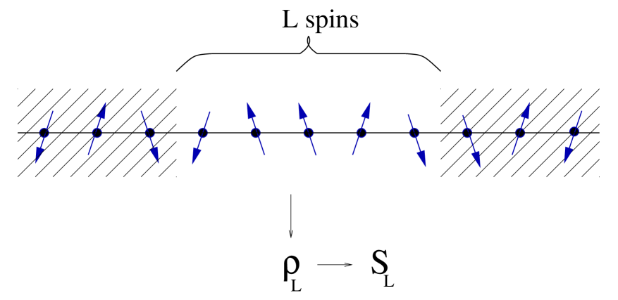
Figure 1: The entropy $S_{L}$ corresponds to the von Neumann entropy of the reduced density matrix $\rho_{L}$ for a block of $L$ adjacent spins, and measures the entanglement between the block and the rest of the chain. State $\rho_{L}$ is obtained from the ground state $|\Psi_{g}\rangle$ of the N spin chain by tracing out all $N-L$ spins outside the block.

II.2.1 Properties of the entropy of a block of spins

Let us discuss some general properties of $S_{L}$ as a function of $L$. $S_{L}$ is positive by construction,

$$S_{L}\geq 0,\leavevmode\nobreak\ \leavevmode\nobreak\ \leavevmode\nobreak\ \leavevmode\nobreak\ \leavevmode\nobreak\ L=0,1,\cdots,N,$$ (7)

where for convenience we define $S_{0}\equiv 0$. Because the chain is in a pure state $|\Psi_{g}\rangle$, the spectrum Sp($\rho_{L}$) of the reduced density matrix for a block of spins and the spectrum for the rest of the chain are the same. In particular, the two parts will also have the same entropy. Recalling that the ground state $|\Psi_{g}\rangle$ is translationally invariant, we have

$$S_{L}=S_{N-L},\leavevmode\nobreak\ \leavevmode\nobreak\ \leavevmode\nobreak\ \leavevmode\nobreak\ \leavevmode\nobreak\ L=0,1,\cdots,N.$$ (8)

In addition, $S_{L}$ is a concave function petz ,

$$S_{L}\geq\frac{S_{L-M}+S_{L+M}}{2},$$ (9)

where $L=0,\cdots,N,$ and $M=0,\cdots,\min\leavevmode\nobreak\ \{N\!-\!L,L\}$. This can be proved with the help of the strong subadditivity of the von Neumann entropy book ; lie01 ,

$$S(ABC)+S(B)\leq S(AB)+S(BC),$$ (10)

where $A$, $B$ and $C$ are three subsystems and, say, $S(AB)$ denotes the entropy of $\rho_{AB}$, the joint state of systems $A$ and $B$. Let $A$, $B$ and $C$ correspond to three adjacent blocks of our translational invariant spin chain, with $M$, $L\!-\!M$ and $M$ spins respectively. Then we have

$$S(ABC) = S_{L+M}$$ (11)

$$S(AB)=S(BC) = S_{L}$$ (12)

$$S(B) = S_{L-M},$$ (13)

and Eq. (10) reads

$$S_{L+M}+S_{L-M}\leq 2S_{L},$$ (14)

from where Eq. (9) follows.

Finally, we note that the above properties imply that $S_{L}$ does not decrease as a function of $L$ in the interval $L\in[0,N/2]$. In particular, in the limit of an infinite chain, $N\rightarrow\infty$, $S_{L}$ becomes a non-decreasing, concave function for all finite values of $L$.

II.2.2 Examples

It is possible to get extra insight into the properties of $S_{L}$ as a measure of entanglement by analyzing some particular cases, as illustrated in Fig. (2). We note first that $S_{L}$ is upper bounded by

$$S_{L}\leq\min\{L,N\!-\!L\},$$ (15)

since $\rho_{L}$ is supported in a local space of dimension $d_{L}=\min\{2^{L},2^{N-L}\}$, whereas $S_{L}$ vanishes for all $L$ only for product (i.e. unentangled) states.

The paradigmatic GHZ state of $N$ spins or qubits,

$$\frac{1}{\sqrt{2}}(\mbox{$|0\rangle$}^{\otimes N}+\mbox{$|1\rangle$}^{\otimes N}),$$ (16)

is often regarded as a maximally entangled state. However, from the present perspective it is only slightly entangled. Indeed, the entropies of a block of spins are $S_{L}=1$ for $L=1,\cdots,N\!-\!1$, and are therefore far below the upper bound (15).

Here we will be concerned with the ground state $|\Psi_{g}\rangle$ of spin chains that are invariant under discrete translations by any number of sites. [For finite chains, we will assume that the extremal spins are connected (spin rings) and will require invariance under circular translations.] One could expect that translational symmetry of $|\Psi_{g}\rangle$ implies a more restrictive bound for the values $S_{L}$ can achieve. However this is not the case, since Stelmachovic et al. ste01 have found a translationally invariant state that saturates (15). This is in contrast with the case of states that are invariant under all possible permutations of the spins. There the dimension $d_{L}^{\rm sym}=L+1$ of the symmetric subspace leads to the upper bound $S_{L}^{\rm sym}\leq\log_{2}L+1$.

Finally, at a critical point the ground state may have some extra symmetries. In particular, it is known that in the large scale limit (that is, for scales much larger than the distance between neighboring spins) a critical spin chain is conformal invariant. We will explore the implications of this additional symmetry in section VI. The ground state entropy for critical chains will turn out to grow as $S_{L}=k\log_{2}L$ for some universal constant $k$.

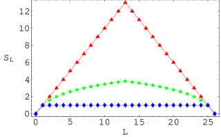
Figure 2: Bounds for the entropy $S_{L}$ for some pure states in a system with N=26 spins. Triangles correspond to the linear upper bound (15), and applies to translationally invariant states (and, more generally, to arbitrary $N$-qubit states). Stars are the logarithmic upper bound for a symmetric state under permutations. The diamonds are the values of the entropy for a GHZ state.

II.2.3 Majorization and von Neumann entropy

As mentioned above, the entanglement between a block of spins and the rest of the chain is a function of the spectrum Sp$(\rho_{L})$ of the reduced density matrix of the block. Our ultimate aim is to characterize how this entanglement depends on the number $L$ of spins in the block. A main motivation for this is that in this way we hope to capture the emergence of universal scaling for entanglement at a quantum phase transition. Therefore we would like to be able to compare the spectrum Sp($\rho_{L}$) for different values of $L$.

The entropy $S_{L}$ can be used for this purpose, for it establishes an order in the set of probability distributions –equivalently, in the set of spectra of density matrices. For instance, we have mentioned above that the entropy $S_{L}$ is non-decreasing in the interval $L\in[0,N/2]$. We can now use this result to say that, according to the entropy, the entanglement of a block of spins and the rest of the chain monotonically increases with the size of the block (for blocks smaller than half of the chain).

Nevertheless, there are other powerful tools to compare probability distributions, and by using them one may obtain a finer characterization of entanglement. In particular, a far more tight sense of (partial) ordering between probability distributions is established by the majorization relation Bh96 , a set of inequalities that control the conversion of bipartite entanglement by LOCC in the single-copy scenario Nie ; mono ; gui02 .

Let us briefly recall that a given probability distribution $x\equiv\{x_{i}\}$ (where $x_{1}\geq\cdots\geq x_{n}$) is majorized by another probability distribution $y\equiv\{y_{i}\}$ (where $y_{1}\geq\cdots\geq y_{n}$), denoted $x\prec y$, when the following series of inequalities are simultaneously fulfilled:

$$x_{1} \leq y_{1}$$

$$x_{1}+x_{2} \leq y_{1}+y_{2}$$

$$\vdots$$

$$x_{1}+x_{2}+\cdots+x_{n} = y_{1}+y_{2}+\cdots+y_{n}.$$ (17)

The majorization relation $x\prec y$ expresses the fact that $y$ is more ordered than $x$. Given two arbitrary probability distributions $x$ and $y$, inequalities (17) are not likely to be simultaneously fulfilled, but when they are, most measures of order are consistent with $x\prec y$. In particular, the von Neumann entropy fulfills

$$\rho\prec\rho^{\prime}\leavevmode\nobreak\ \Rightarrow\leavevmode\nobreak\ S(\rho)>S(\rho^{\prime}),$$ (18)

where $\rho\prec\rho^{\prime}$ refers to majorization between the spectra of these two density matrices.

In section VI we shall explore whether a majorization relation underlies the scaling behavior of the entropy $S_{L}$ at critical points.

II.3 Entanglement
in numerical studies of a quantum spin chain

There are many aspects of the ground state of a spin chain that could be taken as a guide to characterize its entanglement. Our choice can be motivated by the role the reduced density matrix $\rho_{L}$ of a block of spins plays in some numerical schemes. We finish this section by explaining how the spectrum Sp$(\rho_{L})$ of $\rho_{L}$ determines the efficiency of White’s density matrix renormalization group (DMRG) method white and of a recently proposed simulation scheme for the simulation of quantum spin chains gvprep .

White’s DMRG method white is a numerical technique that has brought an enormous progress in the study of one-dimensional quantum systems such as quantum spin chains. It allows to compute ground state energies and correlation functions with spectacular accuracy for non-critical spin chains. The DMRG method, however, loses its grip (as many other methods) near a critical point and fails to work for quantum spin lattices in two or three dimensions even away from the critical point RO99 . As recently explained by Osborne and Nielsen niel01 in the language of quantum information, the degree of performance of this method is directly related to the way it accounts for entanglement.

Let us consider a large spin chain and its ground state $|\Psi_{g}\rangle$. The DMRG method is based on computing properties of $|\Psi_{g}\rangle$ by constructing an approximation to the reduced density matrix $\rho_{L}$ for a block of $L$ spins, for an increasing value of $L$. This is done by retaining only the relevant degrees of freedom of the Hilbert space associated to the block of spins. Such degrees of freedom are given by the eigenvectors of $\rho_{L}$ with greatest weights or eigenvalues $\{p_{L}^{i}\}$, that we assume decreasingly ordered, $p_{L}^{i}\geq p_{L}^{i+1}$  $(i=1,\cdots,2^{N}\!\!-\!1)$.

Notice that the spectrum Sp($\rho_{L}$) typically contains as many as $2^{N}$ relevant eigenvalues, in which case the computational cost of the DMRG method explodes as the block size $L$ grows. However, not all eigenvalues have the same weight, and a good approximation to $\rho_{L}$ may be significantly cheaper to achieve than the exact reduced density matrix. Let $\raisebox{1.29167pt}{$\chi$}_{L}^{\epsilon}$ denote the number of eigenvalues such that

$$\sum_{i=1}^{\raisebox{0.90417pt}{$\chi$}_{L}^{\epsilon}}p_{L}^{i}\geq 1-\epsilon,\leavevmode\nobreak\ \leavevmode\nobreak\ \leavevmode\nobreak\ \leavevmode\nobreak\ \leavevmode\nobreak\ \leavevmode\nobreak\ 0\leq\epsilon\ll 1.$$ (19)

That is, $\raisebox{1.29167pt}{$\chi$}_{L}^{\epsilon}$ is an effective rank of $\rho_{L}$, resulting from ignoring all the smallest eigenvalues that sum up less than $\epsilon$. Then, if we are willing to accept a degree of accuracy $\epsilon$, the DMRG method need only retain $\raisebox{1.29167pt}{$\chi$}_{L}^{\epsilon}$ eigenvectors of $\rho_{L}$.

The efficiency of the DMRG depends on how small $\raisebox{1.29167pt}{$\chi$}_{L}^{\epsilon}$ is. In turn, $\raisebox{1.29167pt}{$\chi$}_{L}^{\epsilon}$ depends on how fast the eigenvalues $p_{L}^{i}$ decay with $i$ or, relatedly, on the entanglement between the block of spins and the rest of the chain. A very spread spectrum, roughly equivalent to a lot of entanglement, translates into a large $\raisebox{1.29167pt}{$\chi$}_{L}^{\epsilon}$ and a large computational cost. If, instead, the eigenvalues $\{p_{L}^{i}\}$ decay very fast with $i$, implying that there is not much entanglement, then $\raisebox{1.29167pt}{$\chi$}_{L}^{\epsilon}$ is small and so is the computational cost of the DMRG method.

Therefore, by studying the spectrum of $\rho_{L}$, and in particular the effective rank $\raisebox{1.29167pt}{$\chi$}_{L}^{\epsilon}$, we may be able to assess how well the DMRG will perform for given values of the parameters (external magnetic field, spin-spin interaction) defining a particular spin model.

On the other hand the effective rank $\raisebox{1.29167pt}{$\chi$}_{L}^{\epsilon}$ appears also as a decisive parameter in a recently proposed numerical scheme for the classical simulation of quantum spin chains gvprep . In this scheme the cost of the simulation is linear in the number $N$ of spins in the chain and grows as a small polynomial in $\raisebox{1.29167pt}{$\chi$}^{\epsilon}$,

$$\raisebox{1.29167pt}{$\chi$}^{\epsilon}\equiv\max_{L}\raisebox{1.29167pt}{$\chi$}_{L}^{\epsilon},$$ (20)

that is, polynomial in the maximal effective rank achieved for blocks of adjacent spins.

Summarizing, the spectrum of $\rho_{L}$, through the effective rank $\raisebox{1.29167pt}{$\chi$}_{L}^{\epsilon}$, is of direct interest for the numerical study of spin chains. The entropy $S_{L}$ of $\rho_{L}$ is related to the effective rank of $\rho_{L}$. Indeed, we have

$$\raisebox{1.29167pt}{$\chi$}_{L}^{\epsilon\rightarrow 0}\geq 2^{S_{L}}.$$ (21)

In addition, numerical evidence in spin chains indicates that $2^{S_{L}}$ also gives a rough estimate of $\raisebox{1.29167pt}{$\chi$}_{L}^{\epsilon}$ for small $\epsilon>0$.

In section V we shall discuss the results we have obtained for the entropy $S_{L}$, both for critical and non-critical spin chains, and analogous results for spin lattices. We will conclude that the degree of performance of the DMRG method for spin systems depends on how the entanglement between a block of spins and the rest of the system scales with the size of the block.

Note added: after completing the present work we have become aware of a number of contributions by Peschel et al Pes that study the spectrum of the reduced density matrix $\rho_{L}$ also with a view to assess the performance of the DMRG.

III XY model

In this section we study the entanglement of an infinite XY spin chain. We start by reviewing the main features of the XY model and by identifying some of the critical regions in the space of parameters that define the model. Then, we proceed to compute the ground state $|\Psi_{g}\rangle$ of the system, from which we obtain the reduced density matrix $\rho_{L}$ for $L$ contiguous spins. The knowledge of the eigenvalues of $\rho_{L}$ allows us to compute its entropy $S_{L}$ and, therefore, have a quantification of entanglement in spin chains. Further information contained in the eigenvalues of the density matrix will be explored in section VI.

The calculations of the spectrum and ground state of the XY model that appear in this section and in the appendices review previous work in spin chains. Lieb, Schultz and Mattis Ann solved exactly the XY model without magnetic field; Katsura Kat computed the spectrum of the XY model with magnetic field; Barouch and McCoy Bar obtained the correlation function for this model. Finally, the entropy $S_{L}$ was computed by Vidal, Latorre, Rico and Kitaev vid02 . Here we shall present an expanded version of this computation.

III.1 The XY Hamiltonian

The XY model consists of a chain of $N$ spins with nearest neighbor interactions and an external magnetic field, as given by the Hamiltonian

$$H_{XY}=-\frac{1}{2}\!\sum_{l}\left(\frac{1\!+\!\gamma}{2}\sigma_{l}^{x}\sigma_{l+1}^{x}+\frac{1\!-\!\gamma}{2}\sigma_{l}^{y}\sigma_{l+1}^{y}+\lambda\sigma_{l}^{z}\right).$$ (22)

Here $l$ labels the $N$ spins, $\sigma_{l}^{\mu}$ $(\mu=x,y,z)$ are the Pauli matrices,

$$\sigma^{x}=\left(\begin{array}[]{cc}0&1\\ 1&0\end{array}\right),\leavevmode\nobreak\ \sigma^{y}=\left(\begin{array}[]{cc}0&-i\\ i&0\end{array}\right),\leavevmode\nobreak\ \sigma^{z}=\left(\begin{array}[]{cc}1&0\\ 0&-1\end{array}\right),$$ (23)

acting on spin $l$, with

$$[\sigma_{l}^{\mu},\sigma_{m}^{\nu}]=2i\delta_{lm}\sum_{\tau=x,y,z}\epsilon_{\mu\nu\tau}\sigma_{l}^{\tau},$$ (24)

whereas parameter $\lambda$ is the intensity of the magnetic field, applied in the $z$ direction, and parameter $\gamma$ determines the degree of anisotropy of spin-spin interaction, which is restricted to the $xy$ plane in spin space.

The XY model encompasses two other well-known spin models. If the interaction is restricted to the $x$ direction in spin space, that is $\gamma=1$, then $H_{XY}$ turns into the Ising Hamiltonian with transverse magnetic field,

$$H_{\rm Ising}=-\frac{1}{2}\!\sum_{l}\left(\sigma_{l}^{x}\sigma_{l+1}^{x}+\lambda\sigma_{l}^{z}\right).$$ (25)

If, instead, we consider the interaction to be isotropic in the $xy$ plane, $\gamma=0$, then we recover the XX Hamiltonian with transverse magnetic field,

$$H_{XX}=-\frac{1}{2}\!\sum_{l}\left(\frac{1}{2}[\sigma_{l}^{x}\sigma_{l+1}^{x}+\sigma_{l}^{y}\sigma_{l+1}^{y}]+\lambda\sigma_{l}^{z}\right).$$ (26)

We note that these Hamiltonians are used to model the physics of one dimensional arrays of spins, but also to describe other quantum phenomena. For instance, the XX Hamiltonian corresponds to a particular limit of the boson Hubbard model

$$H_{B}=\sum_{l}\left(-w[\bar{a}_{l}^{\dagger}\bar{a}_{l+1}+\bar{a}_{l}^{\dagger}\bar{a}_{l+1}]-\mu n_{l}+\frac{U}{2}n_{l}(n_{l}-1)\right),$$

where $\bar{a}$ are bosonic annihilation operators,

$$[\bar{a}_{l},\bar{a}_{m}^{\dagger}]=\delta_{lm},$$ (27)

and $n_{l}\equiv\bar{a}_{l}^{\dagger}\bar{a}_{l}$ are number operators. The boson Hubbard model (see chapters 10 and 11 of sach99 ) consists of spinless bosons on $N$ sites, representing, say, Cooper pairs of electrons undergoing Josephson tunneling between superconducting islands or helium atoms moving on a substrate. The first term in $H_{B}$, proportional to $w$, allows hopping of bosons from site to site. The second term determines the total number of bosons in the model, with $\mu$ the chemical potential. The last term, with $U>0$, is a repulsive on-site interaction between bosons. Now, in the limit of large $U$, no more than 1 boson will be present at each site. Thus, each of the $N$ sites has an effective two-dimensional local space, and the identification

$$\sigma^{x}_{l} = \bar{a}_{l}+\bar{a}_{l}^{\dagger},$$ (28)

$$\sigma^{y}_{l} = -i(\bar{a}_{l}-\bar{a}_{l}^{\dagger}),$$ (29)

$$\sigma^{z}_{l} = 1-2\bar{a}_{l}^{\dagger}\bar{a}_{l},$$ (30)

takes $H_{B}$ into

$$H_{B}^{U\rightarrow\infty}=-\!\sum_{l}\left(\frac{w}{2}[\sigma_{l}^{x}\sigma_{l+1}^{x}+\sigma_{l}^{y}\sigma_{l+1}^{y}]-\frac{\mu}{2}\sigma_{l}^{z}\right),$$ (31)

which is the Hamiltonian of the XX spin chain model with transverse magnetic field of Eq (26).

III.2 Spectrum of $H_{XY}$ and critical properties

In appendix A we show that the spectrum of Hamiltonian $H_{XY}$ in Eq. (22) is given, in the limit of large $N$, by

$$\Lambda_{\phi}=\sqrt{(\lambda-\cos{\phi})^{2}+\gamma^{2}\sin^{2}{\phi}},$$ (32)

where $\phi\in[-\pi,\pi]$ is a label in momentum space. This result was obtained by Katsura Kat .

We can use the explicit expression (32) of $\Lambda_{\phi}$ to discuss the appearance of critical behavior in the XY model as a function of parameters $(\gamma,\lambda)$.

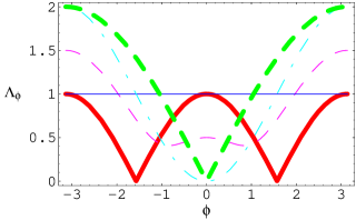
Figure 3: Energy of the system for different values of the parameters $\lambda$ and $\gamma$ as a function of $\phi$. The thick plot corresponds to the XX model without magnetic field, the dashed one to a system with $\lambda=\gamma=0.5$, the flat one is the Ising limit without magnetic field and the dot-dashed one and the thick dashed plot correspond to the isotropic and Ising model with $\lambda=1$, respectively.

The correlation length $\xi$ characterizes the exponential decay of correlations in the spin chain hen01 ; chak01 ,

$$\mbox{$\langle\sigma^{a}_{l}\sigma^{b}_{l+L}\rangle$}-\mbox{$\langle\sigma^{a}_{l}\rangle$}\mbox{$\langle\sigma^{b}_{l+L}\rangle$}\sim\exp(-L/\xi),$$ (33)

whereas the low energy dispersion $\Delta$ is given by

$$\Delta\equiv\Lambda_{\phi=0}.$$ (34)

The critical scaling of these two quantities is characterized in terms of $|\lambda-\lambda_{c}|$ (deviation from the critical magnetic field $\lambda_{c}$) and critical exponents $\nu$ and $s$ through

$$\begin{split}&\xi\sim|\lambda-\lambda_{c}|^{-\nu},\\ &\Delta\sim|\lambda-\lambda_{c}|^{s}.\end{split}$$ (35)

In addition, the dynamical critical behavior is given by the energy dispersion,

$$\Lambda_{\phi\to 0}\sim\phi^{z}(1+(\phi\xi)^{-z}),$$ (36)

where $z$ is the dynamical exponent. An analysis of the scaling phenomena gives the following useful relation between the critical exponents: $z=s/\nu$.

For $\lambda=1$ and any value of the anisotropy $\gamma\in[0,1]$, the spectrum $\Lambda_{\phi}$ in Eq. (32) has no mass gap, $\Delta=0$, and the spin chain is critical, so that $\lambda_{c}=1$. As far as criticality is concerned, we need to distinguish two cases depending on the anisotropy $\gamma$.

($i$) For $\gamma\in(0,1]$, Eq. (32) implies that the behavior for the energy dispersions are

$$\begin{split}\Delta&=\Lambda_{\phi=0}=|\lambda-1|,\\ \Lambda_{\phi\to 0}&\sim\sqrt{(\lambda-1)^{2}+(\gamma^{2}+1-\lambda)\phi^{2}}\\ &\sim\phi\left(1+\frac{|\lambda-1|}{\phi}\right).\end{split}$$ (37)

At the critical point $\lambda_{c}=1$, we find the critical exponents $z=1$ and $s=1$, whereas the divergence of the correlation length in this interval is

$$\xi=\frac{1}{|\lambda-1|},$$ (38)

with a critical exponent $\nu=1$. For later reference, we state that in this case the quantum spin chain belongs to the same universality class as the classical Ising model in two dimensions (or quantum Ising model in one dimension). The critical behavior in this class is described by the conformal field theory of a free massless fermion in 1+1 dimensions, with central charge equal to 1/2.

($ii$) For the case $\gamma=0$, we have

$$\Lambda_{\phi}=|\lambda-\cos{\phi}|$$ (39)

and the long wave dispersion and the energy dispersion are

$$\begin{split}\Delta&=\Lambda_{\phi=0}=|\lambda-1|,\\ \Lambda_{\phi\to 0}&\sim|\lambda-1+\phi^{2}/2|\\ &\sim\phi^{2}\left|1+\frac{\lambda-1}{\phi^{2}}\right|.\end{split}$$ (40)

Therefore the critical point $\lambda_{c}=1$ leads to the critical exponent $z=2$ and $s=1$ and the divergence of the correlation length in this interval is

$$\xi=\frac{1}{\sqrt{\lambda-1}},$$ (41)

with a critical exponent $\nu=\frac{1}{2}$. Notice, however, that in this case the spectrum $\Lambda_{\phi}$ is gapless for any $\lambda\in[0,1]$, since $\Lambda_{\phi}$ continuously vanishes for $\phi=\arccos(\lambda)$. This implies that the spin chain is actually critical for any value $\lambda\in[0,1]$ of the magnetic field. Again for later reference, we mention that in this case the quantum spin chain belongs to the universality class described by a free massless boson in 1+1 dimensions. This conformal theory has central charge equal to 1.

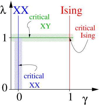
Figure 4: Some critical regions in the parameter space ($\gamma,\lambda$) for the XY model. The Ising model, $\gamma=1$, has a critical point at $\lambda=1$. The XX model, $\gamma=0$, is critical in the interval $\lambda\in[0,1]$. The whole line $\lambda=1$ is also critical. A complete analysis of the critical regions in this model was done by Barouch and McCoy in Bar

Summarizing, by analyzing the spectrum of $H_{XY}$ one finds two distinct critical regions in the parameter space $(\gamma,\lambda)$, namely the line $\lambda_{c}=1$ and the segment $(\gamma,\lambda)=(1,[0,1])$. The critical XX model corresponds to an unstable fixed point with respect to the anisotropy $\gamma$. If we depart from $(\gamma,\lambda)=(0,1)$ by a small perturbation $\gamma\neq 0$, the critical behavior of the spin chain turns from the universality class of the $XX$ model into that of the Ising model.

III.3 The ground state

We now turn to determine the ground state $|\Psi_{g}\rangle$ of the XY model with open boundary conditions,

$$H_{XY} = -\frac{1}{2}\!\sum_{l=-\frac{N-1}{2}}^{\frac{N-1}{2}}\left(\frac{1\!+\!\gamma}{2}\sigma_{l}^{x}\sigma_{l+1}^{x}+\frac{1\!-\!\gamma}{2}\sigma_{l}^{y}\sigma_{l+1}^{y}\right)$$ (42)

$$- \frac{1}{2}\sum_{l=-\frac{N-1}{2}}^{\frac{N-1}{2}}\lambda\sigma_{l}^{z},$$

in the limiting case of an infinite chain, $N\rightarrow\infty$.

Through a Jordan-Wigner transformation, Hamiltonian $H_{XY}$ can be cast into a quadratic form of fermionic operators, which in turn can be diagonalized by means of two additional canonical transformations, namely a Fourier transformation and a Bogoliubov transformation (see Appendix A for details). Next we will determine the ground state $|\Psi_{g}\rangle$ through a more convenient —although essentially equivalent— procedure that uses Majorana operators instead of fermionic operators.

The present calculation was sketched in vid02 and uses the formalism described in kit . Originally, the ground state of the XY model was determined by Lieb, Schultz and Mattis Ann in the case of no magnetic field, and by Barouch and McCoy Bar in the case of magnetic field.

Figure 5: This road map describes the steps followed in order to obtain the entropy $S_{L}$ of $L$ contiguous spins from an infinite $XY$ chain. We diagonalize the Hamiltonian $H_{XY}$ by rewriting it first in terms of Majorana operators $\check{a}$ and then in terms of Majorana operators $\check{b}$. The ground state $|\Psi_{g}\rangle$ is characterized by a correlation matrix $\Gamma^{B}$ for operators $\check{b}$, $\Gamma^{A}$ for operators $\check{a}$. Correlation matrix $\Gamma^{A}_{L}$ describes the reduced density matrix $\rho_{L}$ for a block of $L$ spins. $S_{L}$ is finally obtained from $\Gamma_{L}^{C}$, the block-diagonal form of $\Gamma_{L}^{A}$.

III.3.1 Majorana operators

For each site $l$ of the $N$-spin chain, we consider two Majorana operators, $\check{a}_{2l-1}$ and $\check{a}_{2l}$, defined by

$$\check{a}_{2l-1}\equiv\left(\prod_{m<l}\sigma_{m}^{z}\right)\sigma_{l}^{x};\leavevmode\nobreak\ \leavevmode\nobreak\ \leavevmode\nobreak\ \check{a}_{2l}\equiv\left(\prod_{m<l}\sigma_{m}^{z}\right)\sigma_{l}^{y}.$$ (43)

Operators $\check{a}_{m}$ are Hermitian and obey anti-commutation relations,

$$\check{a}_{m}^{\dagger}=\check{a}_{m},\leavevmode\nobreak\ \leavevmode\nobreak\ \leavevmode\nobreak\ \leavevmode\nobreak\ \leavevmode\nobreak\ \leavevmode\nobreak\ \{\check{a}_{m},\check{a}_{n}\}=2\delta_{mn}.$$ (44)

The change of variables of Eq. (43), parallel to the Jordan-Wigner transformation described in Appendix A, implies

$$\check{a}_{2l}\check{a}_{2l+1} = \sigma_{l}^{y}\sigma_{l}^{z}\sigma_{l+1}^{x}=i\sigma_{l}^{x}\sigma_{l+1}^{x},$$ (45)

$$\check{a}_{2l-1}\check{a}_{2l+2} = \sigma_{l}^{x}\sigma_{l}^{z}\sigma_{l+1}^{y}=-i\sigma_{l}^{y}\sigma_{l+1}^{y},$$ (46)

$$\check{a}_{2l-1}\check{a}_{2l} = \sigma_{l}^{x}\sigma_{l}^{y}=i\sigma_{l}^{z},$$ (47)

so that Hamiltonian $H_{XY}$ becomes

$$H_{XY} = \frac{i}{2}\sum_{l=-\frac{N-1}{2}}^{\frac{N-1}{2}}\left(\leavevmode\nobreak\ \frac{1+\gamma}{2}\leavevmode\nobreak\ \check{a}_{2l}\check{a}_{2l+1}-\frac{1-\gamma}{2}\leavevmode\nobreak\ \check{a}_{2l-1}\check{a}_{2l+2}\leavevmode\nobreak\ \right)$$ (48)

$$+ \frac{i}{2}\sum_{l=-\frac{N-1}{2}}^{\frac{N-1}{2}}\lambda\check{a}_{2l-1}\check{a}_{2l}\leavevmode\nobreak\ ,$$

or, equivalently,

$$H_{XY}=\frac{i}{4}\sum_{m,n=-N}^{N-1}A_{mn}\check{a}_{m}\check{a}_{n},$$ (49)

where $A$ is a real, skew-symmetric matrix given by

$$A=\left[\begin{array}[]{cccccc}A_{0}&A_{1}&&&\\ -A_{1}^{T}&A_{0}&A_{1}&&\\ &&\ddots&&\\ &&-A_{1}^{T}&A_{0}&A_{1}\\ &&&-A_{1}^{T}&A_{0}\\ \end{array}\right],$$ (50)

and

$$A_{0}=\left[\begin{array}[]{cc}0&2\lambda\\ -2\lambda&0\end{array}\right],\leavevmode\nobreak\ \leavevmode\nobreak\ A_{1}=\left[\begin{array}[]{cc}0&-(1\!-\!\gamma)\\ 1\!+\!\gamma&0\end{array}\right].$$ (51)

Figure 6: Through transformation (43), we can associate two Majorana operators, $\check{a}_{2l-1}$ and $\check{a}_{2l}$, to site $l$ of the spin chain. Notice, however, the non-local character of such transformation: $\check{a}_{2l-1}$ and $\check{a}_{2l}$ are a product of Pauli matrices from sites $-(N-1)/2$ to $l$.

Let $W\in SO(2N)$ be a special orthogonal matrix that brings $A$ into its block diagonal form $B=WAW^{T}$,

$$B=\bigoplus_{k=-\frac{N-1}{2}}^{\frac{N-1}{2}}\tilde{\Lambda}_{k}\left[\begin{array}[]{cc}0&1\\ -1&0\end{array}\right],$$ (52)

and let

$$\check{b}_{p}=\sum_{m=-N}^{N-1}W_{pm}\check{a}_{m},\leavevmode\nobreak\ \leavevmode\nobreak\ \leavevmode\nobreak\ -N+1\leq p\leq N,$$ (53)

be a new set of Majorana operators,

$$\check{b}_{p}^{\dagger}=\check{b}_{p},\leavevmode\nobreak\ \leavevmode\nobreak\ \leavevmode\nobreak\ \leavevmode\nobreak\ \leavevmode\nobreak\ \leavevmode\nobreak\ \{\check{b}_{p},\check{b}_{q}\}=2\delta_{pq}.$$ (54)

The canonical transformation induced by $W$ is parallel to the Fourier and Bogoliubov transformations for fermionic operators that appear in Appendix A, where also an explicit expression for $\tilde{\Lambda}_{k}$ is displayed. In terms of operators $\check{b}$, $H_{XY}$ reads

$$H_{XY} = \frac{i}{4}\sum_{p,q=-N}^{N-1}B_{pq}\check{b}_{p}\check{b}_{q}$$ (55)

$$= \frac{i}{4}\sum_{k=-\frac{N-1}{2}}^{\frac{N-1}{2}}\tilde{\Lambda}_{k}(\check{b}_{2k-1}\check{b}_{2k}-\check{b}_{2k}\check{b}_{2k-1}).$$ (56)

III.3.2 Correlation matrix

The diagonalization of $H_{XY}$ essentially concludes with the determination of the explicit form of matrix $W$, as presented in Appendix B. However, in order to analyze the resulting ground state $|\Psi_{g}\rangle$, it is convenient to momentarily switch to the more familiar language of fermionic operators. We define a set of $N$ spinless fermionic operators $\hat{b}$,

$$\hat{b}_{k}\equiv\frac{\check{b}_{2k-1}+i\check{b}_{2k}}{2},$$ (57)

$-(N-1)/2\leq k\leq(N-1)/2$, obeying the anticommutation relations

$$\{\hat{b}^{\dagger}_{k},\hat{b}_{p}\}=\delta_{kp},\leavevmode\nobreak\ \leavevmode\nobreak\ \leavevmode\nobreak\ \{\hat{b}_{k},\hat{b}_{p}\}=0,$$ (58)

in terms of which Hamiltonian $H_{XY}$ becomes, up to an irrelevant constant,

$$H_{XY}=\sum_{k=-\frac{N-1}{2}}^{\frac{N-1}{2}}\tilde{\Lambda}_{k}\hat{b}_{k}^{\dagger}\hat{b}_{k}.$$ (59)

The ground state of $H_{XY}$ is annhilated by all $\hat{b}$,

$$\hat{b}_{k}\mbox{$|\Psi_{g}\rangle$}=0,$$ (60)

so that $\mbox{$\langle\Psi_{g}|$}\hat{b}_{k}^{\dagger}\hat{b}_{k}\mbox{$|\Psi_{g}\rangle$}$ —that is, the expectation value of a positive operator— vanishes and $\mbox{$\langle\Psi_{g}|$}H_{XY}\mbox{$|\Psi_{g}\rangle$}=0$ corresponds to the smallest eigenvalue of $H_{XY}$. Then, since $\hat{b}_{k}^{\dagger}\hat{b}_{k}+\hat{b}_{k}\hat{b}_{k}^{\dagger}=I$ and $\hat{b}_{k}^{\dagger}\hat{b}_{k}\mbox{$|\Psi_{g}\rangle$}=0$, we also have

$$\hat{b}_{k}\hat{b}_{k}^{\dagger}\mbox{$|\Psi_{g}\rangle$}=\mbox{$|\Psi_{g}\rangle$}.$$ (61)

Let $\langle M\rangle$ denote the expectation value $\mbox{$\langle\Psi_{g}|$}M\mbox{$|\Psi_{g}\rangle$}$ for operator $M$. We readily have

$$\langle\hat{b}_{k}\rangle = 0,$$ (62)

$$\langle\hat{b}_{k}\hat{b}_{p}\rangle = 0,$$ (63)

$$\langle\hat{b}_{k}\hat{b}_{p}^{\dagger}\rangle = \delta_{kp}.$$ (64)

More generally, Wick’s theorem establishes that any non-vanishing expectation value corresponding to a product of operators $\hat{b}$ and $\hat{b}^{\dagger}$ can be expressed in terms of $\langle\hat{b}_{k}\hat{b}_{p}^{\dagger}\rangle$ and $\langle\hat{b}_{k}\hat{b}_{p}\rangle$ and their complex conjugates. For instance, we have

$$\langle\hat{b}_{k_{1}}\hat{b}_{k_{2}}\hat{b}^{\dagger}_{k_{3}}\hat{b}^{\dagger}_{k_{4}}\rangle = \mbox{$\langle\hat{b}_{k_{1}}\hat{b}_{k_{2}}\rangle$}\mbox{$\langle\hat{b}^{\dagger}_{k_{3}}\hat{b}^{\dagger}_{k_{4}}\rangle$}-\mbox{$\langle\hat{b}_{k_{1}}\hat{b}^{\dagger}_{k_{3}}\rangle$}\mbox{$\langle\hat{b}_{k_{2}}\hat{b}^{\dagger}_{k_{4}}\rangle$}$$ (65)

$$+ \mbox{$\langle\hat{b}_{k_{1}}\hat{b}^{\dagger}_{k_{4}}\rangle$}\mbox{$\langle\hat{b}_{k_{2}}\hat{b}^{\dagger}_{k_{3}}\rangle$}.$$

This means that $|\Psi_{g}\rangle$ is a gaussian state, completely characterized by the expectation values of the first and second moments, Eqs. (62)-(64).

We can now return to the Majorana operators $\check{b}$. An equivalent characterization of $|\Psi_{g}\rangle$ is given in terms of the correlation matrix $\mbox{$\langle\check{b}_{p}\check{b}_{q}\rangle$}=\delta_{pq}+i\Gamma^{B}_{pq}$, where

$$\Gamma^{B}=\bigoplus_{k=-\frac{N-1}{2}}^{\frac{N-1}{2}}\left[\begin{array}[]{rc}0&1\\ -1&0\end{array}\right].$$ (66)

As direct substitution shows, $\Gamma^{B}$ amounts for both the expectation values $\langle\hat{b}_{k}\hat{b}_{p}^{\dagger}\rangle$ and $\langle\hat{b}_{k}\hat{b}_{p}\rangle$ simultaneously, which is the ultimate reason to conduct the present derivation in terms of Majorana operators.

Finally, we use $\Gamma^{B}$ to obtain the correlation matrix $\mbox{$\langle\check{a}_{m}\check{a}_{n}\rangle$}=\delta_{m,n}+i\Gamma^{A}_{mn}$ of the original Majorana operators $\check{a}$, where $\Gamma^{A}=W^{T}\Gamma^{B}W$. As shown in Appendix B, one obtains

$$\Gamma^{A}=\left[\begin{array}[]{ccccc}\Pi_{0}&\Pi_{1}&\cdots&\Pi_{N-1}\\ -\Pi_{1}&\Pi_{0}&&\vdots\\ \vdots&&\ddots&\vdots\\ -\Pi_{N-1}&\cdots&\cdots&\Pi_{0}\end{array}\right],\leavevmode\nobreak\ \leavevmode\nobreak\ \leavevmode\nobreak\ \Pi_{l}=\left[\begin{array}[]{cc}0&g_{l}\\ -g_{-l}&0\end{array}\right],$$ (67)

with real coefficients $g_{l}$ as given, in the limit of an infinite chain, $N\rightarrow\infty$, by

$$g_{l}=\frac{1}{2\pi}\int_{0}^{2\pi}d\phi e^{-il\phi}\frac{\cos\phi-\lambda-i\gamma\sin\phi}{|\cos\phi-\lambda-i\gamma\sin\phi|}.$$ (68)

We conclude that Eqs. (67)-(68) contain a complete characterization of the ground state $|\Psi_{g}\rangle$ of $H_{XY}$.

III.4 Entropy of a block of spins

The entropy of the reduced density matrix $\rho$ for $L$ adjacent spins,

$$S_{L}=-{\rm tr}(\rho\log_{2}\rho),$$ (69)

can be computed from $\Gamma^{A}$, Eq. (67), as follows.

In the limit of an infinite chain, the middle of the chain is fully translational invariant, in that the same $\rho_{L}$ describes the state of any block of $L$ contiguous spins. For notational convenience we choose the block to contain qubits $l=1,\cdots,L$. We can expand the density matrix $\rho_{L}$ of the block as

$$\rho_{L}=2^{-L}\!\!\!\!\!\!\!\!\!\!\sum_{\mu_{1},\cdots,\mu_{L}=0,x,y,z}\!\!\!\rho_{\mu_{1}\cdots\mu_{L}}\leavevmode\nobreak\ \leavevmode\nobreak\ \sigma^{\mu_{1}}_{1}\cdots\sigma^{\mu_{L}}_{L},$$ (70)

where coefficients $\rho_{\mu_{1}\cdots\mu_{L}}$ are given by

$$\rho_{\mu_{1}\cdots\mu_{L}}=\mbox{$\langle\sigma^{\mu_{1}}_{1}\cdots\sigma^{\mu_{L}}_{L}\rangle$}.$$ (71)

In spite of the non-local character of transformation (43), the density matrix $\rho_{L}$ can be reconstructed from the restricted $2L\times 2L$ correlation matrix

$$\mbox{$\langle\check{a}_{m}\check{a}_{n}\rangle$}=\delta_{mn}+i(\Gamma^{A}_{L})_{mn},\leavevmode\nobreak\ \leavevmode\nobreak\ \leavevmode\nobreak\ \leavevmode\nobreak\ \leavevmode\nobreak\ m,n=1,\cdots,2L,$$ (72)

where

$$\Gamma^{A}_{L}=\left[\begin{array}[]{cccc}\Pi_{0}&\Pi_{1}&\cdots&\Pi_{L\!-\!1}\\ -\Pi_{1}&\Pi_{0}&&\vdots\\ \vdots&&\ddots&\vdots\\ -\Pi_{L\!-\!1}&\cdots&\cdots&\Pi_{0}\end{array}\right].$$ (73)

Indeed, the symmetry

$$\left(\prod_{l}\sigma_{l}^{z}\right)H_{XY}\left(\prod_{l}\sigma_{l}^{z}\right)=H_{XY}$$ (74)

implies that $\rho_{\mu_{1}\cdots\mu_{L}}=0$ whenever the sum of $\mu$’s equal to $x$ and of $\mu$’s equal to $y$ is odd. For instance, for $L=4$, terms such as $\rho_{0x0z}$ and $\rho_{xy0y}$ vanish. Therefore non-vanishing coefficients $\rho_{\mu_{1}\cdots\mu_{L}}$ correspond to the expectation value of a product of Pauli matrices with an even total number of $\sigma_{x}$’s and $\sigma_{y}$’s. Such products are mapped through the inverse of transformation (43) into a product of an even number of Majorana operators $\check{a}_{m}$, with $m\in[1,2L]$. (See Eqs. (45)-(47) for an example). We can then use Wick’s theorem to express such products in terms of the second moments $\langle\check{a}_{m}\check{a}_{n}\rangle$, $m,n\in[1,2L]$, all of which are contained in $\Gamma_{L}^{A}.$

In principle, then, one could use $\Gamma_{L}^{A}$, Wick’s theorem and the inverse of transformation (43) to compute $\rho_{L}$, and extract $S_{L}$ from its spectral decomposition. However, the spectrum of $\rho_{L}$, and its entropy $S_{L}$, can be computed in a more direct way from $\Gamma_{L}^{A}$.

Let $V\in SO(2L)$ be such that it brings $\Gamma^{A}_{L}$ into its block-diagonal form $\Gamma^{C}_{L}=V\Gamma^{A}_{L}V^{T}$,

$$\Gamma^{C}_{L}=\bigoplus_{l=1}^{L}\left[\begin{array}[]{cc}0&\nu_{l}\\ -\nu_{l}&0\end{array}\right].$$ (75)

Matrix V defines a set of $2L$ Majorana operators

$$\check{c}_{m}\equiv\sum_{n=1}^{2L}V_{mn}\check{a}_{n},$$ (76)

with correlation matrix $\langle\check{c}_{m}\check{c}_{n}\rangle$ given by

$$\mbox{$\langle\check{c}_{m}\check{c}_{n}\rangle$}=\delta_{mn}+i(\Gamma^{C}_{L})_{mn}.$$ (77)

The structure of $\Gamma_{L}^{C}$ implies that mode $\check{c}_{2l-1}$ is only correlated to mode $\check{c}_{2l}$, a most convenient fact that we next exploit.

Again for the sake of clarity, we complete the present reasoning using a more familiar language of fermionic modes. We define $L$ spinless fermionic operators

$$\hat{c}_{l} \equiv \frac{\check{c}_{2l-1}+i\check{c}_{2l}}{2},$$ (78)

$$\{\hat{c}_{l},\hat{c}_{m}\} = 0,\leavevmode\nobreak\ \leavevmode\nobreak\ \{\hat{c}_{l}^{\dagger},\hat{c}_{m}\}=\delta_{lm}.$$ (79)

By construction they fulfill

$$\mbox{$\langle\hat{c}_{m}\hat{c}_{n}\rangle$}=0,\leavevmode\nobreak\ \leavevmode\nobreak\ \leavevmode\nobreak\ \mbox{$\langle\hat{c}^{\dagger}_{m}\hat{c}_{n}\rangle$}=\delta_{mn}\frac{1+\nu_{m}}{2},$$ (80)

which means that the L fermionic modes are uncorrelated, that is in a product state,

$$\rho_{L}=\varrho_{1}\otimes\cdots\otimes\varrho_{L}.$$ (81)

[Notice that this tensor product structure does not correspond in general to a factorization into local Hilbert spaces for the $L$ spins, but is instead a rather non-local structure]. The density matrix $\varrho_{l}$ has eigenvalues

$$\frac{1\pm\nu_{l}}{2}$$ (82)

and entropy

$$S(\varrho_{l})=H_{2}\left(\frac{1+\nu_{l}}{2}\right),$$ (83)

where $H_{2}(x)=-x\log x-(1-x)\log(1-x)$ denotes the binary entropy. The spectrum of $\rho_{L}$ results now from the $L$-fold product of the spectra of the density matrices $\varrho_{l}$, and the entropy of $\rho_{L}$ is the sum of entropies of the $L$ uncorrelated modes,

$$S_{L}=\sum_{l=1}^{L}H_{2}\left(\frac{1+\nu_{l}}{2}\right).$$ (84)

Summarizing: for arbitrary values of the anisotropy $\gamma$ and magnetic field $\lambda$, and in the thermodynamic limit corresponding to an infinite chain ($N\rightarrow\infty$), the entropy $S_{L}$ of the ground state of the $XY$ model can in practice be obtained by ($i$) evaluating Eq. (68) numerically for $l=0,\cdots,L-1$, ($ii$) diagonalizing $\Gamma_{L}^{A}$ in Eq. (73), so as to obtain $\nu_{m}$, and ($iii$) evaluating $S_{L}$ using Eq. (84). Appendix C contains an analytical expression of the coefficients $g_{l}$ in Eq. (68) for several particular cases.

Scaling of the entropy

We can now proceed to compute the entropy for the XY model with different parameters. It is first important to note that the actual diagonalization to be performed takes place in a $2L\times 2L$ space, not in the huge $2^{L}\times 2^{L}$ space associated to the vacuum density matrix. This is obvious in Fig.  (7) where the computation can easily include hundreds of spins.

The result obtained for the reduced density matrix of $L$ spins in the isotropic XX model, $\gamma=0$, with no external magnetic field, $\lambda=0$, perfectly fits a logarithmic behavior

$$S^{XX}_{L}=\frac{1}{3}\log_{2}L+a\qquad\gamma=0,\,\lambda=0,$$ (85)

where $a$ is a constant close to $\pi/3$. A least square fit gives an standard error of $3\,10^{-8}$ in the constant of the logarithmic term for this model. This result shows that entanglement of the vacuum state scales at this critical point, pervading the whole system and carefully organizing the complicate superposition of states that will wind up reproducing correlators. The scaling of entanglement, furthermore follows some universality properties we shall discuss later.

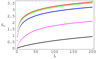
Figure 7: Entropy of the reduced density matrix for $L$ spins in the isotropic XX model, $\gamma=0$, with different external magnetic field $\lambda$. The maximum entropy is reached when there is no applied external field. The entropy decreases while the magnetic field increases until $\lambda=1$ when the system reaches the ferromagnetic limit and the ground state is a product state in the spin basis.

It is easy to extend our computation to other critical and non-critical points in the parameter space for the XY system. Fig. (8) shows the scaling of entanglement as we scan $\gamma$. Note again the logarithmic scaling of the entropy although its coefficient is now 1/6 instead of 1/3. The constant correction to the logarithmic scaling is such that

$$S^{XY}_{L}=\frac{1}{6}\log_{2}L+a(\gamma),$$ (86)

so that

$$\lim_{L\rightarrow\infty}\left[S_{L}(\gamma=1)-S_{L}(\gamma)\right]=-\frac{1}{6}\log_{2}\gamma\ .$$ (87)

Figure 8: Difference of the entropy $\lim_{L\rightarrow\infty}\left[S_{L}(\gamma=1)-S_{L}(\gamma)\right]$ for different values of the anisotropy $\gamma$. For every $\gamma$ the model is critical and the entropy scales as ${1/6}\log_{2}L+a(\gamma)$, where the $L$-independent function $a(\gamma)$ is perfectly fitted by $-\frac{1}{6}\log_{2}\gamma$.

When $\gamma=1$ the system is described by the Ising model. The entropy behavior in this limit can be viewed in the Fig. (9). When the magnetic field is turned to $\lambda=1$ the entropy reproduces the scaling law

$$S^{Ising}_{L}=\frac{1}{6}\log_{2}L+a\qquad\gamma=1,\,\lambda=1.$$ (88)

In this model, the least square fit of the logarithmic behavior gives a standard error of $4\,10^{-9}$. For the Ising model with no external field, the ground state that minimizes the total energy is the Néel state, a macroscopic GHZ state, for which the entropy is always equal to one.

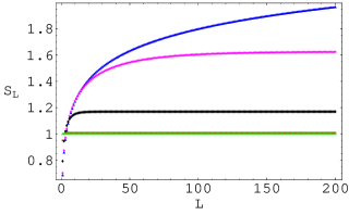
Figure 9: Entropy for the reduced density matrix to $L$ spins of the Ising model, $\gamma=1$, with different values of the external magnetic field, $\lambda\in\{0,1\}$. The maximum entropy is reached at the critical point when the applied field is one. Other values of the magnetic field lead to saturation of the entropy. For a magnetic field $\lambda=0$ the ground state of the system is in the Néel state or GHZ state.

IV Heisenberg model

IV.1 The XXZ Hamiltonian

The XXZ model consists of a chain of $N$ spins with nearest neighbor interactions and an external magnetic field, as given by the Hamiltonian

$$H_{XXZ}=\sum_{l}\left(\frac{1}{2}[\sigma^{x}_{l}\sigma^{x}_{l+1}+\sigma^{y}_{l}\sigma^{y}_{l+1}+\Delta\sigma^{z}_{l}\sigma^{z}_{l+1}]+\lambda\sigma^{z}_{l}\right).$$ (89)

As in the previous section, $l$ labels the $N$ spins and $\sigma_{l}^{\mu}$ ($\mu=x,y,z$) are the Pauli matrices, Eqs. (23)-(24). Parameter $\Delta$ evaluates the anisotropy, in the $z$ direction, of the antiferromagnetic Heisenberg interaction, whereas $\lambda$ is the strength of a magnetic field applied in the $z$ direction.

The XXZ model includes as special cases two other well-known spin models. The XXX model corresponds to a fully isotropic interaction, $\Delta=1$,

$$H_{XXX}=\sum_{l}\left(\frac{1}{2}[\sigma^{x}_{l}\sigma^{x}_{l+1}+\sigma^{y}_{l}\sigma^{y}_{l+1}+\sigma^{z}_{l}\sigma^{z}_{l+1}]+\lambda\sigma^{z}_{l}\right).$$ (90)

Also, when the interaction in restricted to the plane $xy$ in spin space, $\Delta=0$, we recover the XX model of Eq. (26).

These Hamiltonians are commonly used to model the physics of certain spin chains, but also to describe other quantum systems. For instance, the XXX Hamiltonian without magnetic field can be obtained in a particular limit of the fermion Hubbard model,

$$H=\sum_{l\tau}\left(\epsilon n_{l\tau}+t(\hat{h}^{\dagger}_{l\tau}\hat{h}_{l+1\tau}+\hat{h}^{\dagger}_{l+1\tau}\hat{h}_{l\tau})\right)+\sum_{l}Un_{l\uparrow}n_{l\downarrow},$$ (91)

where $\hat{h}$ are fermionic annihilation operators,

$$\{\hat{h}_{l\tau},\hat{h}_{m\nu}^{\dagger}\}=\delta_{lm}\delta_{\tau\nu},$$ (92)

$n_{l\tau}=\hat{h}_{l\tau}^{\dagger}\hat{h}_{l\tau}$ are fermion number operator and $l$ labels one of $N$ sites of a chain while $\nu$ denotes one of two spin orientations, $\uparrow$ or $\downarrow$. The fermion Hubbard Hamiltonian (see chapter 10 of sach99 ) was originally introduced to describe the motion of electrons in transition metals, and consists of spin-1/2 fermionic particles moving along the $N$ sites. Parameter $\epsilon$ is the energy cost of having one fermion, $t$ is the tunneling parameter and $U$ quantifies the interaction between two fermions at the same site. Notice that the total number of fermions $n=\sum_{l\tau}n_{l\tau}$ is a constant of motion. Then, when restricted to a subspace with a given value of $n$, the first term in the Hamiltonian is proportional to the identity and can be omitted. Let us consider the case when the total number of fermions is $N$, that is, the same as the number of sites. In the limit $U\gg t$, two fermions are not energetically allowed to be on the same site, and we have one fermion per site. In this limit, and with the identification

$$\sigma_{l}^{x} = \hat{h}_{l\uparrow}^{\dagger}\hat{h}_{l\downarrow}+\hat{h}_{l\uparrow}^{\dagger}\hat{h}_{l\downarrow},$$ (93)

$$\sigma_{l}^{y} = -i(\hat{h}_{l\uparrow}^{\dagger}\hat{h}_{l\downarrow}-\hat{h}_{l\uparrow}^{\dagger}\hat{h}_{l\downarrow}),$$ (94)

$$\sigma_{l}^{z} = \hat{h}_{l\uparrow}^{\dagger}\hat{h}_{l\uparrow}-\hat{h}_{l\downarrow}^{\dagger}\hat{h}_{l\downarrow},$$ (95)

the Hubbard model can be recast (using perturbation theory) into the isotropic Heisenberg model without magnetic field,

$$H=J\sum_{l}\vec{\sigma}_{l}\cdot\vec{\sigma}_{l+1},$$ (96)

where $J=4\frac{t^{2}}{U}$. Metal-insulator transitions, superconductive systems or magnetic properties can be explained with this Hamiltonian.

Quantum phase transitions are identified with points of non-analyticity in the ground state energy of the spin chain. This non-analyticity may appear in the limit of a large chain or, as in the present case, may be due to level crossing. Notice that we can decompose $H_{XXZ}$, Eq. (89), in terms of three commuting parts,

$$H_{XXZ}=H_{1}+\Delta H_{2}+\lambda H_{3}.$$ (97)

As we change $\Delta$ or $\lambda$, an excited state may see its energy decreased enough as to become the ground state. At one such point, the ground state energy $E(\Delta,\lambda)$ will not be analytical. Thus, in this model quantum phase transitions occurs for finite chains.

IV.2 Bethe Ansatz for the Heisenberg model

Several properties make the Heisenberg Hamiltonian with periodic boundary conditions completely integrable. Two symmetries are essential to get the model solution and are used in the Bethe Ansatz (BA) bet01 . Rotational symmetry about the $z$-axis in spin space implies that the $z$-component of the total spin $S^{z}_{T}$,

$$S^{z}_{T}=\frac{1}{2}\sum_{l}\sigma_{l}^{z},$$ (98)

is conserved. Sorting the basis vectors according to the quantum number $S^{z}_{T}=N/2-r$, where $N$ is the number of sites in the chain and $r$ the number of spins down, is all that is required to block diagonalize the Hamiltonian. The second symmetry is the invariance of $H$ with respect to discrete translations by any number of lattice spacings. To reconstruct the whole spectrum of the Heisenberg model, Bethe’s idea is to start with the ferromagnetic state $|F\rangle$,

$$\mbox{$|F\rangle$}=\mbox{$|\uparrow\uparrow\cdots\uparrow\rangle$},$$ (99)

whose spin angular momentum, $\frac{N}{2}$, is maximum, and to get a translationally invariant eigenstate of the Hamiltonian with one unit less of spin angular momentum. The rest of the spectrum of the Heisenberg model is obtained by iterating this process.

Here, we shall use the BA to get a numerical but exact solution of a finite spin chain. Finite size effects are present but can be controlled by comparing different sizes. Scaling of entanglement is thus approached asymptotically as the size grows. For a fixed value of $S^{z}_{T}=N/2-r$, eigenstates are of the form

$$|\Psi\rangle=\sum_{1\leq n_{1}<...<n_{r}\leq N}a(n_{1},...,n_{r})|n_{1},...,n_{r}\rangle,$$ (100)

where $n_{1},\cdots,n_{r}$ list the position of the $r$ spin that are down, and $a(n_{1},\cdots,n_{r})$ fulfills

$$a(n_{1},...,n_{r})=\sum_{\mathcal{P}\in\mathcal{S}_{r}}\exp\left(\rm{i}\sum_{j=1}^{r}k_{\mathcal{P}j}n_{j}+\frac{\rm{i}}{2}\sum_{i\leq j}\theta_{\mathcal{P}i,\mathcal{P}j}\right).$$ (101)

Here $\mathcal{P}\in\mathcal{S}_{r}$ denotes one of the $r!$ permutations of $\{1,...,r\}$ and $k_{i}$ and $\theta_{i,j}$ with $(i,j)\in\{1,...,r\}$ are the parameters to be determined.

Three general conditions hold for these parameters orb01 :

$$\theta_{i,j} = -\theta_{j,i}\leavevmode\nobreak\ \leavevmode\nobreak\ \leavevmode\nobreak\ \leavevmode\nobreak\ \leavevmode\nobreak\ \leavevmode\nobreak\ \leavevmode\nobreak\ \leavevmode\nobreak\ \leavevmode\nobreak\ \leavevmode\nobreak\ \forall\{i,j\},$$

$$\cot\frac{\theta_{i,j}}{2} = \frac{\Delta\sin\frac{k_{i}-k_{j}}{2}}{\cos\frac{k_{i}+k_{j}}{2}+\Delta\cos\frac{k_{i}-k_{j}}{2}}\hskip 12.91663pt(i,j)\in\{1,...,r\},$$

$$Nk_{i} = 2\pi\lambda_{i}+\sum_{j\neq i}\theta_{i,j}\leavevmode\nobreak\ \leavevmode\nobreak\ \leavevmode\nobreak\ \leavevmode\nobreak\ \leavevmode\nobreak\ \leavevmode\nobreak\ \leavevmode\nobreak\ \leavevmode\nobreak\ \leavevmode\nobreak\ \leavevmode\nobreak\ i\in\{1,...,r\},$$ (102)

where the integers $\lambda_{i}$ are called Bethe quantum numbers. The states are completely determined by the Bethe quantum numbers and Eqs. (100)-(IV.2).

It is known yan01 that the set $\{\lambda_{i}\}$ with the lowest energy for each ${S}^{z}_{T}=N/2-r$ satisfies:

$$\lambda_{i}={S}^{z}_{T}-1+2i=\frac{N}{2}-r-1+2i\hskip 12.91663pti\in\{1,...,r\}.$$ (103)

The expression for the ground state energy reads

$$E-E_{F}=-J\sum_{i=1}^{r}(\Delta-\cos k_{i})+\lambda S^{z}_{T},\hskip 12.91663ptE_{F}=\frac{JN\Delta}{4}.$$ (104)

We have found convenient to solve the previous system of non-linear equations using a minimization code for absolute errors based on genetic algorithms, although many other numerical techniques could have been used. Precision can be controlled by setting a maximum bound in the numerical error in the parameters $\theta$’s and $k$’s to $10^{-5}$. This small error has proven enough to detect the scaling of entropy. The systems that we study have an even number of sites $N$, so the eigenvalue of the $S^{z}_{T}$ operator in the ferromagnetic system is the integer $N/2$.

IV.3 Entropy of a block of spins

The fact that the BA is used to compute numerically the eigenvalues of the reduced density matrix of blocks of spins limits the size of the system that can be studied. The results we obtain are thus less precise than those for the XY model although scaling laws can be inferred with confidence. As a first step, we concentrate on the effect of the finite size system for the entropy results. More precisely, we analyze the isotropic model without magnetic field in a chain of $N=\{8,10,12,14,16,18\}$ sites. The results are plotted in Fig. (10). Finite size effects bend down the entropy when the size of the block approaches half of the chain. Smaller blocks are less sensitive to the finite size and show good scaling. The numerical results indicate that the entropy behavior converges to a logarithmic scaling when as the size of the system increases. This asymptotic behavior corresponds to

$$S_{L}\sim\frac{1}{3}\log_{2}L\ .$$ (105)

As we shall discuss in the next two sections, this entropy scaling falls into the universality class of a free boson.

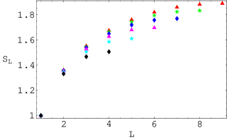
Figure 10: Dependence of the entropy $S_{L}$ on the finite size of the chain in the isotropic Heisenberg model without magnetic field. In the plot, triangles, stars, diamonds, triangles, stars and diamonds correspond to 18, 16, 14, 12, 10, and 8 spins chains, respectively. All curbs coincide with the upper one for low block sizes $L$, but disagree as $L$ gets closer to $N/2$ due to a finite-size saturation effect.

IV.3.1 Isotropic model in a magnetic field

We first analyze the XXX model with a magnetic field, Eq. (90). We can now use the BA to compute the eigenstates of the Hamiltonian in the critical interval: $\lambda\in[0,2)$  bon01 . For values of $|\lambda|$ greater or equal to 2, every spin in the system is pointing in the magnetic field direction and the state is a product of $S^{z}_{i}$ eigenstates. Entanglement has disappeared.

As implicit in the BA, the ground state has a well defined magnetization, $S^{z}_{T}$. This quantity changes every time the tuning of the magnetic field implies a new level-crossing. The relation between the magnetization, $S^{z}_{T}$, and the ratio $\lambda$ between the magnetic field $\lambda$ and the coupling constant $J$ is well defined and can be easily obtained from the spectrum of the model.

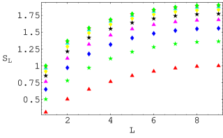
Figure 11: Entropy $S_{L}$ in a ring of $N=18$ spins, for blocks of size up to $L=N/2=9$ spins. The curbs correspond to the values of the magnetic field, $\lambda\in\{0,0.24,0.68,1.05,1.35,1.59,1.77,1.89,1.97\}$, for which there is level crossing. For a given $L$, the entropy remains constant in the interval between level crossing, but every time the coupling is at one of the latter points the entropy value changes. The maximum in the entropy is obtained for the antiferromagnetic system without magnetic field, while it goes to zero as $\lambda$ approaches 2.

The Heisenberg model has two limiting behaviors. On the one hand, for $\lambda=0$ the ground state is antiferromagnetic, with a null angular momentum eigenvalue. On the other hand, for $\lambda\geq 2$, the ground state of the system corresponds to the ferromagnetic state $|F\rangle$. Figs. (11) and (12) illustrate how the entropy of a finite spin ring changes when $\lambda$ varies in the interval $[0,2]$. Fig. (11) shows the way the entropy decreases as $\lambda$ increases, obtaining the zero value when $\lambda\to 2$ where the ground state turns into a product state. The plotted values of $\lambda$ are those for which the ground state has a level crossing for a ring with $N=18$ sites. The ground state, and therefore also its entropy, remain constant in the interval between level crossings. Fig. (12) plots the way the entropy increases logarithmically when $\lambda$ decreases, keeping the number of traced spins fixed.

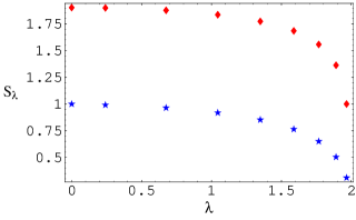
Figure 12: Entropy $S_{L}$ in a ring of $N=18$ spins, for different values of the magnetic field $\lambda$. Stars correspond to the reduced density matrix of one spin, $S_{L=1}$, and diamonds to the reduced density matrix for half ring, $S_{L=N/2=9}$.

IV.3.2 Anisotropic model

Let us now analyze the behavior of entanglement as a function of the anisotropy $\Delta$ in a Heisenberg chain without magnetic field, that is $H_{XXZ}$ with $\lambda=0$ in Eq. (89).

In this case, the critical interval aff01 corresponds to $\Delta\in[-1,1]$. For $\Delta=1$ we recover the isotropic antiferromagnetic model, $H_{XXX}$. In the case $\Delta=-1$ the Hamiltonian can be transformed into the isotropic ferromagnetic Hamiltonian,

$$H=-\sum_{l}\vec{\sigma}_{l}\cdot\vec{\sigma}_{l+1},$$ (106)

by further rotating each second spin by 180 degrees in the z direction. Notice that entanglement remains invariant under this transformation. This argument shows that entanglement is a robust magnitude and depends on fewer details of the system than e.g. its magnetization.

The anisotropy is a marginal deformation in the interval $\Delta\in[-1,1]$, in that for any such value of $\Delta$ the system has the same large scale behavior. Instead, for other values of $\Delta$ a gap appears in the spectrum, giving raise to a new length scale. A finite correlation length in the system takes over and all correlations decay exponentially. Fig. (13) shows that in this case the entropy $S_{L}$ gets saturated as a function of $L$.

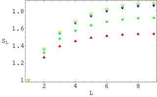
Figure 13: Entropy $S_{L}$ in a ring of $N=18$ spins and for different values of the anisotropy $\Delta$. The critical interval is for $\Delta\in[-1,1]$, and leads to the upper, superposed curbs. The points out of the critical interval are diamonds with $\Delta=1.5$, stars with $\Delta=2.0$ and triangles with $\Delta=2.5$. Thus, as we change the anisotropy $\Delta$ away from the critical interval, the entropy gets saturated by a value that decreases with $\Delta$.

V Critical versus non-critical entanglement

We now turn to analyze the results of the calculations described in the previous two sections.

The big picture emerging from these calculations is that there is a clear distinction between the entanglement in a non-critical chain and that in a critical chain, as measured by the entropy $S_{L}$ of the reduced density matrix $\rho_{L}$ for $L$ contiguous spins, see Figs. (7) and (9). For all non-critical models, $S_{L}$ reaches a saturation value $S^{*}$ as $L$ increases, whereas for critical chains $S_{L}$ grows unboundedly with $L$.

V.1 Non-critical spin chains

Recall that in the non-critical regime, a spin chain is characterized by a gap between the energy of the ground state and that of the first excited state. Relatedly, correlations between increasingly distant spins decay exponentially,

$$\mbox{$\langle\sigma^{a}_{l}\sigma^{b}_{l+L}\rangle$}-\mbox{$\langle\sigma^{a}_{l}\rangle$}\mbox{$\langle\sigma^{b}_{l+L}\rangle$}\sim\exp(-L/\xi),$$ (107)

where $\xi$ is the correlation length (we take the distance between nearest spins as unit of distance). For non-critical chains, we find that the entropy $S_{L}$, a growing function with the block size $L$, is upper-bounded by a saturation value $S^{*}$. This value depends on the parameters specifying the spin chain, and becomes larger as the chain gets closer to a critical point or critical phase. For any fixed value of the parameters specifying the spin model, $S_{L}$ approaches the saturation value $S^{*}$ for block sizes $L$ of the order of the correlation length $\xi$. We can conclude, therefore, that the entanglement between a block and the rest of an infinite spin chain has a fixed value for blocks larger than the correlation length $\xi$.

Recall from Eq. (15) that $S_{L}$ could in principle grow as much as $L$. This means that, for large block size $L$, the entanglement of a block is negligible when compared to its maximal possible value,

$$\lim_{L\rightarrow\infty}\frac{S^{*}}{L}=0.$$ (108)

Thus, the ground state $|\Psi_{g}\rangle$ entangles all the spins in the chain, either directly or through intermediate spins, but the system does only contain a very small amount of entanglement at any scale.

The above calculations can be used not only to obtain $S_{L}$, but also to determine the whole spectrum Sp$(\rho_{L})$ of decreasingly ordered eigenvalues $\{p_{L}^{i}\}$ of the reduced density matrix $\rho_{L}$ for the block (see section VI.3). For any $L$, this spectrum contains only a very small number of relevant eigenvalues, together with many small, rapidly decaying eigenvalues with an insignificant overall weight. Thus, in spite of a exponential growth of the rank of $\rho_{L}$ with $L$, the effective rank $\raisebox{1.29167pt}{$\chi$}_{L}^{\rm\epsilon}$ (recall section II.3) also gets saturated, with the saturation value $\raisebox{1.29167pt}{$\chi$}^{\rm\epsilon}$ being reached when $L$ is of the order $\xi$.

From the point of view of numerical calculations, the saturation of $\raisebox{1.29167pt}{$\chi$}_{L}^{\epsilon}$ can be used to interpret the extraordinary success of the DMRG in non-critical spin chains and other one-dimensional systems. Only a fixed, small number of eigenvectors of $\rho_{L}$ must be retained in order to capture the relevant degrees of freedom as $L$ increases RO99 . Similarly, a bounded effective rank $\raisebox{1.29167pt}{$\chi$}_{L}^{\epsilon}$ as a function of $L$ indicates that non-critical spin chains can be efficiently simulated using the techniques introduced in gvprep .

V.2 Critical chains

The energy spectrum of a critical spin chain is gapless and the two-spin correlation function is characterized by a power scaling law,

$$\mbox{$\langle\sigma^{a}_{l}\sigma^{b}_{l+L}\rangle$}-\mbox{$\langle\sigma^{a}_{l}\rangle$}\mbox{$\langle\sigma^{b}_{l+L}\rangle$}\sim L^{-q},$$ (109)

where $q>0$ (there are cases where marginal deformations lead to logarithmic corrections to the power law). This scaling law implies an infinite correlation length $\xi$. For critical spin chains we have obtained that $S_{L}$ grows unboundedly as a function of $L$. In particular, in all the cases we have analyzed the growth of $S_{L}$ is asymptotically given by

$$S_{L}\sim k\log_{2}L,$$ (110)

where $k$ is either $1/3$ or $1/6$ depending on the parameters of the critical chain. Thus, for critical spin chains the entanglement between a block of spins and the rest of a chain grows unboundedly with the size $L$ of the block, in sharp contrast with the non-critical case. In the next section we will elaborate on the particular shape (110) of $S_{L}$ for critical chains.

Given fixed computer memory and execution time, the DMRG works with significantly smaller accuracy for critical spin chains than for non-critical ones. This result can now be qualitatively interpreted in terms of the arbitrarily large entanglement that links a spin block to the rest of the chain as $L$ grows. Indeed, a larger value of $S_{L}$ implies that more eigenstates of $\rho_{L}$ must be retained in order for the DMRG to achieve a similar accuracy as when $S_{L}$ is small (recall Eq. (21)).

We notice that even if $S_{L}$ for critical chains grows unboundedly with $L$, we again have that its value is much smaller than the upper bound (15), $S_{L}/L$ becoming negligible for large $L$. Therefore, even if entanglement is the responsible for the appearance of long-range correlations at a critical point, we find that the amount of entanglement in the ground state of a spin chain is surprisingly small compared to its maximal possible value.

Finally, in section VI it will be argued that in $d\geq 2$ dimensions, the entanglement between a $d$-dimensional block of $L^{d}$ spins and the rest of a critical spin lattice grows as $L^{d-1}$. The same scaling is expected to apply to non-critical spin lattices. This implies that $\raisebox{1.29167pt}{$\chi$}_{L}^{\rm\epsilon}$ grows exponentially with the size of the block, explaining the systematic breakdown of the DMRG in quantum spin systems in more than one dimension.

VI Scaling of entanglement and conformal field theory

The set of results found in the previous sections exemplify the connection between entanglement and quantum field theory concepts. The bridge between quantum information and quantum field theory can be further explored and exploited in both directions. In this sense, we shall translate results from black hole entropy and effective actions on gravitational backgrounds to the language of quantum information. Working in the opposite direction, quantum information natural measures of order based on majorization theory seem to find their way into renormalization group irreversibility. The cross-fertilization of these ideas requires a change of language and quite a lot of background on quantum field theory that we cannot cover here in a self-contained or satisfactory way. Nevertheless, we will very briefly review some concepts in conformal field theory and c-theorem necessary to state their spinoff in quantum information theory.

VI.1 Entropy and conformal field theory

The study of entropy in systems with an infinite number of degrees of freedom has received quite some attention in the context of quantum field theory and black hole physics. Historically, the thermodynamics of a black hole lead to the Bekenstein-Hawking entropy (see for instance Be94 . This entropy is associated to the counting of microscopic degrees of freedom inside the horizon and scales as the area of the black hole. Some authors suggested that the origin of this entropy might be rooted in the loss of information forced upon an external observer by the existence of a horizon. Although this point of view is no longer pursued, its analysis comes naturally due to the combination of quantum mechanics and general relativity which underlies the holographic principle. The field theoretical definition of entropy faces the traditional problem of renormalization in quantum field theory and receives the name of fine-grained entropy as well as geometric entropy.

Three computations of genuine quantum field theory entropy are worth recalling. First, Srednicki Sr93 considered a properly regularized massless bosonic field theory in a universe which is divided by an imaginary sphere of radius $R$ into its inside and outside parts. He then numerically constructed the density matrix of the reduced outside system and found that its entropy scaled with an area law in 3+1 dimensions. For 1+1 dimensions, the scaling behavior of the entropy was found to be logarithmic. Second, Callan and Wilczek Ca94 put forward the concept of geometric entropy in 1+1 dimensions. There, the power of conformal symmetry was used at full steam in order to compute the entropy of a conformal field theory when reduced to a finite geometry. We shall come back to this result shortly. Finally, the third relevant computation was carried out by Fiola, Preskill, Strominger and Trivedi Fi94 who mapped a regularized field theory in 1+1 dimension to the Rindler coordinates and recovered the logarithmic behavior of the microscopic entropy. All these computations needed an explicit ultraviolet regulator since quantum field theory contains infinitely many degrees of freedom. Note that in our case spin chains come equipped with the intrinsic ultraviolet cutoff of the lattice spacing.

Although more restrictive in scope, the computation of the geometric entropy of a 1+1 dimensional field theory brings the advantage that the result is casted in terms of the parameters that classify conformal field theories. More concretely, the result found by Holzhey, Larsen and Wilczek HoLaWi reads

$$S_{L}=\frac{c+\bar{c}}{6}\log_{2}L$$ (111)

where $c$ and $\bar{c}$ are the so called central charges for the holomorphic and antiholomorphic sectors of the conformal field theory.

Let us briefly recall that conformal field theories cft are classified by the representations of the conformal group in 1+1 dimensions. The operators of the theory fall into a structure of highest weight operators and its descendants. Each highest weight operator carries some specific scaling dimensions which dictates those of its descendants. The operators close an algebra implemented into the operator product expansion. One operator is particularly important: the energy-momentum tensor $T_{\mu\nu}$. It is convenient to introduce holomorphic and antiholomorphic indices defined by the combinations $T=T_{zz}$ and $\bar{T}=T_{\bar{z}\bar{z}}$ where $z=x^{0}+ix^{1}$ and $\bar{z}=x^{0}-ix^{1}$. Denoting by $|0\rangle$ the vacuum state, the central charge of a conformal field theory is associated to the coefficient of the correlator

$$\langle 0|T(z)T(0)|0\rangle=\frac{c}{2z^{4}}$$ (112)

and the analogous result for $\bar{c}$ in terms of the correlator $\langle 0|\bar{T}(z)\bar{T}(0)|0\rangle$. A conformal field theory is characterized by its central charge, the scaling dimensions and the coefficients of the operator product expansion. Furthermore, unitary theories with $c<1$ only exist for discrete values of $c$ and are called minimal models. The lowest lying theory corresponds to $c=\frac{1}{2}$ and represents the universality class of a free fermion.

The central charge plays many roles in a conformal field theory. It was introduced above as the coefficient of a correlator of energy-momentum tensors, which means that it is an observable. The central charge also characterizes the response of a theory to a modification of the background metric where it is defined. Specifically, the scale anomaly associated to the lack of scale invariance produced by a non-trivial background metric is

$$\langle 0|T^{\mu}_{\mu}|0\rangle=-\frac{c}{12}R$$ (113)

where $R$ is the curvature of the background metric. This anomaly can also be seen as the emergence of a non-local effective action when the field theory modes are integrated in a curved background.

The results we have found in our analysis match perfectly the geometric entropy computation. In the case of the XX and Heisenberg critical spin chains the central charge is $c=\bar{c}=1$ and the model falls into the free boson universality class. The critical Ising model corresponds to a free fermion, thus $c=\bar{c}=\frac{1}{2}$. The central charge of the theory is seen to play the role of a measure of entanglement. The vacuum of a theory of free bosons is more entangled than the one corresponding to a theory of free fermions. Scaling of entanglement is just another manifestation of the ubiquitous organizing principle orchestrated by conformal symmetry. The amount of surprise (or entropy) obtained when in a given theory a new degree of freedom (a new spin in the block) is added must follow scaling as dictated by the representation of conformal symmetry corresponding to that theory. Because the entropy of the reduced density matrix of the ground state is not attached to any particular operator, it is natural that the central charge is the parameter in control of this measure of entanglement.

Due to the relation between entanglement and the central charge a number of further connections appear. The central charge quantifies quantum correlations as well as e.g. the trace anomaly. A plausible interpretation can now be given in terms of entanglement. The more quantum correlated the vacuum is, the stronger the breaking of conformal symmetry appears when a curved background is present. More relevant is how the theorem on irreversibility of renormalization group flows translates to entanglement in a way that will be discussed shortly.

VI.2 Entanglement in higher dimensional systems

Entanglement in spin chains obeys logarithmic scaling. This result was seen to emerge from conformal symmetry. It is then possible to apply similar arguments in higher dimensions and complete them with standard arguments based on the Schmidt decomposition.

Let us consider a $d+1$ field dimensional theory at its critical point. Its ground state is a pure state. Following Srednicki Sr93 , one could now consider the reduced system on e.g. a hypersphere $S^{d-1}$ of radius $R$. The division into the interior $A$ and the exterior $B$ of this imaginary hypersphere can be used to write the ground state using the Schmidt decomposition in terms of pure states $|\xi_{i}\rangle,|\phi_{i}\rangle$ associated to each region

$$\mbox{$|0\rangle$}=\sum_{i}\sqrt{p_{i}}|\xi_{i}\rangle_{A}|\phi_{i}\rangle_{B}\ ,$$ (114)

where $p_{i}$ are positive numbers and the sum ranges up to the minimum of the dimensions of the Hilbert spaces for A and B. The standard argument follows that both reduced density matrices share the same eigenvalues $p_{i}$ and, thus, the same entropy. Yet, both systems only share the hypersurface separating them, so that the leading term of the entropy as any infrared cutoff is sent to infinity and the ultraviolet cutoff $x_{uv}$ is sent to zero must scale as its “area”

$$S_{R}=c_{1}\leavevmode\nobreak\ \left(\frac{L}{x_{uv}}\right)^{d-1}$$ (115)

where $c_{1}$ is a known coefficient related to anomalies that we shall discuss later. This leading scaling law for $x_{uv}\to 0$ also holds for massive particles as checked by explicit calculations in free massive theories kabat . The “area” law associated with the hypersurface is understood as an effect coming from the loss of coherence between the points at each side of the boundary separating the interior and exterior parts of the universe. It is then natural to expect that microscopic condensed matter systems will follow the same law.

At variance with spin chains, the ultraviolet cutoff $x_{uv}$ gets now mixed with the global coefficient $c_{1}$ and it is unclear how to extract observable information from the latter. It has been shown that $c_{1}$ corresponds to the coefficient of the linear term in the curvature in the effective action of a field theory in a non-trivial gravitational background kabat . Then, $c_{1}$ equals 1/6 for scalar particles and 1/12 $2^{[d/2]}$ for Dirac fermions. More precisely, every fermionic component contributes to $c_{1}$ as half a boson. In 1+1 dimensions, we worked with spinless fermions, thus the relative factor of 2 between 1/6 for the critical Ising model and 1/3 for the XX and Heisenberg critical chains. In dimension 3+1, the entropy of a system of a free Dirac fermion will carry twice more entropy than a free boson since the Dirac fermion is made of four components.

Entanglement is thus also connected through Eq. (115) to the effective action of quantum field theories on gravitational backgrounds. It is a remarkable fact that in $1+1$ dimensions the effective action has a unique non-local form proportional to the central charge $c$. When this non-local action is expanded in powers of the curvature, all terms carry the dependence in $c$. It follows that the trace anomaly, which is a derivative of this effective action with respect to the metric, is also proportional to the central charge. This is no longer true in higher dimensions. The effective action of a quantum field theory defined on a gravitational background develops infinitely many apparently unrelated structures. The entropy of entanglement seems to be related to $c_{1}$ kabat , the coefficient of the linear term in the curvature $R$ (called $a_{1}$ in birrel ). On the other hand, other contributions to the trace anomaly giving rise to the Euler density and to non-trivial two-point energy-momentum tensor correlators are related to the structures that come quadratic with the curvature. All the coefficients in the effective action seem to quantify different aspects of entanglement.

A remarkable result concerning the saturation of entanglement in non-critical systems can also be translated from quantum field theory to spin chains. It has been proven kabat that the leading order result when the ultraviolet cutoff is sent to infinity, Eq. (115) is not modified by adding a mass to the scalar field. The leading behavior of entanglement is not affected by going away from conformal symmetry because the contribution to the entropy comes from the entanglement between points near each side of the boundary (see also Ga01 ). The scaling law in terms of the hypersurface separating them is respected although a finite correlation length is present. Moreover, the subleading corrections to the “area” law are known when $x_{uv}\ll\frac{1}{m}\ll x_{ir}$, $x_{ir}$ being an infrared cutoff which defines a separation of space in two regions in analogy to our previous $R$,

$$S_{m}-S_{m=0}=\begin{cases}-\frac{x_{ir}m}{24\pi}&d=2+1\cr\frac{x_{ir}^{2}m^{2}}{96\pi^{2}}\ln{mx_{uv}}&d=3+1\cr\end{cases}$$ (116)

where the subindex $m$ labels the massive theory. The case $d=1+1$ corresponds to the universality class we have been discussing in systems of spin chains and yields the following result kabat

$$S=-\frac{1}{6}\ln mx_{uv}\qquad x_{uv}\ll\frac{1}{m}\ll x_{ir}\ .$$ (117)

This latter result is indeed observed in our computation (and will be presented more extensively in some other publication). For instance, the external magnetic field deformation of the Ising model $(\gamma=1,\lambda\neq 1)$, Fig. (9), corresponds to an effective mass $m\sim|1-\lambda|$.

The lack of saturation of entanglement in massive theories have clear implications for the application of DMRG techniques as well as other modifications of the Wilsonian block-spin idea for condensed matter systems. Entanglement always diverges (even off criticality) in more than 1+1 dimensions and limits the success of such an approach. It seems conceptually preferable to construct projections of the exact renormalization group based in momentum space as the local potential approximation. This method has proven quite powerful in scalar theories erg where it provides good approximations to critical exponents in any number of dimensions and can even detect triviality.

VI.3 Majorization and entanglement

Let us return to quantum spin chains where entanglement pervades the system at conformal points. The absence of a mass scale makes quantum correlations extend to long distances. Consequently, the vacuum structure must describe this fact and the entropy shows scaling as discussed above. It is arguable that the entropy of the vacuum in the reduced system is just one out of many possible measures of entanglement. Then, other yet unexplored measures of entanglement may bring further information about the structure of the vacuum.

In order to investigate this issue, we can further exploit our computations due to the fact that we have explicit results for the density matrix of the ground state in the Ising and XX models. The $2^{L}$ eigenvalues of $\rho_{L}$ correspond to the product of the $2$ eigenvalues $(1\pm\nu_{m})/2$ of $L$ fermionic modes, Eq. (81),

$$\lambda_{x_{1}x_{2}\cdots x_{L}}=\prod_{m=0}^{L-1}\frac{1+(-1)^{x_{m}}\nu_{m}}{2},\leavevmode\nobreak\ \leavevmode\nobreak\ \leavevmode\nobreak\ x_{m}=0,1\leavevmode\nobreak\ \forall m.$$ (118)

It is convenient to first visualize the typical shape of the eigenvalues $(1\pm\nu_{m})/2$ of the fermionic modes and observe that most of the $\rho_{L}$ eigenvalues are almost zero or one and only a small set will take intermediate values, bringing the main contribution to the entropy. Each mode tends to remember its pure state origin.

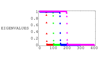
Figure 14: Plot of the eigenvalues $\frac{1\pm\nu_{m}}{2}$ of the fermionic modes, Eq. (81), for the Ising model, Eq. (25), and $L=\{50$ (triangles), $100$ (stars), $150$ (diamonds), $200$ (triangles)$\}$. As $L$ increases new modes are populated.

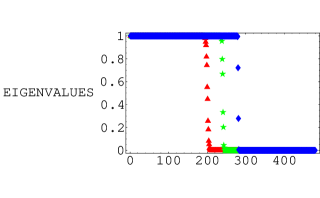
Figure 15: Plot of the eigenvalues $\frac{1\pm\nu_{m}}{2}$ of the fermionic modes, Eq. (81), for the XX model as a function of the magnetic field $\lambda$, Eq. (26), taking $L=200$ spins from an infinite ring. Triangles display the eigenvalues for $\lambda=0.5$, stars for $\lambda=0.999$ and diamonds the eigenvalues for $\lambda=0.99999$. When $\lambda$ approaches 1, the ground state becomes a product state and the modes take only the value one or zero. The three plots should overlap each other, but we have artificially shifted each plot 40 points respect to the previous one.

The eigenvalues of $\rho_{L}$ form a probability distribution. It is numerically easy verified that at conformal points

$$\rho_{L+2}\prec\rho_{L}\ ,$$ (119)

that is, the probability distributions associated to the density matrices obey a majorization relation. Due to the spin structure of the problem the majorization takes place at two-spin steps. We have verified that a similar result about majorization holds for the quantum Ising model at its critical point.

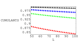
Figure 16: Plot of the cumulants of the 8 (triangles), 16 (stars), 32 (diamonds) and 64 (triangles) larger probabilities associated to the ground state $\rho_{L}$ as a function of $L$ in steps of 2 in the XX model without magnetic field.

The increase of amount of surprise quantified by the entropy is rooted in a deeper sense of ordering in the vacuum. The ground state $\rho_{L}$ becomes more and more disordered as dictated by a majorization arrow. Note that this implies and increasing number of relations between the eigenvalues of $\rho_{L}$ as $L$ goes to infinity. The vacuum in a field theory is far more ordered than what the scaling of entropy hints at, in the sense that majorization provides a more strict definition of order than entropy.

In order to establish the role of majorization and its relation to conformal symmetry, further work is necessary. In particular, marginal deformations need to be analyzed carefully. Later on we shall argue that a different type of majorization seems to hold along renormalization group flows. In that case, $L$ is kept fixed but the parameters of the hamiltonian change as dictated by renormalization group transformations.

VI.4 Irreversibility of entanglement and the c-theorem

Given the relation between entanglement and conformal symmetry, some powerful quantum field theory results can be borrowed and translated to quantum information parlance. It is of particular relevance the so called Zamolodchikov’s c-theorem zam86 that establishes that the central charge of a unitary 1+1 dimensional theory always decreases along renormalization group trajectories. The existence of a c-theorem in more than 1+1 dimensions has been a subject of a lot of effort Ca88 ; cfl91 ; clv92 ; osbo ; anse and a proof has been proposed in fl98 . Zamolodchikov’s theorem in 1+1 dimensions can be proven using the spectral densities following Ref. cfl91 . Consider the spectral representation of the correlator for two energy-momentum tensors (the energy-momentum operator is defined for any quantum field theory and corresponds to a descendant of the identity)

$$\begin{split}&\langle 0|T_{\alpha\beta}(x)T_{\mu\nu}(0)|0\rangle=\\ &=\frac{\pi}{3}\int d\lambda\,c(\lambda,\mu)\left(p_{\alpha}p_{\beta}-p^{2}g_{\alpha\beta}\right)\left(p_{\mu}p_{\nu}-p^{2}g_{\mu\nu}\right)G(x,\lambda)\end{split}$$ (120)

where $\lambda$ is the spectral parameter (with dimensions of mass), $c(\lambda,\mu)$ is the spectral function, which depends on $\lambda$ and on the subtraction point $\mu$, and $G(x,\lambda)$ is the free scalar propagator of a particle with mass $\lambda$. At a fixed point of the renormalization group flow, the spectral function reduces to a delta distribution $\left.c(\lambda,\mu)\right|_{cft}=c\ \delta(\lambda)$, where the coefficient $c$ is a constant, reflecting the fact that all physical intermediate states are massless. The UV fixed point can be analyzed taking $x\to 0$ and it follows that

$$c_{UV}=\int d\lambda\,c(\lambda,\mu).$$ (121)

where $c_{UV}$ is the central charge of the ultraviolet theory. On the other hand, in the IR limit only massless modes survive, so that the spectral function can in general be written as

$$c(\lambda,\mu)=c_{IR}\ \delta(\lambda)+c_{\rm smooth}(\lambda,\mu)\ ,$$ (122)

where the contribution of all massive modes is contained in $c_{\rm smooth}(\lambda,\mu)$. It thus follows that

$$c_{UV}=c_{IR}+\int d\lambda\,c_{\rm smooth}(\lambda,\mu),$$ (123)

where the second term on the r.h.s. is necessarily $\mu$–independent. Finally, unitarity guarantees that $c_{\rm smooth}$ is positive, so

$$c_{UV}\geq c_{IR}.$$ (124)

This result can be understood as a net decrease of degrees of freedom as weighted by the central charge along renormalization group trajectories. Note also these ideas match bosonization: in 1+1 dimensions two Majorana fermions can be made into a boson. All proposed generalizations of the central charge in more than 1+1 dimensions are based on the trace anomaly and share the property that fermions weight more than bosons. Exact bosonization is then not possible.

The c-theorem in 1+1 dimensions immediately implies that entanglement decreases along renormalization group flows. Critical regions in any theory are given by the fixed points of the renormalization group transformations and, in 1+1 dimensions, they are characterized by the central charge of the model. As we have seen, the entanglement between a block of spins and the rest of the chain in a critical region is given by the central charge times the logarithm of the length of the block; and from the c-theorem, the renormalization flow of any unitary theory goes from an ultraviolet fixed point to an infrared fixed point, i.e., from a higher to a smaller central charge value. Then, the entropy of the reduced density matrix decreases along renormalization group trajectories,

$$S^{UV}_{L}>S^{IR}_{L}.$$ (125)

The decoupling of the massive modes in the spectrum at long distances irreversibly reduces the amount of non-local quantum correlations in the system. This result is only valid for unitary theories and is not obvious because a renormalization group transformation in quantum field theory is made of two steps: integration of high-energy modes followed by rescaling. While the first step seems to imply irreversibility, the second makes it obscure. Furthermore, the proper construction of this result implies a careful treatment of renormalization. The role of unitarity is dominant since counterexamples can be build where renormalization group flows form limit cycles for non-unitary theories. Entanglement loss and unitarity are, thus, related.

There is an explicit result we have already presented that can be used to illustrate the loss of entanglement along renormalization group trajectories. Consider the non-critical massive boson. The departure from the massless case corresponds to adding a relevant operator. The flow will make the mass grow. The renormalization group trajectory is driven by the increase of the mass. It must follow from the (1+1)-dimensional c-theorem that for increasing mass, the entropy of the system decreases. This is indeed the case as verified in Eq. (117)

$$S_{L,m_{1}}-S_{L,m_{2}}=-\frac{1}{6}\ln\frac{m_{1}}{m_{2}}<0\qquad m_{1}>m_{2}.$$ (126)

A perturbative c-theorem is also known to hold in any dimension and, again, it can be checked on Eq. (116)

$$S_{L,m}-S_{L,m=0}<0\ .$$ (127)

Furthermore the decrease of the entropy is monotonous in $m$.

It is natural to try to go one step further and try to relate irreversibility of the renormalization group to the majorization properties that may structure the entanglement in the vacuum. Our preliminary numerical results seem to indicate that

$$\rho_{L}^{m=0}\prec\rho_{L}^{m}$$ (128)

in spin chains, in all the analytical results shown in Eqs.(116) and (117) and in the computation produced by Srednicki Sr93 . Although all the above cases correspond to renormalization group flows driven by a simple massive deformation, one then may speculate that

$$\rho_{L}^{UV}\prec\rho_{L}^{IR}$$ (129)

and that majorization is indeed underlying the irreversibility of renormalization group flows. This fact remains a conjecture, nevertheless there are some numerical evidences that will be shown in a later publication.

Appendix A Spectrum of $H_{XY}$

The material that is shown in this appendix can be found in any standard text book that studies spin systems (see for instance sach99 ; hen01 ; chak01 ). Nevertheless, we present it to make the article self-contained. In this appendix, we determine the spectrum of the XY model with transverse magnetic field and open boundary conditions,

$$H_{XY} = -\frac{1}{2}\!\sum_{l=-\frac{N-1}{2}}^{\frac{N-1}{2}}\left(\frac{1\!+\!\gamma}{2}\sigma_{l}^{x}\sigma_{l+1}^{x}+\frac{1\!-\!\gamma}{2}\sigma_{l}^{y}\sigma_{l+1}^{y}\right)$$ (130)

$$- \frac{1}{2}\sum_{l=-\frac{N-1}{2}}^{\frac{N-1}{2}}\lambda\sigma_{l}^{z},$$

in the limiting case of an infinite chain, $N\rightarrow\infty$. The spectrum of this model was originally computed by Katsura Kat , generalizing the results of Lieb, Schultz and Mattis Ann for the XY model without magnetic field.

A.0.1 Jordan-Wigner Transformation

The initial spin operators satisfy anticommutation rules at any given site but follow commutation rules at separate sites. The non-local Jordan-Wigner transformation maps these operators into fully anticommuting spinless fermions defined by

$$\begin{split}&\hat{a}_{l}=\left(\prod_{m<l}\sigma_{m}^{z}\right)\frac{\sigma_{l}^{x}-i\sigma_{l}^{y}}{2}\\ &\{\hat{a}_{l}^{\dagger},\hat{a}_{m}\}=\delta_{lm},\leavevmode\nobreak\ \leavevmode\nobreak\ \leavevmode\nobreak\ \{\hat{a}_{l},\hat{a}_{m}\}=0.\end{split}$$ (131)

In terms of operators $\hat{a}$ the above Hamiltonian becomes

$$\begin{split}H_{XY}=&\frac{1}{2}\sum_{l=-\frac{N-1}{2}}^{\frac{N-1}{2}}[\left(\hat{a}_{l+1}^{\dagger}\hat{a}_{l}+\hat{a}_{l}^{\dagger}\hat{a}_{l+1}\right)\\ &+\gamma\left(\hat{a}_{l}^{\dagger}\hat{a}_{l+1}^{\dagger}+\hat{a}_{l+1}\hat{a}_{l}\right)]-\lambda\!\!\!\sum_{l=-\frac{N-1}{2}}^{\frac{N-1}{2}}\!\!\hat{a}_{l}^{\dagger}\hat{a}_{l}.\end{split}$$ (132)

A.0.2 Fourier Transformation

We can now exploit the (quasi) translational symmetry of the system by introducing Fourier transformed fermionic operators

$$\hat{d}_{k}=\frac{1}{\sqrt{N}}\sum_{l=-\frac{N-1}{2}}^{\frac{N-1}{2}}\hat{a}_{l}e^{-i\frac{2\pi}{N}kl},$$ (133)

$-(N-1)/2\leq k\leq(N-1)/2$. Due to the fact that this transformation is unitary, the anticommutation relations remain valid

$$\{\hat{d}^{\dagger}_{k},\hat{d}_{p}\}=\delta_{kp}\hskip 21.52771pt\forall\{k,p\}.$$ (134)

The Hamiltonian now takes an almost diagonal form,

$$\begin{split}H=&\sum_{k=-(N-1)/2}^{(N-1)/2}(-\lambda+\cos\frac{2\pi k}{N})\,\hat{d}^{\dagger}_{k}\hat{d}_{k}+\\ &\frac{i\gamma}{2}\sum_{k=-(N-1)/2}^{(N-1)/2}\sin\frac{2\pi k}{N}\,(\hat{d}_{k}\hat{d}_{-k}+\hat{d}^{\dagger}_{k}\hat{d}^{\dagger}_{-k}).\end{split}$$ (135)

where an extra term, suppressed by $\frac{1}{N}$, should be present. We shall though ignore it here since our results concern the limit $N\to\infty$.

A.0.3 Bogoliubov Transformation

A final unitary transformation is needed to cast the Hamiltonian into a manifestly free particle theory. This so-called Bogoliubov transformation can be expressed as

$$\begin{split}\hat{b}^{\dagger}_{k}=u_{k}\,\hat{d}^{\dagger}_{k}+iv_{k}\,\hat{d}_{-k}\\ \hat{b}_{k}=u_{k}\,\hat{d}_{k}-iv_{k}\,\hat{d}^{\dagger}_{-k},\end{split}$$ (136)

where $u_{k}=\cos{\theta_{k}/2},\leavevmode\nobreak\ v_{k}=\sin{\theta_{k}/2}$ for

$$\cos{\theta_{k}}=\frac{-\lambda+\cos{\frac{2\pi}{N}k}}{\sqrt{(\lambda-\cos{\frac{2\pi k}{N}})^{2}+\gamma^{2}\sin^{2}{\frac{2\pi k}{N}}}}.$$ (137)

Again, due to unitarity of the Bogoliubov transformation the operators $\{\hat{b}_{k}\}$ follow the usual anticommutation relation

$$\{\hat{b}^{\dagger}_{k},\hat{b}_{p}\}=\delta_{kp}\hskip 21.52771pt\forall\{k,p\}.$$ (138)

Finally, the Hamiltonian takes a diagonal form

$$H=\sum_{k=-(N-1)/2}^{(N-1)/2}\tilde{\Lambda}_{k}\,\hat{b}^{\dagger}_{k}\hat{b}_{k},$$ (139)

where

$$\tilde{\Lambda}_{k}\equiv\sqrt{\left(\lambda-\cos{\frac{2\pi k}{N}}\right)^{2}+\gamma^{2}\sin^{2}{\frac{2\pi k}{N}}}.$$ (140)

The thermodynamical limit is obtained by defining $\phi=2\pi k/N$ and taking the $N\to\infty$ limit

$$H=\int^{\pi}_{-\pi}\frac{{\rm d}\phi}{2\pi}\ \Lambda_{\phi}\hat{b}^{\dagger}_{\phi}\hat{b}_{\phi},$$ (141)

with

$$\Lambda^{2}_{\phi}=(\lambda-\cos{\phi})^{2}+\gamma^{2}\sin^{2}{\phi}.$$ (142)

Appendix B Correlation matrix for the XY model

In this section we show how to obtain the correlation matrix $\langle\check{a}_{m}\check{a}_{n}\rangle$ of the ground state of the Hamiltonian

$$H_{XY} = \frac{i}{2}\sum_{l=-\frac{N-1}{2}}^{\frac{N-1}{2}}\left(\leavevmode\nobreak\ \frac{1+\gamma}{2}\leavevmode\nobreak\ \check{a}_{2l}\check{a}_{2l+1}-\frac{1-\gamma}{2}\leavevmode\nobreak\ \check{a}_{2l-1}\check{a}_{2l+2}\leavevmode\nobreak\ \right)$$ (143)

$$+ \frac{i}{2}\sum_{l=-\frac{N-1}{2}}^{\frac{N-1}{2}}\lambda\check{a}_{2l-1}\check{a}_{2l}\leavevmode\nobreak\ ,$$

where the Majorana operators $\check{a}$ fulfill

$$\check{a}_{m}^{\dagger}=\check{a}_{m},\leavevmode\nobreak\ \leavevmode\nobreak\ \leavevmode\nobreak\ \leavevmode\nobreak\ \leavevmode\nobreak\ \leavevmode\nobreak\ \{a_{m},a_{n}\}=2\delta_{mn},$$ (144)

$-N\leq m,n\leq N-1$.

These correlators were originally computed by Lieb, Schultz and Mattis Ann for the XY model without magnetic field and by Barouch and McCoy Bar for the XY model with magnetic field.

We start by diagonalizing the above Hamiltonian. This can be achieved by means of two canonical transformations. Let us define $2N$ auxiliary Majorana operators $\check{d}$ and $\check{e}$,

$$\left[\begin{array}[]{cc}\check{d}_{2k-1}\\ \check{d}_{2k}\end{array}\right] = \sqrt{\frac{2}{N}}\sum_{l=-\frac{N-1}{2}}^{\frac{N-1}{2}}\cos\frac{2\pi kl}{N}\leavevmode\nobreak\ \leavevmode\nobreak\ \left[\begin{array}[]{cc}\check{a}_{2l-1}\\ \check{a}_{2l}\end{array}\right],$$ (149)

$$\left[\begin{array}[]{cc}\check{e}_{2k-1}\\ \check{e}_{2k}\end{array}\right] = \sqrt{\frac{2}{N}}\sum_{l=-\frac{N-1}{2}}^{\frac{N-1}{2}}\sin\frac{2\pi kl}{N}\leavevmode\nobreak\ \leavevmode\nobreak\ \left[\begin{array}[]{cc}\check{a}_{2l-1}\\ \check{a}_{2l}\end{array}\right],$$ (154)

$0\leq k\leq N/2$, that take the Hamiltonian into sum of Hamiltonians $H_{k}$,

$$H_{XY}=\sum_{k=0}^{N/2}H_{k},$$ (155)

where

$$H_{k}=\frac{i\tilde{\Lambda}_{k}}{4}\left[\begin{array}[]{c}\check{d}_{2k-1}\\ \check{e}_{2k-1}\\ \check{d}_{2k}\\ \check{e}_{2k}\end{array}\right]^{T}\left[\begin{array}[]{cccc}0&0&c_{k}&-s_{k}\\ 0&0&s_{k}&c_{k}\\ -c_{k}&-s_{k}&0&0\\ s_{k}&-c_{k}&0&0\end{array}\right]\left[\begin{array}[]{c}\check{d}_{2k-1}\\ \check{e}_{2k-1}\\ \check{d}_{2k}\\ \check{e}_{2k}\end{array}\right],$$ (156)

$c_{k}\equiv\cos\theta_{k}$, $s_{k}\equiv\sin\theta_{k}$. The diagonalization is completed by a second transformation that acts independently for each value of $k$, according to

$$\left[\begin{array}[]{c}\check{b}_{-2k-1}\\ \check{b}_{-2k}\\ \check{b}_{2k-1}\\ \check{b}_{2k}\end{array}\right]=\frac{1}{\sqrt{2}}\left[\begin{array}[]{cccc}u_{k}&v_{k}&u_{k}&-v_{k}\\ u_{k}&v_{k}&-u_{k}&v_{k}\\ v_{k}&-u_{k}&v_{k}&u_{k}\\ -v_{k}&u_{k}&v_{k}&u_{k}\end{array}\right]\left[\begin{array}[]{c}\check{d}_{2k-1}\\ \check{e}_{2k-1}\\ \check{d}_{2k}\\ \check{e}_{2k}\end{array}\right].$$ (157)

In terms of the $2N$ Majorana operators $\check{b}_{p}$, $-N\leq p\leq N-1$, the Hamiltonian is finally written as

$$H_{XY}=\frac{i}{4}\sum_{k=-\frac{N-1}{2}}^{\frac{N-1}{2}}\tilde{\Lambda}_{k}(\check{b}_{2k-1}\check{b}_{2k}-\check{b}_{2k}\check{b}_{2k-1}),$$ (158)

as we wanted to show.

The above two orthogonal transformations define $W\in SO(2N)$, where

$$\check{b}_{p}=\sum_{m=-N}^{N-1}W_{pm}\check{a}_{m},\leavevmode\nobreak\ \leavevmode\nobreak\ \leavevmode\nobreak\ -N+1\leq p\leq N.$$ (159)

Then, coefficients $g_{l}$ in Eq. (67) are obtained through

$$\Gamma^{A}=W^{T}\Gamma^{D}W,$$ (160)

where

$$\Gamma^{B}=\bigoplus_{k=-\frac{N-1}{2}}^{\frac{N-1}{2}}\left[\begin{array}[]{rc}0&1\\ -1&0\end{array}\right].$$ (161)

Appendix C Analytical evaluation of the correlation matrix for the XY model

In this appendix we present an analytical expression for $g_{l}$, Eq. (68), for five particular cases of the XY chain.

C.0.1 Ferromagnetic limit

The ferromagnetic limit corresponds to $\lambda\to\infty$. In this case, it is easy to see that

$$g_{l}=\delta_{l0}\hskip 21.52771pt\forall\,\gamma.$$ (162)

C.0.2 Ising model

For an Ising model, $\gamma=1$, with magnetic field $\lambda$ we have

$$g_{l}=\frac{1}{2\pi}\int^{\pi}_{\pi}d\phi e^{-il\phi}\frac{e^{-i\phi}-\lambda}{\sqrt{1-\lambda e^{i\phi}}\sqrt{1-\lambda e^{-i\phi}}}.$$ (163)

For values of $\lambda\in[-1,+1]$,

$$(1-\lambda e^{i\phi})^{-\frac{1}{2}}=\sum^{\infty}_{m=0}\frac{(2m-1)!!}{(2m)!!}\lambda^{m}e^{i\phi m},$$ (164)

where

$$(2m)!!=2^{m}m!\leavevmode\nobreak\ \leavevmode\nobreak\ \leavevmode\nobreak\ \leavevmode\nobreak\ \leavevmode\nobreak\ \leavevmode\nobreak\ \leavevmode\nobreak\ \leavevmode\nobreak\ (2m-1)!!=\frac{(2m)!}{2^{m}m!},$$ (165)

obtaining the equation

$$\begin{split}&g_{l}=\\ &\begin{cases}\sum^{\infty}_{m=0}\left(\frac{(2(m+l+1))!}{(2^{m+l+1}(m+l+1)!)^{2}}-\frac{(2(m+l))!}{(2^{m+l}(m+l)!)^{2}}\right)\\ \frac{(2m-1)!!}{(2m)!!}\lambda^{2m+l+1}\leavevmode\nobreak\ \leavevmode\nobreak\ \leavevmode\nobreak\ \leavevmode\nobreak\ \leavevmode\nobreak\ l\geq 0,\\ \left(\sum^{\infty}_{m=-l-1}\frac{(2(m+l+1))!}{(2^{m+l+1}(m+l+1)!)^{2}}-\sum^{\infty}_{m=-l}\frac{(2(m+l))!}{(2^{m+l}(m+l)!)^{2}}\right)\\ \frac{(2m-1)!!}{(2m)!!}\lambda^{2m+l+1}\leavevmode\nobreak\ \leavevmode\nobreak\ \leavevmode\nobreak\ \leavevmode\nobreak\ \leavevmode\nobreak\ l\leq 0.\\ \end{cases}\end{split}$$ (166)

For the limits $\lambda=0$ or $\lambda=1$ these equations reduce to

Ising model without magnetic field.-

The Ising model is recovered for $\gamma=1$. When no magnetic field is present, $\lambda=0$ and $g_{l}$ reduces to

$$g_{l}=\delta_{-l1}.$$ (167)

Ising model in a critical magnetic field.-

For the Ising model, $\gamma=1$, and when the magnetic field is in the critical point $\lambda=1$, the initial expression for $g_{l}$ transforms to,

$$\begin{split}g_{l}&=\int^{\pi}_{0}\frac{d\phi}{\pi}\frac{(-1+\cos{\phi})\cos{\phi l}-\sin{\phi}\sin{\phi l}}{\sqrt{(1-\cos{\phi})^{2}+\sin^{2}{\phi}}}\\ &=\int^{\pi}_{0}-\frac{d\phi}{\pi}\sin{\left(l+\frac{1}{2}\right)\phi}=\frac{-1}{\pi\left(l+\frac{1}{2}\right)}.\end{split}$$ (168)

C.0.3 XX model with magnetic field

The XX model corresponds to $\gamma=0$ with a magnetic field in the range given by $\lambda\in[-1,1]$. Making a small transformation in the general expression, we get

$$\begin{split}g_{l}&=\int^{\pi}_{0}\frac{d\phi}{\pi}\frac{-\lambda+\cos{\phi}}{|\lambda-\cos{\phi}|}\cos{l\phi}\\ &=\frac{1}{\pi}\left(\int^{\phi_{c}}_{0}\cos{l\phi}\,d\phi-\int^{\pi}_{\phi_{c}}\cos{l\phi}\,d\phi\right)\\ &=\begin{cases}\frac{2}{l\pi}\sin{l\phi_{c}}&l\neq 0\\ \frac{2\phi_{c}}{\pi}-1&l=0,\end{cases}\end{split}$$ (169)

where $\phi_{c}=\arccos{(\lambda)}$. In the particular subcase of the XX model without magnetic field, $\lambda=0$, we obtain

$$g_{l}=\frac{2}{l\pi}\sin{\frac{l\pi}{2}},$$ (170)

which is equivalent to

$$\begin{split}g_{l}&=0,\hskip 21.52771ptl\in even\\ g_{l}&=\frac{2}{l\pi}(-1)^{(l-1)/2},\hskip 21.52771ptl\in odd.\end{split}$$ (171)

C.0.4 The XY model with critical magnetic field

For any anisotropy $|\gamma|\leq 1$ and critical magnetic field, $\lambda=1$, the general expression is recast into,

$$\begin{split}g_{l}=&\int^{\pi}_{0}\frac{d\phi}{\pi}\frac{(\cos{\phi}-1)\cos{l\phi}-\gamma\sin{\phi}\sin{l\phi}}{\sqrt{(1-\cos{\phi})^{2}+\gamma^{2}\sin^{2}{\phi}}}\\ =&-\frac{\gamma+1}{2\pi}\int^{\pi}_{0}d\phi\frac{\sin{(l+\frac{1}{2})\phi}}{\sqrt{\sin^{2}{\phi/2}+\gamma^{2}\cos^{2}{\phi/2}}}\\ &-\frac{\gamma-1}{2\pi}\int^{\pi}_{0}d\phi\frac{\sin{(l-\frac{1}{2})\phi}}{\sqrt{\sin^{2}{\phi/2}+\gamma^{2}\cos^{2}{\phi/2}}}\end{split}$$ (172)

C.0.5 The XY model without magnetic field

Finally, following reference Ann the limit of the XY model without magnetic field corresponds to $g_{l}$ expressed as follows:

$$\begin{split}g_{l}=&-\left(\frac{1+\gamma}{2}L_{l+1}+\frac{1-\gamma}{2}L_{l-1}\right)\hskip 21.52771ptl\in odd\\ g_{l}=&0\hskip 21.52771ptl\in even,\end{split}$$ (173)

where,

$$L_{l}=\frac{2}{\pi}\int^{\pi/2}_{0}d\phi\frac{\cos{\phi l}}{\sqrt{\cos^{2}{\phi}+\gamma^{2}\sin^{2}{\phi}}}.$$ (174)

A series expansion of this integral is given by:

$$\begin{split}&L_{l}(\gamma)=(-1)^{l/2}\frac{2}{1+\gamma}\\ &\left(h_{0}h_{l/2}-\frac{\ln{1-\alpha^{2}}}{\pi}-\sum_{r=1}^{\infty}\alpha^{2r}\left(\frac{1}{r\pi}-h_{r}h_{r+(l/2)}\right)\right)\end{split}$$ (175)

where,

$$h_{l}=2^{2l}\begin{pmatrix}2l\\ l\end{pmatrix}\hskip 21.52771pt\alpha=\frac{1-\gamma}{1+\gamma}.$$ (176)

References

- (1) J. Bardeen, L. N. Cooper and J. R. Schrieffer, Phys. Rev. 108, 1175 (1957).
- (2) R. B. Laughlin, Phys. Rev. Lett. 50, 1395 (1983).
- (3) S. Sachdev, Quantum Phase Transitions, Cambridge Univ. Press (1999).
- (4) C. H. Bennett and D. P. DiVincenzo, Nature 404, 247 (2000).
- (5) M. A. Nielsen and I. L. Chuang, Quantum computation and quantum information, Cambridge Univ. Press. (2000).
- (6) Special issue on experimental proposals for quantum computation, Fortschr. Phys. 48, No. 9–11 (2000).
- (7) J. Preskill, J. Mod. Opt. 47, 127 (2000),quant-ph/9904022.
- (8) G. Vidal, in preparation.
- (9) G. Vidal, J. I. Latorre, E. Rico and A. Kitaev, to appear in Phys. Rev. Lett., quant-ph/0211074.
- (10) M. A. Nielsen, PhD Thesis, University of New Mexico, New Mexico, USA (1998), quant-ph/0011036.
- (11) W. K. Wootters, quant-ph/0001114.
- (12) K. M. O’Connor and W. K. Wootters, Phys. Rev. A 63, 052302 (2001), quant-ph/0009041.
- (13) M. C. Arnesen, S. Bose and V. Vedral, Phys. Rev. Lett. 87, 017901 (2001), quant-ph/0009060.
- (14) D. Gunlycke, S. Bose, V.M. Kendon, V. Vedral, Phys. Rev. A 64, 042302 (2001), quant-ph/0102137.
- (15) X. Wang, H. Fu and A. I. Solomon, J. Phys. A: Math. Gen. 34 (50), 11307-11320 (2001), quant-ph/0105075.
- (16) X. Wang and P. Zanardi, Phys. Lett. A 301 (1-2), 1 (2002), quant-ph/0202108.
- (17) X. Wang, Phys. Rev. A 66, 034302 (2002), quant-ph/0203141.
- (18) P. Zanardi and X. Wang, J. Phys. A 35, 7947 (2002), quant-ph/0201028; Yu Shi, quant-ph/0204058 and cond-mat/0205272; K. Audenaert, J. Eisert, M.B. Plenio and R.F. Werner, Phys. Rev. A 66, 042327 (2002), quant-ph/0205025; M. A. Martín-Delgado, quant-ph/0207026; J. Schliemann, quant-ph/0212114.
- (19) A. Osterloh, L. Amico, G. Falci and R. Fazio, Nature 416, 608 (2002), quant-ph/0202029.
- (20) T. J. Osborne and M. A. Nielsen, Phys. Rev. A 66, 032110 (2002), quant-ph/0202162.
- (21) E. Lieb, T. Schultz and D. Mattis, Annals of Phys. 16 407 (1961).
- (22) S. Katsura, Phys. Rev. 127 1508 (1962)
- (23) E. Barouch and B. McCoy, Phys. Rev. A 3 786 (1971)
- (24) H. Bethe, Z. Phys. 71, 205 (1931).
- (25) M. Srednicki, Phys. Rev. Lett. 71, 666 (1993), hep-th/9303048.
- (26) C. G. Callan and F. Wilczek, Phys. Lett.B 333 (1994) 55, hep-th/9401072.
- (27) T. M. Fiola, J. Preskill, A. Strominger and S. P. Trivedi, Phys. Rev. D 50 (1994) 3987, hep-th/9403137.
- (28) C. Holzhey, F. Larsen and F. Wilczek, Nucl.Phys.B 424 (1994) 443, hep-th/9403108.
- (29) S. R. White, Phys. Rev. B 48, 10345 (1993).
- (30) S. Rommer and S. Östlund, “Density matrix renormalization”, Dresden, 1998 (Springer, Berlin, 1999), pp 67-89.
- (31) A. B. Zamolodchikov, JETP Lett. 43 (1986) 730.
- (32) C. H. Bennett, H. J. Bernstein, S. Popescu and B. Schumacher, Phys. Rev. A 53, 2046 (1996), quant-ph/9511030.
- (33) Quan. Inf. Comp. 1 (2001).
- (34) M. A. Nielsen, Phys. Rev. Lett. 83, 436 (1999), quant-ph/9811053.
- (35) G. Vidal, J. Mod. Opt. 47, 355 (2000), quant-ph/9807077. G. Vidal, Phys. Rev. Lett. 83, 1046 (1999).
- (36) W. Dür, G. Vidal, J. I. Cirac, Phys. Rev. A 62, 062314 (2000), quant-ph/0005115.
- (37) G. Vidal, quant-ph/0301063.
- (38) W. K.Wootters, Phys. Rev. Lett. 80, 2245 (1998),quant-ph/9709029.
- (39) V. Coffman, J. Kundu, W. K. Wootters, Phys. Rev. A 61 052306 (2000), quant-ph/9907047.
- (40) M. Ohya and D. Petz, Quantum entropy and its use (Springer-Verlag Berlin, 1993).
- (41) E. H. Lieb and M. B. Ruskai, J. Math. Phys., 14 1938 (1973)
- (42) P. Stelmachovic and V. Buzek, presented at a quantum information conference in Gdansk (July 2001) and in San Feliu (March 2002).
- (43) R. Bhatia, Matrix Analisis, Graduate Texts in Mathematics vol. 169, Springer-Verlag (1996).
- (44) M. A. Nielsen and G. Vidal, Quant. Inf. and Comp. 1, 76 (2001).
- (45) T. J. Osborne and M. A. Nielsen, Quant. Inf. Proc. 1, 45 (2002), quant-ph/0109024.
- (46) I. Peschel, M. Kaulke and O. Legeza, Ann. Physik (Leipzig) 8 (1999) 153, cond-mat/9810174; M. C. Chung and I. Peschel Phys. Rev. B 64 064412 (2001), cond-mat/0103301; I. Peschel, J. Phys. A: Math. Gen. 36 L205 (2003), cond-mat/0212631.
- (47) P. Christe and M. Henkel, Introduction to conformal invariance and its applications to critical phenomena, Ed. Springer-Verlag m.16.
- (48) B. K. Chakrabarti, A. Dutta and P. Sen, Quantum Ising phases and Transitions in Transverse Ising Models, Ed. Spinger m.41.
- (49) A. Kitaev, cond-mat/0010440.
- (50) R. Orbach, Phys. Rev. 112, 309 (1958).
- (51) C. N. Yang and C. P. Yang, Phys. Rev. 150, 321 (1966).
- (52) J. C. Bonner and M. E. Fisher, Phys. Rev. 135, A640 (1964).
- (53) I. Affleck., J. Phys. A 31, 4573 (1998), cond-mat/9802045.
- (54) J. D. Bekenstein gr-qc/9409015.
- (55) Paul Ginsparg, Applied conformal field theory Les Houches Summer School 1988, pp 1-168.
- (56) D. Kabat and M. J. Strassler, Phys. Lett. B 329,46 (1994), hep-th/9401125; D. Kabat, Nucl. Phys. B453, 281 (1995), hep-th/9503016.
- (57) N. D. Birrel and P. C. W. Davies, Quantum fields in curved space, Cambridge University Press (1982).
- (58) J. Gaite, Mod. Phys. Lett. A16, 1109 (2001), cond-mat/0106049.
- (59) T. R. Morris, Phys. Lett. B 329, 241 (1994), hep-th/9403340; J. Berges, N. Tetradis and C. Wetterich, Phys. Rept. 363, 223 (2002), hep-ph/0005122; R. D. Ball et al. Phys. Lett. B 347, 80 (1995), hep-th/9411122.
- (60) J. L. Cardy, Phys. Lett. B 215, 749 (1988).
- (61) A. Cappelli, D. Friedan and J.I. Latorre, Nucl. Phys. B 352 (1991) 616.
- (62) A. Cappelli, J. I. Latorre and X. Vilasís-Cardona, Nucl. Phys. B 376, 510 (1992), hep-th/9109041.
- (63) H. Osborn and G.M. Shore, Nucl. Phys. B 571, 287 (2000), hep-th/9909043.
- (64) D. Anselmi, Nucl. Phys. B 567, 331 (2000), hep-th/9905005.
- (65) S. Forte and J. I. Latorre, Nucl. Phys. B 535 (1998) 709, hep-th/9805015.