Quantum initial value representations using approximate Bohmian trajectories

Abstract

Quantum trajectories, originating from the de Broglie-Bohm (dBB) hydrodynamic description of quantum mechanics, are used to construct time-correlation functions in an initial value representation (IVR). The formulation is fully quantum mechanical and the resulting equations for the correlation functions are similar in form to their semi-classical analogs but do not require the computation of the stability or monodromy matrix or conjugate points. We then move to a local trajectory description by evolving the cumulants of the wave function along each individual path. The resulting equations of motion are an infinite hierarchy, which we truncate at a given order. We show that time-correlation functions computed using these approximate quantum trajectories can be used to accurately compute the eigenvalue spectrum for various potential systems.

I Introduction

Over the past few years there has been significant effort in the development of the so-called hydrodynamic or quantum trajectory based approach to quantum mechanics. rabitz98a ; qtm1 ; mayor ; bw1 ; wb1 ; erb ; maddox ; maddox3 ; irene1 ; irene2 ; irene3 ; irene4 ; hw ; tw1 ; bwreview ; maddox2 ; makri This formulation is based upon Bohm’s “hidden variable” representation bohm ; debroglie ; holland is initiated by substituting the amplitude-phase decomposition of the time-dependent quantum wavefunction, $\psi(y,t)=R(y,t)\exp(iS(y,t)/\hbar)$, into the time-dependent Schrödinger equation,

$$i\hbar\frac{\partial\psi}{\partial t}=\left(-\frac{\hbar^{2}}{2m}\nabla^{2}+V\right)\psi$$ (1)

Substituting Eq. 1 into Eq. 2 and separating the real and imaginary components yields equations of motion for $\rho$ and $S$,

$$\frac{\partial\rho}{\partial t} = -\nabla\cdot(\rho\nabla S)/m$$ (2)

$$\frac{\partial S}{\partial t} = -\frac{\nabla S\cdot\nabla S}{2m}+V-\frac{\hbar^{2}}{2m}\frac{1}{\sqrt{\rho}}\nabla^{2}\sqrt{\rho}=0$$ (3)

where $\rho=|R|^{2}$ is the probability density and $S$ is the phase. These last two equations can be easily identified as the continuity equation (Eq. 2) and the quantum Hamilton-Jacobi equation (Eq. 3). In Eq. 3 we can identify three contributions to the action. The first two are the kinetic and potential energies and the third is the quantum potential $Q$ bohm ; holland . This term is best described as a shape kinetic energy since it is determined by the local curvature of the quantum density. In numerical applications, computation of the quantum potential is frequently rendered more accurate if derivatives are evaluated using the log-amplitude $C=\log(R)$ ($C$ is also referred to as the $C$-amplitude). In terms of derivatives of this amplitude, the quantum potential is $Q=-\hbar^{2}(\nabla^{2}C+(\nabla C)^{2})/2m$.

Eq.  2 and 3 are written in terms of partial derivatives in time. In order to compute the time-evolution of $\rho$ (or equivalently $C$) and $S$ along a give path, $x(t)$ we need to move to a moving Lagrangian frame by transforming $d_{t}=\partial_{t}+\dot{x}(t)\partial_{x}$. The Lagrangian form of the hydrodynamic equations of motion resulting from this analysis are given by:

$$\frac{d\rho}{dt} = -\rho\nabla\cdot v$$ (4)

$$\frac{dv}{dt} = -\frac{1}{m}\nabla(V+Q)$$ (5)

$$\frac{dS}{dt} = \frac{1}{2m}(\nabla S)^{2}-(V+Q)$$ (6)

in which the derivative on the left side is appropriate for calculating the rate of change in a function along a fluid trajectory. Eq. 6 is a Newtonian-type equation in which the flow acceleration is produced by the sum of the classical force, $f_{c}=-\nabla V$, and the quantum force is $f_{q}=-\nabla Q$

The quantum trajectories obey two important noncrossing rules: (1) they cannot cross nodal surfaces (along which $\psi=0$ ); (2) they cannot cross each other. (In practice, because of numerical inaccuracies, these conditions may be violated.) Because of these two conditions, the quantum trajectories are very different from classical paths and represent a geometric optical rendering of the evolution of the quantum wave function.

The primary difficulty in implementing a quantum trajectory based approach is in constructing the quantum potential. In spite of 3-4 years of intense effort by a number of groupsrabitz98a ; qtm1 ; mayor ; bw1 ; wb1 ; erb ; maddox ; hw ; tw1 ; bwreview ; maddox2 , including our own, there has yet to emerge a satisfactory and robust way to compute $Q$ and the quantum force $-\vec{\nabla}Q$ directly from the quantum trajectories in multidimensional systems. This severely limits the applicability of a quantum trajectory based approach for computing exact quantum dynamics for all but the most trivial systems.

In this paper, we show that quantum trajectories can be used to construct exact quantum initial value representations (IVR) of correlation functions. The basic equations are extremely straightforward to derive and follow directly from a Bohm trajectory based description. The heart and sole of our approach, however, is the use of an cummulant/derivative propagation scheme tw2 that generates local equations of motion for a given quantum trajectory and all the derivatives of $C$ and $S$ along the path, allowing us to compute the correlation function on a trajectory by trajectory basis. In our numerical implementation of this approach, we examine a highly anharmonic one dimensional system (an inverted gaussian well) and find that the Bohm-IVR approach is surprisingly accurate in computing correlation functions even though at long-times the quantum trajectories themselves show crossings.

II The Bohm Initial Value Representation

While in principle, the quantum wavefunction or the density matrix tells us everything we can know about a given physical process, often what we are interested in is a correlation function or an expectation value. This can be equivalently cast as either a time-correlation or a spectral function via Fourier transform:

$$\langle\hat{A}(\omega)\rangle={\cal F}[\langle\hat{A}(t)\hat{A}\rangle].$$

Where

$$\langle\hat{A}(t)\hat{A}\rangle = \langle\psi_{o}|e^{+iHt/\hbar}\hat{A}e^{-iHt/\hbar}\hat{A}|\psi_{o}\rangle$$ (7)

is the time-correlation function for some quantum operator $\hat{A}$ following initial state $\psi_{o}$ evolving under Hamiltonian, $H$.

Within the Bohmian framework, the synthesis of a quantum wavefunction along a quantum trajectory, $x(t)$, is given by

$$\psi(x,t) = \int dx(t)\delta(x-x(t))J^{-1/2}(x(t),x(0))$$ (8)

$$\times e^{iS(x(0),x(t))/\hbar}\psi_{o}(x(0)).$$

Here,

$$J(x(t),x(0))=e^{+\int_{0}^{t}\nabla\cdot vds}$$ (9)

is the Jacobian for the transformation of a volume element $dx(0)$ to $dx(t)$ along path $x(t)$, $dx(t)=J(x(0),x(t))dx(0)$. Its time evolution follows directly from the continuity equation with initial condition $J(x(0),x(0))=1$. Likewise, $S$ is the action integral integrated over the quantum trajectory connecting $x(0)$ and $x(t)$. Using this, we can rewrite Eq. 7 as an integral over starting points for Bohmian trajectories:

$$\langle\hat{A}(t)\hat{A}\rangle=\int dx(0)\int dy(0)A(x(t),y(t))J_{x}^{1/2}J_{y}^{1/2}e^{-iS(x(0),x(t))/\hbar}\psi^{*}(x(0))e^{iS_{A}(y(0),y(t))/\hbar}\psi_{A}(y(0))$$ (10)

where $|\psi_{A}\rangle=\hat{A}|\psi\rangle$ and we assume that $\hat{A}$ is a scalar quantum operator with matrix elements $\langle x|\hat{A}|y\rangle=A(x,y)$. In this expression, the forward-going quantum path along $y(0)$ to $y(t)$ is subject to a quantum potential derived from the evolution of $\psi_{A}(t)$ (with action integral $S_{A}(y(0),y(t))$ and Jacobian $J_{y}$), where as the reverse path along $x(0)$ to $x(t)$ has a quantum potential derived from the evolution of $\psi(t)$ (with action integral $S(x(0),x(t))$ and Jacobian $J_{x}$.) Thus, even if $x(0)=y(0)$ the forward path ($y(s)$) will be very different than the reverse path. We can interpret this in the following way. At time $t=0$, we act on the initial wave function with operator $\hat{A}$. If $\psi$ is not an eigenstate of $\hat{A}$, then we have a new wave function $\hat{A}|\psi\rangle=|\psi_{A}\rangle$ which evolves out to time $t$ where we act again with $\hat{A}$ and $y(t)$ is instantly scattered to $x(t)$ where it evolves back in time under the reversed evolution of $\psi(t)$. The IVR correlation function then measures the probability amplitude that the final forward-backward state at $x(0)$ was a member of the initial state at $y(0)$. This is illustrated schematically in Fig. 1.

Figure 1: Schematic representation of how correlation functions are constructed within the Bohm initial value representation of Eq.10. We start off with an initial wavefunction, $\psi_{A}=\hat{A}\psi$, sample an ensemble of starting points $\{y(0)\}$ and evolve quantum trajectories out to time $t$. Simultaneously, one evolves a series of quantum trajectories backwards in time starting with $\psi_{o}^{*}$ as the initial wave function. The two trajectories are connected at time $t$ via the matrix elements of $\hat{A}$ at the end points, $A(x(t),y(t))$.

So far, no approximations have been made. The simplest correlation function is that the autocorrelation function of the wavefunction which monitors the overlap between the initial wavefunction $\psi_{o}$ and the time-evolved wavefunction.

$$c(t) = \langle\psi(0)|\psi(t)\rangle$$ (11)

$$= \int dx(0)\psi_{o}^{*}(x(t)\psi_{o}(x(0))J^{1/2}e^{iS/\hbar}$$

Here, $\psi_{o}(x)$ is the initial wave function. This is directly analogous to the semi-classical IVR developed extensively over the past number of years. makri ; gr1 ; mchild ; makri02 ; miller03 In the SC version, one estimates the quantum propagator via the well known Van Vleck expression vvleck .

$$c(t) \approx \int dx(0)\psi^{*}_{o}(x(t))K_{SC}(x(t),x(0);t)\psi_{o}(x(0)).$$ (12)

Here, $K_{SC}(x(t),x(0);t)$ is the semi-classical propagator

$$K_{SC}=\sum_{cl.\,paths}\frac{{\|C\|^{1/2}}}{(2\pi i\hbar)^{D/2}}e^{iS_{cl}-i\kappa\pi/2}$$ (13)

where the summation is over all classical paths connecting $x(0)$ to $x(t)$ with classical action $S_{cl}$,

$$S_{cl}=\int_{0}^{t}\frac{m}{2}\dot{x}^{2}(s)-V(x(s))ds,$$ (14)

$C$ is the matrix of the negative second variations of the classical action with the end points,

$$C = -\frac{\partial^{2}S_{cl}}{\partial x(0)\partial x(t)}$$ (15)

and $\kappa$ gives the Morse index obtained by counting the number of conjugate points along each trajectory. What is appealing in the Bohm-IVR expression above is that one does not need to compute $C$ or $\kappa$ along each trajectory. This is not surprising since we are dealing with a purely quantum mechanical object and $C$ and $\kappa$ are semi-classical quantities.

A closer connection between Eq. 12 and Eq. 11 can be drawn by writing $C$ as

$$C = -\frac{\partial p(t)}{\partial x(0)}=-J\frac{\partial^{2}S_{cl}}{\partial x(t)^{2}}$$ (16)

Thus, the SC-IVR expression can be written as

$$c_{sc}(t) = \frac{1}{(2\pi i\hbar)^{D/2}}\int dx(0)\sum_{cl.\,paths}J^{1/2}{\left|\frac{\partial^{2}S_{cl}(t)}{\partial x^{2}(t)}\right|}^{1/2}e^{iS_{cl}/\hbar-i\kappa\pi/2}\psi^{*}_{o}(x(t))\psi_{o}(x(0)).$$ (17)

Comparing Eq. 17 to Eq. 11 we first note the appearance of $J^{1/2}$ in both expressions. Here, as in the case above, $J$ is the Jacobian for the transformation of a volume element $dx(0)$ to $dx(t)$ along the classical path $x_{cl}(t)$. What is most striking, however, is that in the exact Bohm IVR expression one has a single trajectory connecting each initial point to each final point where as in the semi-classical case, we have to consider every possible trajectory that starts at $x(0)$. In the semi-classical case, this can take the form of a phase-space integration, as in the widely used Herman-Kluk expressionhk ; hkd ; mh86 ; gr1 ; mchild ; batista ; makri02 ; gara-light .

As mentioned above, one of the primary difficulties encountered in developing numerical methods based upon the Bohm trajectory approach is in computing the quantum potential, $Q$, and its derivatives on a generally unstructured mesh of points evolving according to the Bohmian equations of motion. Moreover, the trajectories themselves can be highly erratic and kinky requiring that one use very accurate numerical integration methods to achieve an accurate solution of the equations of motion. makri Consequently, obtaining an accurate estimate of the time-evolving wavefunction (via the synthesis equation above) is quite difficult. On the other hand, one may be able to get by with a less robust and less exact calculation of the quantum trajectories if one is only interested in computing time-correlation functions. We next turn our attention towards a hierarchy approach for generating approximate quantum trajectories.

III Derivative Propagation

Recently, Trahan, Hughes, and Wyatt tw2 introduced an interesting approach for computing quantum trajectories by simultaneously evolving the spatial derivatives of both $C$ and $S$ along a given trajectory. This notion is similar in spirit to the hydrodynamic moment expansions of the density matrixmaddox ; maddox3 ; irene1 ; irene2 ; irene3 ; irene4 and follows directly by taking derivatives of $\partial C/\partial t$ and $\partial S/\partial t$ with respect to $x$ and transforming to the moving Lagrangian representation. Following this notion, the time-evolution of the $n$-th spatial derivatives of $C$ and $S$ at $x_{k}(t)$ are given by

$$\frac{dC_{k}^{(n)}}{dt} = -\frac{1}{2m}\left(S_{k}^{(n+2)}+2\sum_{j=0}^{n}\left(\begin{array}[]{cc}n\\ j\end{array}\right)S_{k}^{(n+1-j)}C_{k}^{(j+1)}\right)+S_{k}^{(1)}C_{k}^{(n+1)}/m$$ (20)

$$\frac{dS_{k}^{(n)}}{dt} = -\frac{1}{2m}\left(\sum_{j=0}^{n}\left(\begin{array}[]{cc}n\\ j\end{array}\right)S_{k}^{(j+1)}S_{k}^{(n+1-j)}\right)$$ (23)

$$+ \frac{\hbar^{2}}{2m}\left(C_{k}^{(n+2)}+\sum_{j=0}^{n}\left(\begin{array}[]{cc}n\\ j\end{array}\right)C_{k}^{(j+1)}C_{k}^{(n+1-j)}\right)-V_{k}^{(n)}+S_{k}^{(1)}S_{k}^{(n+1)}/m$$ (26)

Our notation is that $f_{k}^{(n)}=\nabla^{n}f$ evaluated at $x_{k}(t)$ and $(^{n}_{j})$ is the binomial coefficient. These equations, along with $dx_{j}/dt=S_{j}^{(1)}/m$ are an infinite hierarchy of equations for both $C$ and $S$ and their derivatives evaluated along the path $x_{j}(t)$. In this hierarchy, the equation for the $n^{th}$ order derivative of $C$ involves up to the $n+2$ and order derivative of $S$ and up to the $n+1$ order derivative of $C$. Likewise, the equation of motion for the $n^{th}$ order derivative of $S$ involves up to 2 higher order terms of $C$ and one higher order term of $S$. The $C_{k}^{(n)}$ and $S_{k}^{(n)}$ terms are in essence $n^{th}$-order cumulants of the wavefunction evaluated at $x_{k}(t)$. Note also that the hierarchy equations are local in that they do not couple different trajectories. Each trajectory can be computed as an independent quantity and the task of computing multiple quantum trajectories can be easily distributed over multiple machines.

Imbedded in these equations of motion is the mechanism by which complex structure emerges within the wave function since even simple wave functions with few cumulants will rapidly evolve into wave functions with high order cumulants. Thus, in order to close the equations of motion, we need to introduce an artificial boundary condition which limits the extent of the hierarchy. The most straight-forward scheme is to simply require any term, $C_{j}^{(n)}$ or $S_{j}^{(n)}$ with $n>n_{order}$ to be set to zero in the initial equations of motion. One can also introduce “absorbing boundary conditions” by damping higher-order terms, e.g. $dS_{j}^{(n)}/dt=-\lambda S_{j}^{(n)}$.

To compute correlation functions, we first start off by sampling $\psi_{o}$ on a uniform grid of DVR points such that $\psi_{on}=\psi_{o}(x_{n}(0))w^{1/2}_{n}$ where $w^{1/2}_{n}$ is the gaussian quadrature weight associated with the $n$-th grid point. Thus, the correlation function can be evaluated by gaussian quadrature over a grid defined by the initial positions of the Bohm trajectories. For example, for the auto-correlation function of the wavefunction:

$$c(t)=\sum_{n}w_{n}\psi_{o}^{*}(x_{n}(t))\psi_{o}(x_{n}(0))J^{1/2}_{n}e^{iS_{n}/\hbar}$$ (27)

where $J_{n}$ and $S_{n}$ are the Jacobian and quantum action along $x_{n}(s)$ which starts at $x_{n}(0)$ and ends at $x_{n}(t)$.

Written in terms of the derivative terms above, the wave function correlation becomes simply

$$c(t)=\sum_{j=1}^{N}w_{j}e^{-2C_{j}^{(0)}(t)}e^{iS_{j}^{(0)}(t)/\hbar}\psi_{o}^{*}(x_{j}(t))\psi_{o}(x_{j}(0))$$ (28)

where $C_{j}^{(n)}$ and $S_{j}^{(n)}$are computed using the above hierarchy equations along a finite set of trajectories. As each trajectory is independent, the sum can evaluated by distributing the trajectory calculations amongst several nodes, each running a single quantum trajectory. This last expression along with its implementation comprise the central results of this paper. In the following section we examine a series of one dimensional test cases.

IV Sample Calculations

As discussed above, quantum interference in the wave function leads to very complex structure in the quantum potential. Even in the simple double-slit experiment example, the quantum potential due to the interference between the two gaussian components of the wave function varies rapidly as the underlying quantum trajectories avoid one another.  holland Consequently, in numerical applications of the quantum trajectory approach, nodes and interferences in the wave function have present considerable hurdles in the development of generalized multi-dimensional applications of this method.

Here, we take three related test cases with increasing anharmonicity and test the ability of the Bohm-IVR approach with derivative propagation to obtain accurate correlation functions. In each case we consider an electron ($m=1$) in one-dimensional potentials, chosen such that the curvature at the bottom is identical in each case.

$$V_{HO} = x^{2}/2-1$$ (29)

$$V_{QO} = x^{2}/2+0.01x^{4}-1$$ (30)

$$V_{G} = -e^{-x^{2}/2}$$ (31)

$V_{HO}$ is the harmonic well, $V_{QO}$ is harmonic well perturbed by a small quartic term, and $V_{G}$ is an inverted gaussian well. In each case, the initial state $\psi(x)=\exp(c+is/\hbar)$ is gaussian with $c$ and $s$ given by

$$c(x)=\frac{1}{4}\log(\beta/\pi)-\beta(x-x_{o})^{2}$$ (32)

$$s(x)=0$$ (33)

with $x_{o}=1$ and $\beta=1$. (Note, atomic units used throughout.) A plot of each potential along with the location of the lowest energy bound states is show in Fig. 2.

Figure 2: Potential functions used in comparative examples. (Key: $-$ = Harmonic ($V_{HO})$; $\cdot\cdot\cdot=$ Quartic, ($V_{QO}$); $-\cdot-$=Gaussian well ($V_{G}$).)

IV.1 Harmonic Oscillator

Harmonic systems are particularly useful as test cases since the an initial gaussian wave function retains its gaussian form for all time. Furthermore, any quantity of interest can be computed analytically thereby providing a useful benchmark for the method. In Fig. 3 we show the quantum trajectories computed via the derivative propagation scheme outlined above. The trajectories display the coherent oscillation one expects for Bohm trajectories in this system. This is not surprising since a low order truncation of the derivative propagation equations is perfectly valid for this case. These agree perfectly with the analytical results for this system and we can integration the derivative propagation equations out to very long times without significant loss of accuracy. The initial points were chosen as evenly spaced gaussian quadrature points.

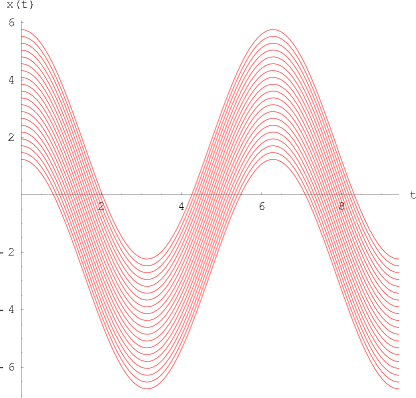
Figure 3: Quantum trajectories for harmonic oscillator computed using derivative propagation approach.

The solid curve in Fig. 4 shows the time correlation function of the wavefunction and its Fourier transform. Here, we performed the calculation out to $t=20\pi$ corresponding to 10 complete oscillation cycles. Both $C(t)$ and its spectral representation $\tilde{C}(\omega)$ agree perfectly with analytical results with $\tilde{C}(\omega)$ accurately mapping out the harmonic progression of the energy levels in this well $\omega_{n}=\omega(n+1/2)$ as well as the expansion coefficients for the projection of the initial wavefunction on to the eigenstates of the well, $c_{n}=|\langle n|\psi_{o}\rangle|^{2}$. For the case at hand, the first 4 coefficients are $c=\{0.606531,0.303265,0.0758163,0.0126361\}$ and agree nicely with the roughly 8:4:1 ratio of the first three peaks in $C(\omega)$.

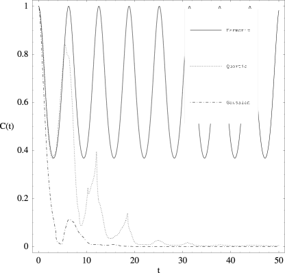
Figure 4: Correlation function and its spectral representation for a gaussian wavepacket in various potentials computed using Bohm-IVR/derivative propagation approach. (Key: $-$ = Harmonic ($V_{HO})$; $\cdot\cdot\cdot=$ Quartic, ($V_{QO}$); $-\cdot-$=Gaussian well ($V_{G}$).)

IV.2 Quartic Perturbed Harmonic

In this case, we apply a slight anharmonic squeeze to the harmonic well. In an anharmonic system, an initial gaussian wave function retains its gaussian form for short period of time before bifurcating into a multitude of components due to interferences. Such features are most likely to occur where the underlying classical trajectory crosses a conjugate or focal point. Such crossings are strictly forbidden for quantum Bohmian trajectories and lead to rapidly varying quantum forces over a short spatial region. Consequently, interference effects in anharmonic systems has proven to be somewhat of a bugbear for implementing quantum trajectory approaches based upon fitting the quantum potential (and its derivatives) to a simple polynomial over a set of quantum trajectories.

The derivative propagation trajectories also retain their coherences for a short period of time. However, after only one or two oscillations, crossings become more frequent and the ensemble of trajectories degrades into an incoherent mess. Had we performed this with the moving-weighted least squares (MWLS) or other methods which extracts the quantum potential from an ensemble of trajectories, the results would have been cataclysmic. Our experience has indicated that even small errors in constructing the quantum force from the ensemble can lead to a rapid amplification of error in the propagation. Remarkably, even though the ensemble has apparently lost coherence amongst its members, the individual trajectories exhibit non-classical deflections, and quasi-periodic behavior one expects from truly quantum trajectories.

Turning towards the autocorrelation and its Fourier transform. $C(t)$ shows some recurrences at $t\approx 2\pi n$ as in the harmonic case, but these rapidly die out after 5-6 beats. This limits our ability to resolve the eigenenergies in the Fourier transform. Nonetheless, at least 4 peaks can be distinguished.

IV.3 Inverted Gaussian Potential

In this final example, $V_{G}$ is an inverted gaussian and supports only two eigenstates (at $E=-0.59386$ and $E=-0.0356576$). In this example we used 30 trajectories since the majority of the trajectories near the leading edges of the distribution leave the potential region almost immediately. In Fig. 5 we show 10 trajectories that started in the center of the initial wavepacket. As time progresses, many of these eventually escape the potential well leaving only one of the original 30 trajectories in the well.

The long-time accuracy of the ensemble is not so important since we are ultimately interested in computing $C(t)$. This we show in Fig. 4 along with its Fourier transform. One can clearly identify 6 recursion peaks spaced roughly every 0.35 ps. These correspond to the nearly harmonic motion of the trajectories closest to the center of the ensemble.

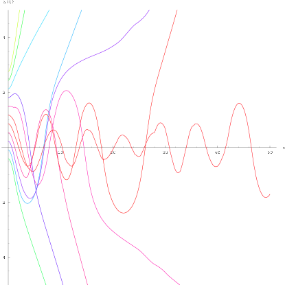
Figure 5: Quantum trajectories for inverted gaussian well example.

V Discussion

For low dimensional systems, there are arsenals of robust and computationally efficient methodologies for computing exact quantum dynamics for both time dependent and time-independent systems. However, these methods are severely limited by dimensionality since the computational effort and storage required to perform an exact quantum calculation increases almost exponentially with dimensionality. Thus, approximate methods, such as those introduced here, provide a viable path way towards higher dimensions with increasing complexity. While we have focused entirely upon one-dimensional examples, the Bohm-IVR and derivative propagation equations are exact and can be easily implemented in a multi-dimensional setting.

What do the individual trajectories mean? Are the trajectories computed via the derivative propagation methods really Bohm trajectories? The answer, I believe is a definite yes and no. Yes, they are Bohm trajectories, but not for a initial single gaussian wavepacket evolving in a given potential. They correspond to trajectories arising from a diverging set of wave functions where each wave function component is constrained to have a particular functional form dictated by truncating the hierarchy. In essence, by truncating the hierarchy, one introduces dephasing and decoherence into the dynamics of a quantum system. This is evident in the time-correlation function for the particle in the harmonic + quartic potential. The time correlation function for a fully coherent wavepacket should show stronger recurrences and eventually be able to resolve the eigenenergies of the system upon Fourier transform. One evidence for this is that for bound systems other than the harmonic oscillator, the autocorrelations we compute using the derivative propagation decay to zero after a few recurrences, and never recover coherence.

For exact quantum mechanics, this implicit loss of coherence at long-times clearly undesirable. However, for condensed phase systems, especially in cases where we have a low dimensional quantum subsystem in contact with a high-dimensional “bath” of oscillators, reduction of the density matrix of the subsystem to a gaussian form in the coherences occurs spontaneously due to decoherence. maddox ; irene3 ; irene4 . Consequently, so long as the “physical” decoherence time is smaller than the “truncation induced ” decoherence time, time-correlation functions computed using the Bohm-IVR approach we describe herein are expected to quite accurate.

- (1) B. K. Dey, A. Askar, and H. Rabitz, J. Phys. Chem. 109, 8770 (1998).
- (2) C. L. Lopreore and R. E. Wyatt, Phys. Rev. Lett. 82, 5190-5193 (1999).
- (3) F. Sales Mayor, A. Askar, and H. A. Rabitz, J. Chem. Phys. 111, 2423-2435 (1999).
- (4) E. R. Bittner J. Chem. Phys. 112, 9703 (2000).
- (5) R. E. Wyatt and E. R. Bittner, J. Chem. Phys. 113, 8898-8907 (2000).
- (6) E. R. Bittner and R. E. Wyatt, J. Chem. Phys. 113, 8888 (2000).
- (7) J. B. Maddox and E. R. Bittner, Phys. Rev. E 65, 026143 (2002).
- (8) J. Maddox and E. R. Bittner, J. Phys. Chem. 106, 7981 (2002).
- (9) I. Burghardt and L. Cederbaum, J. Chem. Phys. 115, 10312 (2001).
- (10) I. Burghardt and L. Cederbaum, J. Chem. Phys. 115, 10303 (2001).
- (11) E. R. Bittner, J. Maddox, and I. Burghardt, Int. J. Quant. Chem. 89 , 313-321 (2002).
- (12) Irene Burghardt and Klaus B. Møller J. Chem. Phys. 117, 7409 (2002).
- (13) K. H. Hughes and R. E. Wyatt, Chem. Phys. Lett. 366, 336-342 (2002).
- (14) C. Trahan and R. E. Wyatt, J. Chem. Phys., in press (2003).
- (15) R. E. Wyatt and E. R. Bittner, Comp. in Sci. and Eng. (in press 2003).
- (16) J. B. Maddox and E. R. Bittner, Estimating Bohm s quantum potential using Bayesian computation, J. Chem. Phys., to be submitted (2003).
- (17) N. Makri and Y. Zhao, J. Chem. Phys. in press (2003).
- (18) D. Bohm, Phys. Rev. 85, 167-179 (1952).
- (19) L . de Broglie, C. R. Acad. Sci. paris 183, 447 (1926).
- (20) P. R. Holland, The Quantum Theory of Motion, (Cambridge University Press, 1993).
- (21) C. Trahan, K. Hughes and R. E. Wyatt, J. Chem. Phys, in press (2003).
- (22) S. Garashchuk and V. A. Rassolov J. Chem. Phys. 118, 2482 (2003).
- (23) M. S. Child and D. V. Shalashilin,J. Chem. Phys. 118, 2061 (2003)
- (24) Takeshi Yamamoto and William H. Miller J. Chem. Phys. 118, 2135 (2003)
- (25) J. H. Van Vleck, Proc. Nat. Acad. Sci. US 14, 178 (1928).
- (26) M. F. Herman and E. Kluk, Chem. Phys. 91, 27 (1984).
- (27) E. Kluk, M. F. Herman, and H. L. Davis, J. Chem. Phys. 84, 326 (1986).
- (28) M. F. Herman, J. Chem. Phys. 85, 2069 (1986).
- (29) J. C. Burant and V. S. Batista, J. Chem. Phys. 116, 2748 (2002).
- (30) Nancy Makri and William H. Miller, J. Chem. Phys. 116, 9207 (2002).
- (31) Sophya Garashchuk and John C. Light, J. Chem. Phys. 113, 9390 (2000).