Geometrical Conditions for CPTP Maps and their Application to a Quantum Repeater and a State-dependent Quantum Cloning Machine

Abstract

We address the problem of finding optimal CPTP (completely positive, trace preserving) maps between a set of binary pure states and another set of binary generic mixed state in a two dimensional space. The necessary and sufficient conditions for the existence of such CPTP maps can be discussed within a simple geometrical picture. We exploit this analysis to show the existence of an optimal quantum repeater which is superior to the known repeating strategies for a set of coherent states sent through a lossy quantum channel. We also show that the geometrical formulation of the CPTP mapping conditions can be a simpler method to derive a state-dependent quantum (anti) cloning machine than the study so far based on the explicit solution of several constraints imposed by unitarity in an extended Hilbert space.

I Introduction

Suppose that we receive a quantum state which is drawn from a parametrized set $\{\hat{f}_{i}\}$ with known a priori probabilities, $\{p_{i}\}$, and that we have another set of states $\{\hat{g}_{i}\}$, which we call templates, at our disposal. Our task is to output an appropriate state function of the templates that best matches the input. The meaning of best matching depends on the task that we are going to pursue. For example, we may consider an eavesdropping strategy in a quantum cryptosystem, an action of a quantum repeater in a communication channel, a state-dependent cloning process, and so on.

The best matching process is generally described by a completely positive trace preserving (CPTP) map from the input to the output state sets. Unfortunately, however, the problem of finding the optimal CPTP mapping between given sets of quantum states is still poorly understood. For example, the necessary and sufficient conditions for the existence of a CPTP mapping between generic mixed states are known only for binary sets of states in a two dimensional space, $\{\hat{f}_{1},\hat{f}_{2}\}$ and $\{\hat{g}_{1},\hat{g}_{2}\}$ albertiuhlmann (with $\hat{g}_{i}\equiv[\hat{I}+\vec{g_{i}}\cdot\hat{\sigma}]/2$ and, without lack of generality, $\vec{g_{1}}^{2}=\vec{g_{2}}^{2}=g^{2}$, and $g\in[0,1]$). This result has never been exploited for practical purposes of quantum information processing.

In this paper, we derive a simple geometrical framework for the general theorem on the existence of CPTP mappings, and then apply it to the problem of designing a quantum optimal repeater for relaying classical information over a lossy quantum channel, and to describe a special kind of state-dependent quantum cloning machine.

Let us suppose that we are at an intermediate station and receive very weak coherent states $\hat{f}_{1}=\left|\alpha\right\rangle\left\langle\alpha\right|$ and $\hat{f}_{2}=\left|-\alpha\right\rangle\left\langle-\alpha\right|$ and that we must replace these weak signals with stronger ones consisting of the templates $\hat{g}_{1}=\left|\beta\right\rangle\left\langle\beta\right|$ and $\hat{g}_{2}=\left|-\beta\right\rangle\left\langle-\beta\right|$ (where the strict inequality $|\beta|>|\alpha|$ holds) to improve the transmission performance through the second channel which is assumed to be lossy.

We consider CPTP mappings from the inputs to not only the given template elements but also a classical mixture of them. This setting is especially motivated by a practical scenario where one should find appropriate repeating states for the second lossy channel and design the optimal mapping for outputting those states. Actually, such states will be more or less semi-classical ones based on Gaussian states because there will be no much merit to use any non-classical states for a long-haul lossy channel, as non-classical states will decohere rapidly and result in semi-classical ones. What remains in practice is then to find an appropriate mixture of coherent state templates. Thus, we are to design the optimal CPTP map acting on the input $\hat{f}_{i}$, that outputs a quantum state $\hat{\rho}_{i}$ of the form

$$\hat{f}_{i}\mapsto\hat{\rho}_{i}=\sum_{j}p_{ij}\hat{g}_{j}.$$ (1)

Another ansatz is then that of quantum cloning. We are concerned with the special case where, given $N$ identical inputs $\hat{f}_{i}^{\otimes N}$, we are only able to construct outputs which are classical mixtures of the templates consisting of $M$ copies $\hat{g}_{i}^{\otimes M}$. This is a more restricted model than the ones studied in the literature to date. However, as seen in section IV, our model provides a reasonable cloning performance compared with that of more general models known so far. In particular, when one considers the use of quantum cloning for a lossy quantum channel based on Gaussian states, our model can be a good practical scenario as mentioned in the previous paragraph. An advantage of our method is that we just have to maximize the chosen figure of merit along a certain curve specifying the boundary of the allowed CPTP mappings, unlike the conventional methods that rely on dealing with all the inequalities for the constraints imposed by unitarity over extended Hilbert spaces with ancilla.

II CPTP Mapping Existence Condition

The necessary and sufficient conditions for the existence of a CPTP mapping between the sets of 2-dim states derived by Alberti and Uhlmann albertiuhlmann are expressed in the form

$$d_{tr}(\hat{f}_{1},t\hat{f}_{2})\geq d_{tr}(\hat{\rho}_{1},t\hat{\rho}_{2})~{}~{}~{};~{}~{}~{}\forall t\in{\cal{R}^{+}},$$ (2)

where the trace norm distance between two operators $\hat{A}$ and $\hat{B}$ is defined as $d_{tr}(\hat{A},\hat{B})\equiv{\rm\,Tr}\,[(\hat{A}-\hat{B})^{\dagger}(\hat{A}-\hat{B})]^{1/2}$.

Let us then write the output states as

$$\hat{\rho}_{1} = p\left|g_{1}\right\rangle\left\langle g_{1}\right|+(1-p)\left|g_{2}\right\rangle\left\langle g_{2}\right|,$$

$$\hat{\rho}_{2} = q\left|g_{2}\right\rangle\left\langle g_{2}\right|+(1-q)\left|g_{1}\right\rangle\left\langle g_{1}\right|,$$ (3)

with the output probabilities $(p,q)\in[0,1]$. The above condition Eq. (2) implies a complicated set of constraints on the parameters describing generical mixed input and output states, and on the probability distributions $p,q$, but it can be explicitly calculated within a nice geometrical framework.

In particular, in the most general model of mixed ‘initial’ and ‘template’ states defined by an arbitrary vector in the Bloch sphere, $\hat{f}_{i}\equiv[\hat{I}+\vec{f_{i}}\cdot\hat{\sigma}]/2$ and $\hat{g}_{i}\equiv[\hat{I}+\vec{g_{i}}\cdot\hat{\sigma}]/2$, respectively, Alberti and Uhlmann’s condition can be rewritten as

$$h(\hat{p},\hat{q};\vec{f_{i}},\vec{g_{i}};t) \equiv h^{B}-|h^{B}|$$ (4)

$$- R(h^{A}-|h^{A}|)\geq 0~{}~{}~{};~{}~{}~{}\mbox{$\forall t\in{\cal R}^{+}$}$$

where, using the new coordinates $\hat{p}\equiv p-1/2$, $\hat{q}\equiv q-1/2$ ($(\hat{p},\hat{q})\in[-1/2,1/2]$) to simplify the notation, we have introduced the parabolic functions of $t$ as

$$h^{A}(X;t) \equiv X-2(2+X)t+Xt^{2}$$

$$h^{B}(\hat{p},\hat{q};Y_{0};t) \equiv (Y_{0}-4\hat{p}^{2})-2(Y_{0}+4\hat{p}\hat{q})t$$ (5)

$$+ (Y_{0}-4\hat{q}^{2})t^{2},$$

and the parameters

$$R \equiv {f^{2}\sin^{2}\phi\over g^{2}\sin^{2}\theta}~{}\geq 0,$$

$$X \equiv {1-f^{2}\over f^{2}\sin^{2}\phi}~{}\geq 0,$$

$$Y_{0} \equiv 1+{1-g^{2}\over g^{2}\sin^{2}\theta}~{}\geq 1,$$ (6)

with $2\sin^{2}\theta\equiv 1-\vec{g_{1}}\cdot\vec{g_{2}}/g^{2}$, $~{}2\sin^{2}\phi\equiv 1-\vec{f_{1}}\cdot\vec{f_{2}}/f^{2}$ and $\phi,\theta\in[0,\pi]$.

Now let us turn to the analysis of condition (4). This can be seen to reduce to the following constraints

$$\Delta t_{+} \equiv t_{+}^{A}-t_{+}^{B}\geq 0,$$

$$\Delta t_{-} \equiv t_{-}^{B}-t_{-}^{A}\geq 0,$$ (7)

where $t^{A}_{\pm}$ and $t^{B}_{\pm}$ are the zeros of $h^{A}$ and $h^{B}$, respectively, and

$$H(\hat{p},\hat{q},R,X,Y_{0};t) = (Y_{0X}-4\hat{p}^{2})-2[Y_{2X}+4\hat{p}\hat{q}]t$$ (8)

$$+ (Y_{0X}-4\hat{q}^{2})t^{2}\geq 0~{}~{}~{};$$

$$~{}~{}\mbox{for $t_{-}^{B}\leq t\leq t_{+}^{B}$},$$

where, for ease of presentation, we have defined $Y_{nX}\equiv Y_{0}-(n+X)R$. After some algebra and the analysis of a few geometrical constraints in the parameter space $(p,q)$, one finally obtains that the Alberti-Uhlmann condition can be satisfied in certain geometrically simple $(p,q)$ parameter regions, classified according to the values of $R,X$ and $Y_{0}$ (see Appendix).

III Repeater in Lossy Quantum Channel

In the model for the repeater in a quantum lossy channel, the input states are pure, and the Alberti and Uhlmann condition can be greatly simplified as the well known fidelity criterion uhlmann

$$F(\hat{f}_{1},\hat{f}_{2})\leq F(\hat{\rho}_{1},\hat{\rho}_{2}).$$ (9)

Given the output states (3), it is easy to evaluate the fidelities so that the CPTP mapping existence condition (9) can be explicitly rewritten as

$$pq+(1-p)(1-q)-R\leq 2\sqrt{p(1-p)q(1-q)},$$ (10)

where we have introduced the parameters

$$R\equiv\frac{1-\kappa^{2}}{1-K^{2}}<1,\quad\kappa\equiv\langle\alpha|-\alpha\rangle,\quad K\equiv\langle\beta|-\beta\rangle.$$ (11)

The inequality (10) is trivially satisfied when its l.h.s. is negative definite, i.e. when

$$q \geq {1\over 2}\left[{2R-1\over 2p-1}+1\right]\quad(0<p<{1\over 2}),$$ (12)

$$q \leq {1\over 2}\left[{2R-1\over 2p-1}+1\right]\quad({1\over 2}<p<1).$$ (13)

Otherwise,

$$\Delta(p,q)\equiv(p+q+R-1)^{2}-4Rpq\leq 0,$$ (14)

should hold. Collecting these two cases together, we finally conclude that the CPTP mapping existence condition (10) is satisfied for the range of parameters $(p,q)$ contained within the shaded area shown in Fig. 1. The upper boundary is specified by

$$\begin{array}[]{ll}q&=1\qquad\qquad(0\leq p\leq R),\\ q&=1-R-(1-2R)p+2\sqrt{R(1-R)p(1-p)}{}\\ {}&\qquad\qquad\qquad(R\leq p\leq 1),\\ 0&\leq q\leq R\qquad(\mathrm{at}\quad p=1),\end{array}$$ (15)

while the lower boundary is given by

$$\begin{array}[]{ll}1&-R\leq q\leq 1\qquad(\mathrm{at}\quad p=0),\\ q&=1-R-(1-2R)p-2\sqrt{R(1-R)p(1-p)}{}\\ {}&\qquad\qquad\qquad(0\leq p\leq 1-R),\\ q&=0\qquad\qquad(1-R\leq p\leq 1).\end{array}$$ (16)

Figure 1: The allowed $(p,q)$ region (shaded area) for the existence of a CPTP mapping between two input pure states and two output mixed states ($R=0.25$).

III.1 Optimal Repeater

Now we apply the above results to derive the optimal repeater for the second channel which is assumed to be a simple lossy channel described by

$$\hat{\cal L}(\left|\pm\gamma\right\rangle\left\langle\pm\gamma\right|)=\left|\pm\eta\gamma\right\rangle\left\langle\pm\eta\gamma\right|,$$ (17)

for any coherent state $\left|\gamma\right\rangle$ and $0<\eta<1$. We consider two kinds of measures of the transmission performance through the lossy channel, i.e. the average bit error rate $P_{\mathrm{e}}$ and the Holevo capacity $\chi({\cal E})$ for the output ensemble from the channel, ${\cal E}=\{\hat{\rho}_{1}^{\prime},\hat{\rho}_{2}^{\prime};1-\xi,\xi\}$, where $\hat{\rho}_{i}^{\prime}\equiv\hat{\cal L}(\hat{\rho}_{i})$ and

$$\hat{\rho}_{1} \equiv p\left|\beta\right\rangle\left\langle\beta\right|+(1-p)\left|-\beta\right\rangle\left\langle-\beta\right|,$$

$$\hat{\rho}_{2} \equiv q\left|-\beta\right\rangle\left\langle-\beta\right|+(1-q)\left|\beta\right\rangle\left\langle\beta\right|,$$ (18)

$1-\xi$ and $\xi$ being the a priori probabilities for $\hat{\rho}_{1}^{\prime}$ and $\hat{\rho}_{2}^{\prime}$, respectively, as well as for $\left|\alpha\right\rangle$ and $\left|-\alpha\right\rangle$.

We first consider minimizing the average error probability $P_{\mathrm{e}}$ with respect to a POVM $\{\hat{\Pi}_{1},\hat{\Pi}_{2}\}$

$$P_{\mathrm{e}}^{\mathrm{min}} \equiv \min_{\{\hat{\Pi}_{1},\hat{\Pi}_{2}\}}\left[(1-\xi){\rm\,Tr}\,(\hat{\Pi}_{1}\hat{\rho}_{1}^{\prime})+\xi{\rm\,Tr}\,(\hat{\Pi}_{2}\hat{\rho}_{2}^{\prime})\right]$$ (19)

$$= 1-\xi+\min_{\hat{\Pi}_{1}}\left[{\rm\,Tr}\,(\hat{\Pi}_{1}\hat{\Lambda})\right],$$

where $\hat{\Lambda}\equiv\xi\hat{\rho}_{2}^{\prime}-(1-\xi)\hat{\rho}_{1}^{\prime}$ and we have used the property $\hat{\Pi}_{1}+\hat{\Pi}_{2}=\hat{I}$. The minimum error is then found by taking $\hat{\Pi}_{1}=\left|\lambda_{-}\right\rangle\left\langle\lambda_{-}\right|$, where $\left|\lambda_{-}\right\rangle$ is the negative eigenvalue eigenstate of the operator $\hat{\Lambda}$. We then have

$$P_{\mathrm{e}}^{\mathrm{min}}(p,q) = {1\over 2}\Biggl{\{}1-\biggl{[}(2\xi-1)^{2}K^{\prime 2}$$ (20)

$$+ [2\xi q+2(1-\xi)p-1]^{2}(1-K^{\prime 2})\biggr{]}^{1\over 2}\Biggr{\}},$$

with $K^{\prime}\equiv\langle\eta\beta|-\eta\beta\rangle$. So clearly we are to find the optimal repeater maximizing the quantity

$$S(p,q)\equiv\xi q+(1-\xi)p.$$ (21)

Since the latter is an increasing function in both $p$ and $q$, it can be maximized under the CPTP map existence constraints by use of the standard Lagrange multiplier method, i.e. by solving the following set of equations

$$\nabla S(p,q)=\lambda\nabla[\Delta(p,q)]~{}~{}~{};~{}~{}~{}\Delta(p,q)=0,$$ (22)

where $\lambda$ is a constant. Solving Eqs. (22) with the aid of Eq. (14) and Fig. 1, it is readily shown that the optimal bit error rate is obtained for:

$$p_{\mathrm{opt}}={1\over 2}\left[1+{c_{-}\over\sqrt{c}}\right]~{}~{}~{};~{}~{}~{}q_{\mathrm{opt}}={1\over 2}\left[1+{c_{+}\over\sqrt{c}}\right],$$ (23)

for $0<R<1$ and $0<\xi<1$, where

$$c_{\pm} \equiv R\pm(2\xi-1)(1-R),$$

$$c \equiv 1-4\xi(1-\xi)(1-R).$$ (24)

Furthermore, for the optimal pair (23) we have

$$S_{\mathrm{opt}}=C+D[\sqrt{c}-1]/2.$$ (25)

Note that in the particular case of equiprobably distributed inputs, i.e. when $\xi=1/2$, we have that $c_{+}=c_{-}=c=R$ and then the optimal point for $0<R<1$ explicitly reads $p_{\mathrm{opt}}=q_{\mathrm{opt}}=(1+\sqrt{R})/2$.

With $(p,q)$ evaluated as the optimal pair (23) we get

$$P_{\mathrm{e,CPTP}}^{\mathrm{min}}={1\over 2}\{1-\sqrt{1-4\xi(1-\xi)[1-(1-K^{\prime 2})R]}\}.$$ (26)

We compare this with the average bit error rate in the case of no action by the repeater, i.e. with final states given by $\left|\pm\eta\alpha\right\rangle\left\langle\pm\eta\alpha\right|$, which is expressed by

$$P_{\mathrm{e,NOACT}}\equiv[1-\sqrt{1-4\xi(1-\xi)\kappa^{\prime 2}}]/2.$$ (27)

where $\kappa^{\prime}\equiv\langle\eta\alpha|-\eta\alpha\rangle$. As it can be simply proved and directly seen from Fig. 2, the optimal error probability $P_{\mathrm{e,CPTP}}^{\mathrm{min}}$ is always smaller than $P_{\mathrm{e,NOACT}}$ for any choice of initial probability distributions $\xi$, $0<\eta<1$ and $|\beta|>|\alpha|$. That is, the intermediate action of the repeater with optimal CPTP mapping on the initial states reduces the final error probability of detecting the original states.

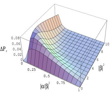
Figure 2: The difference in the error probabilities for Bob, $\Delta P_{\mathrm{e}}\equiv P_{\mathrm{e,NOACT}}-P_{\mathrm{e,CPTP}}^{\mathrm{min}}$, as a function of $|\alpha/\beta|^{2}$ and $|\beta|^{2}$ in the case $\eta=1/\sqrt{2}$, $\xi=1/2$.

Now we turn our attention to the problem of maximizing the Holevo capacity

$$\chi({\cal E})\equiv S(\hat{\rho}^{\prime})-\sum_{k}\xi_{k}S(\hat{\rho}_{k}^{\prime})=\sum_{k}\xi_{k}D(\hat{\rho}_{k}^{\prime}||\hat{\rho}^{\prime}),$$ (28)

where $\hat{\rho}^{\prime}=\sum_{k}\xi_{k}\hat{\rho}_{k}^{\prime}$, $S(\hat{\rho}^{\prime})$ is the von Neumann entropy, and $D(\hat{\rho}_{k}^{\prime}||\hat{\rho}^{\prime})$ is the relative entropy. First notice that $\chi({\cal E})$ is maximized at the extreme points of the convex set $(p,q)$ of the region allowed by the Alberti-Uhlmann condition, because $\chi({\cal E})$ is a downward convex function with respect to the pair $(p,q)$. In fact, let $(p_{\mathrm{E}},q_{\mathrm{E}})$ and $(p_{\mathrm{A}},q_{\mathrm{A}})$ be extreme and interior points, respectively. Define the corresponding ensembles as ${\cal E}^{\mathrm{E}}=\{\hat{\rho}_{k}^{\mathrm{E}};\xi_{k}\}$ and ${\cal E}^{\mathrm{A}}=\{\hat{\rho}_{k}^{\mathrm{A}};\xi_{k}\}$. Then for another interior point,

$$\hat{\rho}_{k}^{\mathrm{B}}=(1-\zeta)\hat{\rho}_{k}^{\mathrm{E}}+\zeta\hat{\rho}_{k}^{\mathrm{A}}$$ (29)

(where $0<\zeta<1$), we have

$$\chi({\cal E}^{\mathrm{B}})\leq(1-\zeta)\chi({\cal E}^{\mathrm{E}})+\zeta\chi({\cal E}^{\mathrm{A}}),$$ (30)

due to the joint convexity of the relative entropy.

The problem of maximization of the Holevo capacity $\chi_{\mathrm{CPTP}}$ along the (elliptic) boundary of the CPTP allowed region in the $(p,q)$ parameter space for general initial probability distributions $\xi$ is still quite cumbersome but can be solved numerically. For the sake of clarity we explicitly show here a practical case of equiprobably distributed inputs, $\xi=1/2$ (maximum amount of information encoded in the inputs). It is quite easy to check that in this case the channel capacity is zero along the line $q=1-p$ and symmetric with respect to the lines $q=p$ and $q=1-p$, and monotonically increasing towards the points $(1,1)$ and $(0,0)$. In particular, its maximum is achieved at the optimal point $p_{\mathrm{opt}}=q_{\mathrm{opt}}=(1+\sqrt{R})/2$ on the boundary of the allowed region. Its behaviour as a function of $\kappa$ is shown in Fig. 3, where it is also compared with the channel capacity

$$\chi_{\mathrm{NOACT}}\equiv-(\lambda_{\kappa+}\log\lambda_{\kappa+}+\lambda_{\kappa-}\log\lambda_{\kappa-})$$ (31)

(with $\lambda_{\kappa\pm}\equiv(1\pm\kappa)/2$) for the case of no action by the repeater and the Holevo bound for the input states, i.e.

$$\chi_{\mathrm{INPUT}}\equiv-(\lambda_{\kappa^{\prime}+}\log\lambda_{\kappa^{\prime}+}+\lambda_{\kappa^{\prime}-}\log\lambda_{\kappa^{\prime}-})$$ (32)

(with $\lambda_{\kappa^{\prime}\pm}\equiv(1\pm\kappa^{\prime})/2$).

Figure 3: The Holevo capacities $\chi_{\mathrm{CPTP}}$ (dashed line), $\chi_{\mathrm{NOACT}}$ (dotted line) and $\chi_{\mathrm{INPUT}}$ (continuous line) as a function of the inputs overlap $\kappa$ for the equiprobable inputs case ($\xi=1/2$), $|\beta/\alpha|=2$ and $\eta=1/\sqrt{2}$.

As one can see, there are both parameter ($\beta/\alpha,\eta$) regions where $\chi_{\mathrm{CPTP}}>\chi_{\mathrm{NOACT}}$ and $\chi_{\mathrm{CPTP}}<\chi_{\mathrm{NOACT}}$. In particular, defining $\kappa_{0}$ as the intercept point between the curves $\chi_{\mathrm{CPTP}}$ and $\chi_{\mathrm{NOACT}}$ (i.e. such that $\chi_{\mathrm{CPTP}}(\kappa_{0})\equiv\chi_{\mathrm{NOACT}}(\kappa_{0})$), for $0<\kappa<\kappa_{0}<1$ the accessible information is bigger when amplifying the signals at the repeater, while for $\kappa_{0}<\kappa<1$ the best performance is obtained without amplification. This behavior can be explained as follows: for small $\kappa$ the inputs tend to be more orthogonal and the quantum repeater helps; on the other hand, for larger $\kappa$, the inputs tend to overlap and there is no gain in using the quantum repeater. Furthermore, one can easily check that, as $\eta$ decreases (the channel becomes more lossy), although the absolute channel capacity performance decreases, the range of $\kappa$ for which $\chi_{\mathrm{CPTP}}>\chi_{\mathrm{NOACT}}$ also becomes larger ($\kappa_{0}$ increases): for very noisy channels the amplification by the repeater is essential even for the case when the inputs are almost completely overlapping.

The different behavior measured by the minimum bit error rate and the Holevo capacity may be also interpreted as follows: the Helstrom bound specifies the performance of a single shot measurement on each signal state, while the Holevo capacity is a measure for the coding by a large scale collective measurement where the coherence involved in sequences of signal states must be fully used to extract as much information as possible. So, preparing mixed state signals at the repeater could spoil in some cases the coherence involved in sequences of pure state signals $|\pm\eta\alpha\rangle$, leading to the reduction of the Holevo capacity.

For the near future optical communications based on classical coding, the bit error rate is of greater interest, and the optimal repeater derived here will be useful. When the template states $\{|\beta\rangle,|-\beta\rangle\}$ can be prepared with enough power such as $K\sim 0$, then the optimal repeating strategy is simply realized by the intercept-resend (IR) strategy. That is, we first discriminate $\{|\beta\rangle,|-\beta\rangle\}$ by the minimum error measurement, and then assign an appropriate template state based on the measurement results. In the case of $\xi=1/2$, the repeating states are specified by Eq. (18) with the parameters

$$p=q={1\over 2}\left(1+\sqrt{1-\kappa^{2}}\right),$$ (33)

and the final bit error rate is

$$P_{\mathrm{e,IR}}^{\mathrm{min}}={1\over 2}\{1-\sqrt{(1-\kappa^{2})(1-K^{\prime 2})]}\}.$$ (34)

Figure 4: The network which realizes the optimal CPTP mapping for the repeater, with ${\hat{U}}_{ab}\equiv\exp\{\left|0\right\rangle_{a}\left\langle 1\right|[\theta_{-}\left|0\right\rangle_{b}\left\langle 1\right|+\theta_{+}\left|1\right\rangle_{b}\left\langle 0\right|]-\mathrm{h.c.}\}$.

When, on the other hand, the non-orthogonality of the template states should be taken into account, we have to consider quantum processes which do not include any intermediate measurement process. One possible implementation is given by the quantum network shown in Fig. 4. The computational basis is made up of the so called even and odd coherent states,

$$|0\rangle \equiv {1\over\sqrt{2(1+\kappa)}}(|\alpha\rangle+|-\alpha\rangle),$$

$$|1\rangle \equiv {1\over\sqrt{2(1-\kappa)}}(|\alpha\rangle-|-\alpha\rangle).$$ (35)

The controlled rotations are defined by

$$\hat{R}(\theta_{\pm})\equiv\left(\begin{array}[]{cc}\cos\theta_{\pm}&-\sin\theta_{\pm}\\ \sin\theta_{\pm}&\cos\theta_{\pm}\end{array}\right),$$ (38)

where $\theta_{\pm}\equiv(\arcsin K/\kappa\pm\pi/2)/2$. The ancilla qubit is initialized in the even coherent state $|0\rangle_{b}$, where the subscript $b$ refers to a particular mode of the coherent template states. The repeating states are simply obtained at the output port in mode b by tracing out the states in mode $a$. Unfortunately, this type of quantum circuit still requires hypothetical non-linear processes to generate the even and odd coherent states as well as the cross Kerr effect between mode a and b sasaki ; Cochrane99 .

IV State-dependent Quantum Cloning

Another interesting application of the CPTP mapping results is in state-dependent cloning. As it is well known, an arbitrary unknown quantum state cannot be cloned wootterszurek . It is possible, however, to produce imperfect copies of quantum states, both deterministically (when the cloning machine can only perform unitary operations) and probabilistically (where via postselection measurements in an ancillary space, faithful copies of the input are obtained with non zero success probability). Several results on quantum cloning are already known by now (for a selected, though not exhaustive, bibliography, see, e.g., Refs. fanmatsumotowadati ).

In this section we will exploit the geometric results concerning the existence of a CPTP map between 2-d quantum systems section to describe an $N\rightarrow M$ (anti) cloning state-dependent machine. In particular, we assume that the input states are pure and given as an $N$-fold tensor product $\left|f_{i}\right\rangle^{\otimes N}$, while the ‘templates’ $\hat{g}_{i}$ are pure ($g=1$) and $M$-copies clones ($M\geq N\geq 1$) of the input states $\left|f_{i}\right\rangle$, i.e.

$$\left|f_{i}\right\rangle\rightarrow\left|\tilde{f}_{i}\right\rangle\equiv\left|f_{i}\right\rangle^{\otimes N}~{}~{}~{};~{}~{}~{}\left|g_{i}\right\rangle\equiv\left|f_{i}\right\rangle^{\otimes M}.$$ (39)

We then restrict our analysis to the special case in which we assumed that we are only able to construct outputs which are classical mixtures of these templates, that is the outputs are given again by Eq. (3). More general cloner models (including the state-dependent copiers which unitarily map pure initial states to a pure state superposition of clones as in Refs. bruss1 ; chefles2 ) will be considered elsewhere. In our ansatz, then, it is straightforward to see, by using the Bloch sphere parametrization for $\hat{g}_{i}$ and noting that the states $\{\left|g_{i}\right\rangle\}$ (as well as the states $\{\left|f_{i}\right\rangle\}$) span a 2-d Hilbert space, that the overlaps must be

$$|\left\langle\tilde{f}_{1}|\tilde{f}_{2}\right\rangle|=\cos^{N}\phi~{}~{};~{}~{}|\left\langle g_{1}|g_{2}\right\rangle|=\cos\theta=\cos^{M}\phi.$$ (40)

The case of pure $\left|g_{i}\right\rangle$ can be also immediately handled within the framework discussed in the previous section provided that we take $Y_{0}=1$ (see Eq. (24)). Therefore, for the parameter $R$ of Eq. (6), we obtain

$$R={1-\cos^{2N}\phi\over 1-\cos^{2M}\phi},$$ (41)

with $R\in[N/M,1]$. In order to evaluate the efficiency of the cloning machine, we can now either choose as the figure of merit the ‘global’ fidelity (see, e.g., Refs. bruss1 ; chefles2 )

$$\bar{F}_{G}\equiv(1-\xi)\left\langle\tilde{f}_{1}|\hat{\rho}_{1}|\tilde{f}_{1}\right\rangle+\xi\left\langle\tilde{f}_{2}|\hat{\rho}_{2}|\tilde{f}_{2}\right\rangle,$$ (42)

which can be easily seen to correspond (taking $g=Y_{0}=1$, and $\theta$ and $R$ as defined in Eqs. (40)-(41)) to

$$\bar{F}_{G}=Z^{M}+(1-Z^{M})[(1-\xi)p+\xi q],$$ (43)

with $Z\equiv\cos^{2}\phi$, and then essentially the same as the score $S(p,q)$ of the previous section, with the same maximum at the optimal points $(p_{opt},q_{opt})$ of Eq. (23), finally giving (note that for cloning, $R<1$, see Eq. (41) and Fig. 2a, and the condition $Y_{0}=1$ also implies that $\xi_{0}=0$):

$$\bar{F}_{G,opt}(Z;\xi, N ,M)=1-{(1-Z^{M})\over 2}$$ (44)

$$\cdot \biggl{[}1-\sqrt{1-4\xi(1-\xi){(Z^{N}-Z^{M})\over(1-Z^{M})}}\biggr{]}.$$

Otherwise, we could choose the ‘local’ fidelity (see, e.g., Refs. bruss1 ; chefles2 )

$$\bar{F}_{L}\equiv(1-\xi)F_{1}(\hat{f}_{1},\hat{f}_{1}^{out})+\xi F_{2}(\hat{f}_{2},\hat{f}_{2}^{out}),$$ (45)

where $F_{i}(\hat{f}_{i},\hat{f}_{i}^{out})$ is the fidelity between the reduced density operator for one single copy of the initial state (i.e., $\hat{f}_{i}$) and the reduced density operator for one single copy of the final state (i.e., $\hat{f}_{i}^{out}$, obtained tracing out any $M-1$ qubits from $\hat{\rho}_{i}$, and which is independent of the choice of the remaining copy). Since the output reduced density operators (cf. Eq. (3)) are given by

$$\hat{f}_{1}^{out} = p\hat{f}_{1}+(1-p)\hat{f}_{2},$$

$$\hat{f}_{2}^{out} = q\hat{f}_{2}+(1-q)\hat{f}_{1},$$ (46)

a short calculation shows that

$$\bar{F}_{L}=Z+(1-Z)[(1-\xi)p+\xi q],$$ (47)

which is again optimized by the parameters of Eq. (23) and finally reads

$$(1-Z^{M})(1-\bar{F}_{L,opt}(Z;\xi,N,M))=$$ (48)

$$(1-Z)(1-\bar{F}_{G,opt}(Z;\xi,N,M)).$$

Since the ‘local’ and ‘global’ fidelities are linearly correlated, it is enough in the following to study the behaviour of one of them, e.g. $\bar{F}_{L}$. First of all, cloning is not allowed for the set of parameters $(p,q)$ outside the shaded region of Fig. 2a. Then, considered as a function of $\xi$, $\bar{F}_{L,opt}$ is further maximized (as expected) for the trivial choices $\xi=0$ or $\xi=1$ (only one ‘input’ state), for which $\bar{F}_{L,opt}=1$. It is also easy to see that the optimal $\bar{F}_{L,opt}(\xi)$ is bounded below by $\bar{F}_{L,opt}(\xi=1/2)$, i.e. for the choice of equiprobabilistically distributed input states $\{\left|f_{i}\right\rangle\}$. This case is important because for $\xi=1/2$ the maximum amount of information is encoded in the input states. It is easily seen that this fidelity is an increasing function of $N$ and a decreasing function of $M$. As a function of $Z$ at fixed $N,M$ it decreases from the maximum $\bar{F}_{L,opt}(Z;1/2,N,M)=1$ at $\phi=0$ (the case for maximally indistinguishable initial states) until it reaches a minimum around $\phi_{min}\geq\pi/4$ (for $N=1$ and $M=2$, at which $\bar{F}_{L,opt}\simeq 0.95$) and then again increases towards $\bar{F}_{L,opt}(Z;1/2,N,M)=1$ at $\phi=\pi/2$ (the case for orthogonal, classical inputs). In the asymptotic case of $M\rightarrow\infty$ the ‘local’ fidelity has a similar shape, with the minimum (for $N=1$) $\bar{F}_{L,opt}=25/27\simeq 0.92$ at $\phi_{min}=\arccos\sqrt{5/9}\leq\pi/4$. The optimal ‘local’ average fidelity $\bar{F}_{L,opt}(Z;1/2,N,M)$ is plotted as a function of $Z$ for $N=1$ and $M=2,\infty$ in Fig. 4. Also note that, in the asymptotic limit of $M\rightarrow\infty$, the ‘global’ fidelity reaches the Helstrom bound

$$2\bar{F}_{\mathrm{Helstrom}}\equiv 1+\left[1-4\xi(1-\xi)\left\langle\tilde{f}_{1}|\tilde{f}_{2}\right\rangle\right]^{1/2},$$ (49)

which is the maximum probability to distinguish the two states $\left|\tilde{f}_{1}\right\rangle$ and $\left|\tilde{f}_{2}\right\rangle$. Quantum cloners with state dependent fidelity were already considered in the literature, see, e.g., Refs. bruss1 ; chefles2 ; buzekhillery1 . One of their most important practical use is for eavesdropping strategies in some quantum cryptographic system. As Fig. 4 shows, our local and global fidelities for $\xi=1/2$ are smaller than, respectively, the optimal eavesdropping strategy fidelity described in Ref. bruss1 and the global one of Ref. chefles2 . As we have already stressed, this is just a consequence of the peculiarity of our output states, which are a classical mixture of the perfect clones $\left|f_{i}\right\rangle^{\otimes M}$, while in Refs. bruss1 ; chefles2 the optimization is over a unitary transformation between arbitrary initial and final pure states. The evident advantage of our optimal CPTP mapping method in a general cloning machine relies in not having to deal with all the inequalities which derive from the constraints on the unitarity of transformations over extended Hilbert spaces with ancilla qubits, as we just have to maximize the chosen figure of merit along a certain curve specifying the boundary of the allowed CPTP mappings between the initial and the output (mixed) states.

Figure 5: The optimal average score $\bar{F}_{opt}(Z;0.5,1,M)$ for the parameters: a) $M=2$ (dotted line); b) $M=\infty$ (continuous line), and the optimal local eavesdropping strategy fidelity $F_{l,3}$ in Eq. (51) of Ref. bruss1 for $N=1$ and $M=2$ (dashed line).

The importance and relation of different ‘quality’ measures for cloning other than fidelity, and for instance the realization that generally copiers quantum optimized with respect to fidelity are not optimal with respect to information transfer measures, and viceversa, was stressed, e.g., in Ref. deuar ; footnote . In particular, another measure of the quality of the performance of our copier can be given in terms of the Holevo bound on the copied information for the reduced density outputs (46), i.e. (for the optimal point given by Eq. (23))

$$I_{H}(Z;\xi,N,M) \equiv S(\sum_{i}p_{i}\hat{f}_{i}^{out})-\sum_{i}p_{i}S(\hat{f}_{i}^{out})$$ (50)

$$= \sum_{\alpha=\pm;i=1,2,3}P_{i}~{}\lambda^{i}_{\alpha}\log\lambda^{i}_{\alpha}$$

where

$$2\lambda_{\pm}^{1} \equiv 1\pm\{[c_{-}^{2}+4\xi^{2}R(1-R)Z]/c\}^{1/2},$$

$$2\lambda_{\pm}^{2} \equiv 1\pm\{[c_{+}^{2}+4(1-\xi)^{2}R(1-R)Z]/c\}^{1/2},$$

$$2\lambda_{\pm}^{3} \equiv 1\pm\{[(1-2\xi)^{2}+4\xi(1-\xi)RZ]/c\}^{1/2},$$ (51)

$P_{1}=1-\xi,P_{2}=\xi,P_{3}=-1$ and $c_{\pm},c$ and $R$ are given, respectively, by Eqs. (24) and (41). This should be compared with the maximum information extractable from the original states, given by

$$I_{H}^{in}(Z;\xi)\equiv S(\sum_{i}p_{i}\hat{f}_{i})=-\sum_{\alpha=\pm}\lambda^{in}_{\alpha}\log\lambda^{in}_{\alpha},$$ (52)

with

$$2\lambda_{\pm}^{in}\equiv 1\pm[(1-2\xi)^{2}+4\xi(1-\xi)Z]^{1/2}.$$ (53)

These figures of merit are shown in Fig. 5 for $\xi=1/2$, $N=1$ and $M=2,\infty$, and compared with the Holevo bound of the Wooters and Zurek model wootterszurek (which, in this sense, is nearly optimal as it allows to extract as much information from the copies as from the originals deuar ).

Figure 6: The Holevo bound on the copied information $I_{H}(Z;0.5,1,M)$, for the parameters $M=2$ (dashed line) and $M=\infty$ (continuous line), compared to the Holevo bound for the Wooters Zurek (WZ) cloner (dot-dashed line) and the maximal information extractable from the input states, $I_{H}^{in}(Z;0.5)$ (dotted line).

Completely similar considerations can be extended to the case in which the input and the template states are, respectively, the coherent states $\left|\pm\alpha\right\rangle$ and $\left|\pm\beta\right\rangle$, just by replacing in the previous formulas for $Z\rightarrow Z_{coh}\equiv|\left\langle\alpha|-\alpha\right\rangle|^{2}=Exp[-4|\alpha|^{2}]$. Furthermore, with the same methods we can also consider a special type of copier called $N\rightarrow K+L$ (with $K+L\geq N$) ‘anti-cloning’ machine songhardy . In this ansatz, a set of unknown ‘input’ states $\{\left|f_{i}\right\rangle^{\otimes N}\}$ is transformed into the tensor product of $K$ copies of the input $\left|f_{i}\right\rangle$ times $L$ copies of a state $\left|-f_{i}\right\rangle\equiv\bar{\beta}_{i}\left|0\right\rangle-\bar{\alpha}_{i}\left|1\right\rangle$ which has opposite spin direction with respect to the input one. This type of cloning is physically interesting for a number of information theoretic reasons (see, e.g., Refs. gisinpopescu ).

The pure ‘templates’ are thus chosen as $\left|g_{i}\right\rangle\equiv\left|f_{i}\right\rangle^{\otimes K}\left|-f_{i}\right\rangle^{\otimes L}$, such that now $|\left\langle g_{1}|g_{2}\right\rangle|=\cos^{K+L}\phi$ and $R=[1-\cos^{2N}\phi]/[1-\cos^{2(K+L)}\phi]$, with $R\in[N/(K+L),1]$. The analysis of the optimal efficiency of the anti-cloning machine then follows similar lines to those of the previous cloning machine case, just provided that one makes the substitution $M\rightarrow K+L$.

V Discussion

We have considered the constraints on the existence of CPTP mappings between two arbitrary initial pure states and two arbitrary final mixed states using Uhlmann’s theorem uhlmann and interpreting them within a simple geometrical picture. Exploiting these results, we then studied the model of a quantum communication channel where a set of coherent states are sent by Alice, eventually transformed by an intermediate repeater who can perform an optimal CPTP mapping and, after going through a lossy channel ${\cal L}$, are finally received by Bob with a certain error probability. We have shown that when the intermediate repeater performs the optimally CPTP mapping, the final error probability is always smaller than in the case when no action is taken at the intermediate stage. In other words, we can have a gain when the optimal mapping strategy is applied to repeat or amplify the input signals in the channel. This is a new and intriguing result for quantum communication, showing the potential relevance of the optimal CPTP mapping strategy.

Furthermore, the optimal CPTP mapping constraints have been used to analyze state-dependent optimal cloners where the output is a classical mixture of exact copies of the initial inputs, and the ‘local’ and ‘global’ fidelity between the copies and the input, and an information theoretic ‘quality’ measure given by the Holevo bound on the mutual information between the density operators for the input and the copies reduced states have been discussed. Although our copiers do not achieve the performance of other state-dependent cloners known in the literature (because of the special choice of our outputs), our results (which are new for the anti-cloning machine case) are still interesting as they show that the CPTP mapping ‘geometrical’ methods are simpler and more direct than the study of the several constraints inherent to the extended Hilbert space approaches. It would be interesting to compare our results on cloning with the conditions discussed in Refs. cerf1 for Pauli cloning machines, which seem to derive, albeit using a different analysis, an intriguely similar geometric picture.

Finally, It should be also mentioned that the use of squeezers has been studied as another kind of repeater for coherent states hirota . In particular, it was shown that by optimizing a cascade of squeezers the communication performance of the coherent state channel can be improved. This method is based on the unitary transformation of the squeezer as a noiseless amplifier. Therefore the state overlap between the signal states is not changed, which meens that the Helstrom bound cannot be improved. However, considering homodyne detection (which is a practical detection scheme with the present technology), the improvement in the signal-to-noise ratio brought by the cascade of the squeezers will be very useful. It would be an interesting problem to study quantum repeaters combining our non-unitary repeater with the squeezer repeater for a lossy channel with homodyne detection.

Appendix A  

The solutions to the constraints (7) and (8) for the variables $p$ and $q$ in terms of the parameters $R,X$ and $Y_{0}$ given by eq. (6) can be summarized, after some lengthy but straightforward algebra, by the geometrical pictures shown in Figs. A1-A7. In particular, the allowed regions for the existence of the CPTP maps between arbitrary mixed initial and final states are the shaded regions in these figures, bounded by the following sets of curves:

a) the lines:

$$\hat{q}_{1~{}\pm}(\hat{p}) \equiv -{a_{\pm}\over X}(\sqrt{Y_{0}}+a_{\pm}\hat{p}),$$

$$\hat{q}_{2~{}\pm}(\hat{p}) \equiv {a_{\pm}\over X}(\sqrt{Y_{0}}-a_{\pm}\hat{p}),$$ (54)

(where we have defined $a_{\pm}\equiv 1\pm\sqrt{1+X}$) and

$$\hat{q}_{3~{}\pm}\equiv\pm{\sqrt{Y_{0~{}X}}\over 2};$$ (55)

b) the conic (an ellipse for $R<Y_{0}/(1+X)$):

$$\Delta_{M}(\hat{p},\hat{q})\equiv Y_{0~{}X}({\hat{p}}^{2}+{\hat{q}}^{2})+2Y_{2~{}X}\hat{p}\hat{q}-RY_{1~{}X}.$$ (56)

The allowed regions for the variables $p$ and $q$ can then be classified in different sets, defined by certain ranges for the values of the parameters $R,X$ and $Y_{0}$, and depending on the type of intersections among the above curves and the global geometrical shape of the allowed region itself. In more details, we distinguish among the following sets of parameters:

$$1a) Y_{0}>2;~{}0<X<Y_{0}-2;~{}0<R<1;$$ (57)

$$1b) \mathrm{max}(Y_{0}-2,0)<X<Y_{0}-1;~{}0<R<{Y_{0}\over 2+X};$$ (58)

$$1c) Y_{0}-1<X<\sqrt{Y_{0}}(\sqrt{Y_{0}}+2);~{}0<R<{(Y_{0}-1)\over 1+X};$$ (59)

$$1d) X>\sqrt{Y_{0}}(\sqrt{Y_{0}}+2);~{}0<R<{\sqrt{Y_{0}}(\sqrt{Y_{0}}-1)\over\sqrt{1+X}(\sqrt{1+X}-1)}$$ (60)

(see Fig. 7) or:

$$2a) Y_{0}>2;~{}0<X<Y_{0}-2;~{}0<R<1;$$ (61)

$$2b) \mathrm{max}(Y_{0}-2,0)<X<Y_{0}-1;~{}{Y_{0}-1\over X}<R<{Y_{0}\over X};$$ (62)

$$2c) Y_{0}-1<X<4\sqrt{Y_{0}}(\sqrt{Y_{0}}-1);~{}R_{0}<R<{Y_{0}\over X}$$ (63)

(see Fig. 8) or:

$$3a) Y_{0}>2;~{}0<X<Y_{0}-2;~{}0<R<1;$$ (64)

$$3b) \mathrm{max}(Y_{0}-2,0)<X<Y_{0}-1;~{}1<R<{Y_{0}-1\over X}$$ (65)

(see Fig. 9) or:

$$4)X>Y_{0}-1;~{}{\sqrt{Y_{0}}(\sqrt{Y_{0}}-1)\over\sqrt{1+X}(\sqrt{1+X}-1)}<R<{Y_{0}-1\over X}$$ (66)

(see Fig. 10) or:

$$5)Y_{0}-1<X<X_{0};~{}{Y_{0}-1\over X}<R<{Y_{0}\over 1+X}$$ (67)

(see Fig. 11) or:

$$6) X>4\sqrt{Y_{0}}(\sqrt{Y_{0}}-1);~{}{Y_{0}\over 1+X}<R<{Y_{0}\over X}$$ (68)

(see Fig. 12) or, finally:

$$7) X>X_{0};~{}R_{0}<R<{Y_{0}\over 1+X}$$ (69)

(see Fig. 13). The values of $X_{0}$ and $R_{0}$ are to be determined numerically. For instance, in the case $Y_{0}=4$ we obtain $X_{0}\simeq 20$ and $R_{0}(X)=[3X^{2}+4(X-2)\sqrt{1+X}-8]/X^{3}$.

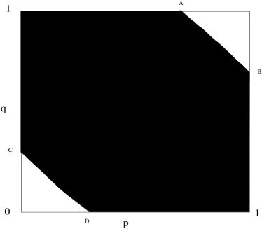
Figure 7: The allowed $(p,q)$ region (shaded area) for the existence of a CPTP mapping between two input mixed states and two output mixed states for the set of parameters: $Y_{0}=4,~{}~{}X=1,~{}~{}R=0.5$ (case 1)). Points $A,B,C,D$ represent, in the order, the intersections of the ellipse (56) with the boundaries $q=1,p=1,p=0$ and $q=0$.

Figure 8: The allowed $(p,q)$ region (shaded area) for the existence of a CPTP mapping between two input mixed states and two output mixed states for the set of parameters: $Y_{0}=4,~{}~{}X=1,~{}~{}R=3.5$ (case 2)). Points $A,B,C,D$ represent, in the order, the intersections of the lines $\hat{q}_{3~{}\pm}$ with the boundaries $p=0,p=1,p=0$ and $p=1$.

Figure 9: The allowed $(p,q)$ region (shaded area) for the existence of a CPTP mapping between two input mixed states and two output mixed states for the set of parameters: $Y_{0}=4,~{}~{}X=1,~{}~{}R=2.5$ (case 3)).

Figure 10: The allowed $(p,q)$ region (shaded area) for the existence of a CPTP mapping between two input mixed states and two output mixed states for the set of parameters: $Y_{0}=4,~{}~{}X=5.5,~{}~{}R=0.52$ (case 4)). The lines (54) intersect with the boundaries $q=1,p=1,p=0$ and $q=0$ at the points $A,D,E,H$, and with ellipse (56) at the points $B,C,F,G$.

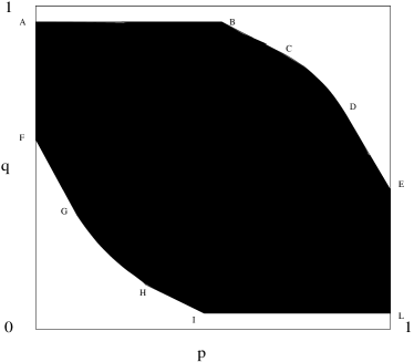
Figure 11: The allowed $(p,q)$ region (shaded area) for the existence of a CPTP mapping between two input mixed states and two output mixed states for the set of parameters: $Y_{0}=4,~{}~{}X=10,~{}~{}R=0.32$ (case 5)). The lines (54) intersect with the the horizontal lines $\hat{q}_{3~{}\pm}$ at the points $B,I$ and with the boundaries $p=0,p=1$ at $F,E$; the horizontal lines $\hat{q}_{3~{}\pm}$ intersect with the boundaries $p=0,p=1$ at $A,L$; the ellipse (56) intersects with the lines (54) at the points $C,D,G,H$.

Figure 12: The allowed $(p,q)$ region (shaded area) for the existence of a CPTP mapping between two input mixed states and two output mixed states for the set of parameters: $Y_{0}=4,~{}~{}X=10,~{}~{}R=0.38$ (case 6)). The lines (54) intersect with the the horizontal lines $\hat{q}_{3~{}\pm}$ at the points $B,E$ and with the boundaries $p=0,p=1$ at $D,C$; the horizontal lines $\hat{q}_{3~{}\pm}$ intersect with the boundaries $p=0,p=1$ at $A,F$.

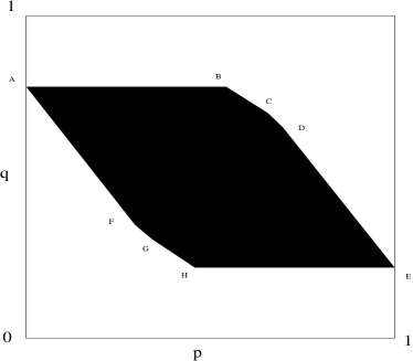
Figure 13: The allowed $(p,q)$ region (shaded area) for the existence of a CPTP mapping between two input mixed states and two output mixed states for the set of parameters: $Y_{0}=4,~{}~{}X=30,~{}~{}R=0.123$ (case 7)). The lines (54) intersect with the the horizontal lines $\hat{q}_{3~{}\pm}$ at the points $B,H$, with the boundaries $p=0,p=1$ at $A,E$, and with the ellipse at the points $C,D,F,G$.