Bohmian Mechanics and Quantum Field Theory

Abstract

We discuss a recently proposed extension of Bohmian mechanics to quantum field theory. For more or less any regularized quantum field theory there is a corresponding theory of particle motion, which in particular ascribes trajectories to the electrons or whatever sort of particles the quantum field theory is about. Corresponding to the nonconservation of the particle number operator in the quantum field theory, the theory describes explicit creation and annihilation events: the world lines for the particles can begin and end.

Despite the uncertainty principle, the predictions of nonrelativistic quantum mechanics permit particles to have precise positions at all times. The simplest theory demonstrating that this is so is Bohmian mechanics Bohm52 ; Ischia ; Stanford ; in this theory the position of a particle cannot be known to macroscopic observers more accurately than the $|\psi|^{2}$ distribution would allow. A frequent complaint about Bohmian mechanics is that, in the words of Steven Weinberg weinlet , “it does not seem possible to extend Bohm’s version of quantum mechanics to theories in which particles can be created and destroyed, which includes all known relativistic quantum theories.”

To remove the grounds of the concern that such an extension may be impossible, we show how, with (more or less) any regularized quantum field theory (QFT), one can associate a particle theory—describing moving particles—that is empirically equivalent to that QFT. In particular, there is a particle theory that recovers all predictions of regularized QED footn1 .

However, we will not attempt to achieve full Lorentz invariance; that would lead to quite a different set of questions, orthogonal to those with which we shall be concerned here. But we note that though the theories we present here require a preferred reference frame, there can be no experiment that would allow an observer to determine which frame is the preferred one, provided the corresponding QFTs are such that their empirical predictions are Lorentz invariant.

The theories we present are based on the work of Bell BellBeables and our own recent results crea1 ; crea2a ; crea2b ; in crea1 we study a simple model QFT, and in crea2a ; crea2b we give a detailed account of the mathematics needed for treating other QFTs. While Bell replaced physical 3-space by a lattice, we describe directly what presumably is the continuum limit of Bell’s model crea2a ; crea2b ; Sudbery ; Vink . Since Bell’s proposal was the first in this direction, we call these models “Bell-type QFTs”. The trajectories we use as the world lines consist of pieces of Bohmian trajectories, or similar ones. A novel element is that the world lines can begin and end. This is essential for describing processes involving particle creation or annihilation, such as, e.g., positron–electron pair creation. Our description of such events is the most naive and natural one: the world line of the particle begins at some space-time point, its creation event, and ends at another (see figure 1). The models thus involve “particle creation” in the literal sense.

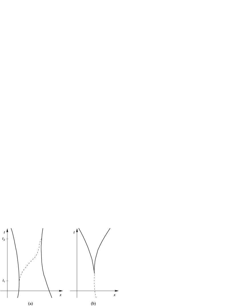
Figure 1: Two patterns of world lines as they may arise from some Bell-type QFT. (a) The world line of a photon (dashed curve) starts at an emission event (at time $t_{1}$) on the world line of an electron (bold curve), and ends at an absorption event (at time $t_{2}$) on the world line of another electron. (b) An electron–positron pair (bold curves) is created at the end point of a photon world line.

The patterns of world lines are reminiscent of Feynman diagrams, and the possible Feynman diagrams correspond to the possible types of world-line patterns. Note, however, that the role of Feynman diagrams is to aid with computing the evolution of the state vector $\Psi$, while the world lines here are supposed to exist in addition to $\Psi$. Unlike Feynman diagrams, which are computational tools not to be confused with actual particle paths, the world-line patterns of our models are to be regarded as describing the possibilities for what might actually happen (in a universe governed by that model).

Whatever the pattern of world lines may look like, it can be described by a time-dependent configuration $Q_{t}=Q(t)$ moving in the configuration space $\mathcal{Q}$ of possible positions for a variable number of particles. In the case of a single particle species, this is the disjoint union of the $n$-particle configuration spaces,

$$\mathcal{Q}=\bigcup_{n=0}^{\infty}\mathcal{Q}^{[n]}\,.$$ (1)

Since the particles are identical, the sector $\mathcal{Q}^{[n]}$ is best defined as $\mathbb{R}^{3n}$ modulo permutations, $\mathbb{R}^{3n}/S_{n}$. For simplicity, we will henceforth pretend that $\mathcal{Q}^{[n]}$ is simply $\mathbb{R}^{3n}$; we discuss $\mathbb{R}^{3n}/S_{n}$ in crea2b . For several particle species, one forms the Cartesian product of several copies of the space (1), one for each species. One obtains in this way a configuration space which is, like (1), a union of sectors $\mathcal{Q}^{[n]}$ where, however, now $n=(n_{1},\ldots,n_{\ell})$ is an $\ell$-tuple of particle numbers for the $\ell$ species of particles. For QED, for example, $\mathcal{Q}$ is the product of three copies of the space (1), corresponding to electrons, positrons, and photons; thus, a configuration specifies the number and positions of all electrons, positrons, and photons foot2 .

Let us explore what $Q(t)$ looks like for a typical world line pattern (see figure 2).

Figure 2: Schematic representation of the configuration space of a variable number of particles. (a)–(d) show the sectors $\mathcal{Q}^{[0]}$ through $\mathcal{Q}^{[3]}$. A configurational history $Q(t)$ jumps to the next higher sector at each creation event, and to the next lower sector at each annihilation event. The history shown corresponds to a world-line pattern like that of figure 1(a).

$Q(t)$ will typically have discontinuities, even if there is nothing discontinuous in the world line pattern (figure 1), because it jumps to a different sector at every creation or annihilation event. Between such events, $Q(t)$ moves smoothly within one sector.

It is helpful to note that the bosonic Fock space can be understood as a space of $L^{2}$ (i.e., square-integrable) functions on $\bigcup_{n}\mathbb{R}^{3n}/S_{n}$. The fermionic Fock space consists of $L^{2}$ functions on $\bigcup_{n}\mathbb{R}^{3n}$ which are anti-symmetric under permutations.

A Bell-type QFT specifies such world-line patterns, or histories in configuration space, by specifying three sorts of “laws of motion”: when to jump, where to jump, and how to move between the jumps. Before we say more on what precisely the laws are, we elucidate one consequence of the laws: if at $t=0$, the configuration $Q(0)$ is chosen at random with probability distribution $|\Psi_{0}|^{2}$, then at any later time $t$, $Q(t)$ has distribution $|\Psi_{t}|^{2}$. This property we call equivariance. The main consequence is that these theories are empirically equivalent to their corresponding QFTs. This conlusion has been explained in detail in DGZ for Bohmian mechanics and the predictions of nonrelativistic quantum mechanics, and the same reasoning applies here. It involves a law of large numbers governing the empirical frequencies in a typical universe, and involves the recognition that the variables that record the outcome of an experiment are ultimately particle positions (orientations of meter pointers, ink marks on paper, etc.).

In a Bell-type QFT, the state of a system is described by the pair $(\Psi_{t},Q_{t})$, where $\Psi_{t}$ is an (arbitrary) vector in the appropriate Fock space and may well involve a superposition of states of different particle numbers. As remarked before, $\Psi_{t}$ can thus be viewed as a function $\Psi_{t}(q)$ on the configuration space $\mathcal{Q}$ of a variable number of particles. (For photons, whose position observable is represented by a positive-operator-valued measure (POVM), $\Psi_{t}$ can be represented by a wavefunction $\Psi_{t}(q)$ satisfying a constraint.) $\Psi_{t}$ evolves according to the appropriate Schrödinger equation

$$i\hbar\frac{d\Psi_{t}}{dt}=H\Psi_{t}\,.$$ (2)

Typically $H=H_{0}+H_{I}$ is the sum of a free Hamiltonian $H_{0}$ and an interaction Hamiltonian $H_{I}$. It is important to appreciate that although there is an actual particle number, defined by $N(t)=\#Q(t):=[\text{number of entries in }Q(t)]$ or $Q(t)\in\mathcal{Q}^{[N(t)]}$, $\Psi$ need not be a number eigenstate (i.e., concentrated on one sector). This is similar to the situation in the usual double-slit experiment, in which the particle passes through only one slit although the wavefunction passes through both. And as with the double-slit experiment, the part of the wavefunction that passes through another sector of $\mathcal{Q}$ (or another slit) may well influence the behavior of $Q(t)$ at a later time.

The laws of motion for $Q_{t}$ depend on $\Psi_{t}$ (and on $H$). The continuous part of the motion is governed by a first-order ordinary differential equation

$$\frac{dQ_{t}}{dt}=v^{\Psi_{t}}(Q_{t})=\mathrm{Re}\,\frac{\Psi_{t}^{*}(Q_{t})\,\big{(}\dot{\hat{q}}\Psi_{t}\big{)}(Q_{t})}{\Psi_{t}^{*}(Q_{t})\,\Psi_{t}(Q_{t})}$$ (3)

$$\mbox{where }\dot{\hat{q}}=\frac{d}{d\tau}\,e^{iH_{0}\tau/\hbar}\,\hat{q}\,e^{-iH_{0}\tau/\hbar}\Big{|}_{\tau=0}=\frac{i}{\hbar}\,\big{[}H_{0},\hat{q}\big{]}$$ (4)

is the time derivative of the $\mathcal{Q}$-valued Heisenberg position operator $\hat{q}$, evolved with $H_{0}$ alone. Since in the absence of global coordinates on $\mathcal{Q}$, the notion of a “$\mathcal{Q}$-valued operator” may be somewhat obscure, one should understand (3) as saying this: for any smooth function $f:\mathcal{Q}\to\mathbb{R}$,

$$\frac{df(Q_{t})}{dt}=\mathrm{Re}\,\frac{\Psi_{t}^{*}(Q_{t})\big{(}\frac{i}{\hbar}[H_{0},\hat{f}]\Psi_{t})(Q_{t})}{\Psi_{t}^{*}(Q_{t})\,\Psi_{t}(Q_{t})}$$ (5)

where $\hat{f}$ is the multiplication operator corresponding to $f$. This expression is of the form $v^{\Psi}\cdot\nabla f(Q_{t})$, as it must be for defining a dynamics for $Q_{t}$, if the free Hamiltonian is a differential operator of up to second order crea2b . The Klein–Gordon operator is not covered by (3) or (5); its treatment will be discussed in future work klein2 . The numerator and denominator of (3) resp. (5) involve, when appropriate, scalar products in spin space. One may view $v$ as a vector field on $\mathcal{Q}$, and thus as consisting of one vector field $v^{[n]}$ on every manifold $\mathcal{Q}^{[n]}$; it is then $v^{[N(t)]}$ that governs the motion of $Q(t)$ in (3).

If $H_{0}$ were the Schrödinger operator $-\sum_{i=1}^{n}\frac{\hbar^{2}}{2m_{i}}\Delta_{i}+V$ of quantum mechanics, formula (3) would yield the velocity proposed by Bohm in Bohm52 ,

$$v^{\Psi}_{i}=\frac{\hbar}{m_{i}}\,\mathrm{Im}\,\frac{\Psi^{*}\nabla_{i}\Psi}{\Psi^{*}\Psi}\,,\>i=1,\ldots,n.$$ (6)

When $H_{0}$ is the “second quantization” of a one-particle Schrödinger operator, (3) amounts to (6), with equal masses, in every sector $\mathcal{Q}^{[n]}$. Similarly, in case $H_{0}$ is the second quantization of the Dirac operator $-ic\hbar{\boldsymbol{\alpha}}\cdot\nabla+\beta mc^{2}$, (3) says a configuration $Q(t)$ (with $N$ particles) moves according to (the $N$-particle version of) the known variant of Bohm’s velocity formula for Dirac wavefunctions BH ,

$$v^{\Psi}=\frac{\Psi^{*}\alpha\Psi}{\Psi^{*}\Psi}\,c\,.$$ (7)

The jumps are stochastic in nature, i.e., they occur at random times and lead to random destinations. In Bell-type QFTs, God does play dice. There are no hidden variables which would fully pre-determine the time and destination of a jump. (Note also that a deterministic jump law that prescribes the time and destination of the jump as a (smooth) function of the initial configuration would lack sufficient randomness to be compatible with equivariance, since after a jump from a sector with dimension $d^{\prime}$ to a sector with dimension $d>d^{\prime}$ the configuration would have to belong, at any specific time, to a $d^{\prime}$-dimensional submanifold.)

The probability of jumping, within the next $dt$ seconds, to the volume $dq$ in $\mathcal{Q}$, is $\sigma^{\Psi}(dq|Q_{t})\,dt$ with

$$\sigma^{\Psi}(dq|q^{\prime})=\frac{2}{\hbar}\frac{[\mathrm{Im}\,\Psi^{*}(q)\,\langle q|H_{I}|q^{\prime}\rangle\,\Psi(q^{\prime})]^{+}}{\Psi^{*}(q^{\prime})\,\Psi(q^{\prime})}\,dq\,,$$ (8)

where $x^{+}=\max(x,0)$ means the positive part of $x\in\mathbb{R}$. Thus the jump rate $\sigma^{\Psi}$ depends on the present configuration $Q_{t}$, on the state vector $\Psi_{t}$, which has a “guiding” role similar to that in Bohm’s velocity law (6), and of course on the overall setup of the QFT as encoded in the interaction Hamiltonian $H_{I}$. In crea1 , we spelled out in detail a simple example of a Bell-type QFT.

Together, (3) and (8) define a Markov process on $\mathcal{Q}$. The “free” part of this process, defined by (3), can also be regarded as arising as follows: if $H_{0}$ is as usual the “second quantization” of a 1-particle Hamiltonian $h$, one can construct the dynamics corresponding to $H_{0}$ from a given 1-particle dynamics corresponding to $h$ (be it deterministic or stochastic) by an algorithm that one may call the “second quantization” of a Markov process crea2b . Moreover, this algorithm can still be used when formula (3) fails to define a dynamics (in particular when $H_{0}$ is the second quantized Klein–Gordon operator).

We now discuss the role of field operators (operator-valued fields on space-time) in a theory of particles. Almost by definition, it would seem that QFT concerns fields, and not particles. But there is less to this than might be expected. The field operators do not function as observables in QFT. It is far from clear how to actually “observe” them, and even if this could somehow, in some sense, be done, it is important to bear in mind that the standard predictions of QFT are grounded in the particle representation, not the field representation: Experiments in high energy physics are scattering experiments, in which what is observed is the asymptotic motion of the outgoing particles. Moreover, for Fermi fields—the matter fields—the field as a whole (at a given time) could not possibly be observable, since Fermi fields anti-commute, rather than commute, at space-like separation. We note, though, that a theory in which $\Psi_{t}$ guides an actual field can be devised, at least formally Bohm52 .

The role of the field operators is to provide a connection, the only connection in fact, between space-time and the abstract Hilbert space containing the quantum states $|\Psi\rangle$, which are usually regarded not as functions but as abstract vectors. For our purpose, what is crucial are the following facts that we shall explain presently: (i) the field operators naturally correspond to the spatial structure provided by a projection-valued (PV) measure on configuration space $\mathcal{Q}$, and (ii) the process we have defined in this paper can be efficiently expressed in terms of a PV measure.

Consider a PV measure ${P}$ on $\mathcal{Q}$ acting on $\mathcal{H}$: For $B\subseteq\mathcal{Q}$, ${P}(B)$ means the projection to the space of states localized in $B$. All our formulas above can be formulated in terms of ${P}$ and $|\Psi\rangle$: (5) becomes

$$\frac{df(Q_{t})}{dt}=\mathrm{Re}\,\frac{\langle\Psi|{P}(dq)\frac{i}{\hbar}[H_{0},\hat{f}]|\Psi\rangle}{\langle\Psi|{P}(dq)|\Psi\rangle}\Big{|}_{q=Q_{t}}$$ (9)

$$\mbox{with }\hat{f}=\int\limits_{q\in\mathcal{Q}}f(q)\,{P}(dq)\,,$$ (10)

for any smooth function $f:\mathcal{Q}\to\mathbb{R}$, and (8) becomes

$$\sigma^{\Psi}(dq|q^{\prime})=\frac{2}{\hbar}\frac{[\mathrm{Im}\,\langle\Psi|{P}(dq)H_{I}{P}(dq^{\prime})|\Psi\rangle]^{+}}{\langle\Psi|{P}(dq^{\prime})|\Psi\rangle}.$$ (11)

Note that $\langle\Psi|{P}(dq)|\Psi\rangle$ is the probability distribution analogous to $|\Psi(q)|^{2}dq$.

We now turn to (i): how we obtain the PV measure ${P}$ from the field operators. For the configuration space $\mathcal{Q}=\bigcup_{n}\mathbb{R}^{3n}/S_{n}$ of a variable number of identical particles, a configuration can be specified by giving the number of particles $n(R)$ in every region $R\subseteq\mathbb{R}^{3}$. A PV measure ${P}$ on $\mathcal{Q}$ is mathematically equivalent to a family of number operators: an additive operator-valued set function $N(R)$, $R\subseteq\mathbb{R}^{3}$, such that the $N(R)$ commute pairwise and have spectra in the nonnegative integers. Indeed, ${P}$ is the joint spectral decomposition of the $N(R)$ crea2b . And the easiest way to obtain such a family of number operators is by setting

$$N(R)=\int_{R}\phi^{*}({\boldsymbol{x}})\,\phi({\boldsymbol{x}})\,d^{3}{\boldsymbol{x}}\,,$$

exploiting the canonical commutation or anti-commutation relations for the field operators $\phi({\boldsymbol{x}})$. These observations suggest that field operators are just what the doctor ordered for the efficient construction of a theory describing the creation, motion, and annihilation of particles.

(It is only the positive-energy one-particle states that are used for constructing the Fock space $\mathcal{H}$, so that $\mathcal{H}$ is really a subspace of a larger Hilbert space $\mathcal{H}_{0}$ which contains also unphysical states (with contributions from one-particle states of negative energy). Since position operators may fail to map positive energy states into positive energy states, the PV measure ${P}$ is typically defined on $\mathcal{H}_{0}$ but not on $\mathcal{H}$, in which case (9) and (11) have to be read as applying in $\mathcal{H}_{0}$. While $H_{0}$ is defined on $\mathcal{H}_{0}$, $H_{I}$ is usually not and needs to be “filled up with zeroes”, i.e. replaced by $P^{\prime}H_{I}P^{\prime}$ where $P^{\prime}$ is the projection $\mathcal{H}_{0}\to\mathcal{H}$.)

To sum up, we have shown how the realist view which Bohmian mechanics provides for the realm of nonrelativistic quantum mechanics can be extended to QFT, including creation and annihilation of particles. Those who find the all too widespread positivistic attitude in quantum theory unsatisfactory may find these ideas helpful. But even those who think that Copenhagen quantum theory is just fine may find it interesting to see how the particle picture, ubiquitous in the pictorial lingo and heuristic intuition of QFT, can be made consistent, internally and with the observable facts of QFT, by introducing suitable laws of motion.

References

- (1) D. Bohm, Phys. Rev. 85, 166-179 (1952). D. Bohm, Phys. Rev. 85, 180-193 (1952).
- (2) D. Dürr, in J. Bricmont et al. (eds.): Chance in Physics: Foundations and Perspectives (Berlin: Springer-Verlag 2001).
- (3) S. Goldstein, “Bohmian Mechanics” (2001), in Stanford Encyclopedia of Philosophy (Winter 2002 Edition), E.N. Zalta (ed.), http://plato.stanford.edu/archives/ win2002/entries/qm-bohm/.
- (4) S. Weinberg (private communication).
- (5) One may worry that such a particle theory, in which particles always have actual positions but have no additional actual discrete degrees of freedom corresponding for example to spin, cannot do justice to QFT, for which spin and other discrete degrees of freedom are often regarded as playing a crucial role. However, additional actual discrete degrees of freedom are entirely unnecessary: as Bell has shown in 1966 , the straightforward extension of Bohmian mechanics to spinor-valued wavefunctions, which we use here, accounts for all phenomena involving spin.
- (6) J. S. Bell, Rev. Mod. Phys. 38, 447–452 (1966).
- (7) J. S. Bell, Phys. Rep. 137, 49-54 (1986).
- (8) D. Dürr, S. Goldstein, R. Tumulka, and N. Zanghì, J. Phys. A: Math. Gen. 36, 4143-4149 (2003).
- (9) D. Dürr, S. Goldstein, R. Tumulka, and N. Zanghì, quant-ph/0303056 [Commun. Math. Phys. (to be published)].
- (10) D. Dürr, S. Goldstein, R. Tumulka, and N. Zanghì, quant-ph/0407116.
- (11) A. Sudbery, J. Phys. A: Math. Gen. 20, 1743-1750 (1987).
- (12) J. C. Vink, Phys. Rev. A 48, 1808-1818 (1993).
- (13) The choice of for a given QFT, such as QED, is however not unique. For instance, it is possible to devise a version of the theory in which the configuration variable represents only the configuration of the fermions BellBeables . We have argued in crea1 that it is more natural to include photons among the particles, represented in .
- (14) D. Dürr, S. Goldstein, and N. Zanghì, J. Statist. Phys. 67, 843-907 (1992).
- (15) D. Dürr, S. Goldstein, R. Tumulka, and N. Zanghì, “Trajectories From Klein–Gordon Functions”, in preparation.
- (16) D. Bohm and B. J. Hiley, The Undivided Universe: An Ontological Interpretation of Quantum Theory (London: Routledge, Chapman and Hall 1993), p. 274.