Berry phase for a spin 1/2 in a classical fluctuating field

Abstract

The effect of fluctuations in the classical control parameters on the Berry phase of a spin 1/2 interacting with a adiabatically cyclically varying magnetic field is analyzed. It is explicitly shown that in the adiabatic limit dephasing is due to fluctuations of the dynamical phase.

Berry phase Berry and related geometrical phases shapere ; zee have received renewed interest in recent years due to several proposal for their use in the implementation of quantum computing gates ws ; Jones ; Zanardi ; falci00 ; ekert ; cleve ; barenco ; wilhelm ; zoller ; keiji ; ekertgqc . Such interest is motivated by the belief that geometric quantum gates should exhibit an intrinsic fault tolerance in the presence of external noise. Such belief is based on the heuristic argument that being Berry phases geometrical in their nature, i.e. proportional to the area spanned in parameter space, any fluctuating perturbation of zero average should indeed average out. Although this argument seems convincing to the best of our knowledge it has not been quantitatively probed so far. In particular although several papers blais ; spiller ; gefen have investigated aspects of Berry phases in the presence of quantum external noise we are not aware of any in which the effect of classical noise in a simple model of qubit, namely a spin 1/2 interacting with an external classical field with a fluctuating component has been analyzed. This is precisely the aim of this paper. For such system the effects of classical fluctuations in the control parameter on both geometric and dynamic phases is studied and their impact on dephasing analyzed. Our system consists of a spin 1/2 in the presence of an external static magnetic field, whose Hamiltonian, in appropriate units, takes the form

$$H(t)=\frac{1}{2}{\bf B}(t)\cdot\vec{\sigma}$$ (1)

where $\vec{\sigma}=(\sigma_{x},\sigma_{y},\sigma_{z})$, $\sigma_{i}$ are the Pauli operators and ${\bf B}(t)=B_{0}(t)\hat{n}(t)$ with the unit vector $\hat{n}=(\sin\vartheta\cos\varphi,\sin\vartheta\sin\varphi,\cos\vartheta)$. The classical field ${\bf B}(t)$ acts as an external control parameter, as its direction and magnitude can be experimentally changed. When varied adiabatically the instantaneous energy eigenstates follow the direction of $\hat{n}$ and therefore can be expressed as

$$|\uparrow_{n}\rangle = e^{-i\varphi/2}\cos\frac{\vartheta}{2}|\uparrow\rangle+e^{i\varphi/2}\sin\frac{\vartheta}{2}|\downarrow\rangle$$

$$|\downarrow_{n}\rangle = e^{-i\varphi/2}\sin\frac{\vartheta}{2}|\uparrow\rangle-e^{i\varphi/2}\cos\frac{\vartheta}{2}|\downarrow\rangle$$ (2)

where $|\uparrow\rangle,|\downarrow\rangle$ are the eigenstates of the $\sigma_{z}$ operator.

When the time evolution is cyclic i.e. when after a time $T$ we have ${\bf B}(T)={\bf B}(0)$ the energy eigenstates acquire a phase factor which contains a geometric correction to the dynamic phase:

$$|\uparrow_{n(T)}\rangle=e^{i\delta}e^{i\gamma_{B}}|\uparrow_{n(0)}\rangle$$ (3)

where the dynamic phase $\delta=\int_{0}^{T}B_{0}(t)dt$ and the Berry phase can be expressed in term of the so called Berry connection ${\bf A}^{\uparrow}=i\langle\uparrow_{n}|\nabla_{\lambda}|\uparrow_{n}\rangle$ as $\gamma_{B}=\oint{\bf A}^{\uparrow}\cdot d\vec{\lambda}$ where $\vec{\lambda}$ is the set of control parameters. In our specific example $\vec{\lambda}=(\vartheta,\varphi)$. An analogous expression holds for ${\bf A}^{\downarrow}$, relative to the $|\downarrow_{n}\rangle$ state. It is straightforward to calculate the components of ${\bf A}$:

$$A_{\varphi}^{\uparrow} = -A_{\varphi}^{\downarrow}=i\langle\uparrow_{n}|\partial/\partial\varphi|\uparrow_{n}\rangle=\frac{1}{2}\cos\vartheta$$ (4)

$$A_{\vartheta}^{\uparrow} = -A_{\vartheta}^{\downarrow}=i\langle\uparrow_{n}|\partial/\partial\vartheta|\uparrow_{n}\rangle=0$$ (5)

It is important to note that while the eigenenergies depend on $B_{0}(t)$ the eigenstates depend only on $\hat{n}(t)$. As a consequence the Berry phase depends only on $\vartheta,\varphi$. A standard example is a slow precession of ${\bf B}$ at an angle $\vartheta$ around the $z$ axis with angular velocity $\omega=2\pi/T\ll B_{0}$. A straightforward calculation shows that

$$\gamma_{\uparrow}=-\gamma_{\downarrow}=\int_{0}^{2\pi}A_{\varphi}^{\uparrow}d\varphi=\pi\cos\vartheta$$ (6)

Note that the the Berry phase is proportional to the solid angle subtended by ${\bf B}$ with respect to the degeneracy ${\bf B}=0$

We are now in the position to extend our analysis to the case in which the magnetic field contains a fluctuating component. In this case Hamiltonian (1) is modified as follows

$$H(t)=\frac{1}{2}\mathbf{B}_{T}\cdot\vec{\sigma}=\frac{1}{2}(\mathbf{B}(t)+\mathbf{K}(t))\cdot\vec{\sigma}$$ (7)

where we have divided the total magnetic field $\mathbf{B}_{T}$ into an average component $\mathbf{B}$ experimentally under our control and a fluctuating field $\mathbf{K}$. We will analyze the case in which $\mathbf{B}$ is a field of constant amplitude which undergoes a cyclic evolution while the components of $\mathbf{K}$ are random processes with zero average and small amplitude compared to $\mathbf{B}$, in order to consider lowest order corrections. Finally we will assume that the fluctuations are characterized by timescales such that the adiabatic approximation holds. We will show that this is not an unphysical restriction.

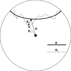
Figure 1: Generic path of the total magnetic field $\mathbf{B}_{T}$. The field $\mathbf{B}$ is under experimental control and undergoes a cyclic evolution while $\mathbf{K}$ is a small random fluctuating field. Note that in general $\mathbf{K}$ fluctuates both in the direction parallel and perpendicular to $\mathbf{B}$.

Corrections to (6) have a twofold origin as the fluctuating field $\bf{K}$ modifies both the connection $\bf{A}$ and the path. To first order correction the connection is

$$A_{\varphi}(\vartheta) \cong A_{\varphi}(\vartheta_{0})+\frac{\partial A_{\varphi}}{\partial\vartheta}\delta\vartheta=$$ (8)

$$=\frac{1}{2}\left(\cos\vartheta_{0}-\delta\vartheta\sin\vartheta_{0}\right)$$ (9)

where $\vartheta_{0}$ is the polar angle of the average field $\bf{B}$ while $\delta\vartheta$ is the fluctuation of the polar angle due to the fluctuating field $\bf{K}$. In order to analyze the corrections to the path, with no loss of generality, we again consider the case of a slow precession of $\bf{B}$ around the $\hat{z}$ axis. In the presence of $\bf{K}$ the line element $d\vec{\lambda}$ will have also a component perpendicular to the orbit of $\bf{B}$ . However as the connection $\bf{A}$ has zero component in the $\vartheta$ direction we can restrict our attention to the $\varphi$ component of $d\vec{\lambda}$. To this end we write

$$d\lambda=\dot{\varphi}dt\cong(\dot{\varphi}_{0}+\delta\dot{\varphi})dt$$ (10)

In (10) $\dot{\varphi}_{0}$ is the average angular velocity. In our case $\dot{\varphi}_{0}=2\pi/T$ while $\delta\dot{\varphi}$ is the first order correction due to $\mathbf{K}$: in particular when $\mathbf{K}$ fluctuates in the same direction of $\mathbf{\dot{B}}$ the precession speed increases while it decreases in the case of fluctuation in the opposite direction. Note that fluctuations in the path contain only corrections in $\varphi$ while fluctuations in the connection depend only on $\vartheta$. This is independent from any approximation but is due to the structure of the connection.

We can now express the Berry phase in the presence of noise as

$$\gamma_{B} =\int_{0}^{T}(A_{\varphi}(\vartheta_{0})+\delta A_{\varphi})(\dot{\varphi}_{0}+\delta\dot{\varphi})dt$$ (11)

$$\cong\gamma_{B}^{0}+\frac{2\pi}{T}\int_{0}^{T}\delta A_{\varphi}dt+A_{\varphi}(\vartheta_{0})\int_{0}^{T}\delta\dot{\varphi}dt$$

$$=\gamma_{B}^{0}-\frac{\pi}{T}\int_{0}^{T}\sin\vartheta_{0}\delta\vartheta dt+A_{\varphi}(\vartheta_{0})\delta\varphi(T)$$

where the average Berry phase $\gamma_{B}^{0}$ coincides with $\gamma_{B}$ in the absence of noise and it has been assumed $\delta\varphi(0)=0$. The last term in (11) is a non-cyclic contribution which appears when, due to the presence of $\mathbf{K}$, $\mathbf{B}_{T}$ does not return to its original. In this case, instead of the geometrical phase definition given by Berry, which assumes that the Hamiltonian is periodic, we have to use the definition by Samuel and Bhandari SamBha88 about non cyclic evolution. If this is done the third term does not appear and eq.(11) becomes:

$$\gamma_{B}=\gamma_{B}^{0}-\frac{\pi}{T}\int_{0}^{T}\sin\vartheta_{0}\delta\vartheta dt$$ (12)

In order to proceed a physical model for the noise is needed, in other words a stochastic process for $\mathbf{K}$ must be assigned. Given the probability distribution for the field it is straightforward to calculate the distribution for the Berry phase.

As a first step we express the trigonometric functions appearing in (12) in terms of the fluctuating field components $K_{i}$. This will be useful in calculating the probability distribution for $\gamma_{B}$. Let $\vartheta_{0}$ , $\varphi_{0}$ be the polar angles of $\mathbf{B}$; $\vartheta$ , $\varphi$ those of $\mathbf{B_{T}}$; and $\delta\vartheta$ , $\delta\varphi$ the first order differences between the polar angles of the two fields. Moreover let $B=|\mathbf{B}|$ be the modulus of $\mathbf{B}$. If we expand in Taylor series $\cos\vartheta$ we obtain:

$$\cos(\vartheta_{0}+\delta\vartheta)\cong\cos\vartheta_{0}-\delta\vartheta\sin\vartheta_{0}=\frac{B_{3}}{B}+\frac{K_{3}}{B}-\frac{B_{3}}{B^{3}}\mathbf{B}\cdot\mathbf{K}$$

and therefore

$$-\delta\vartheta\sin\vartheta_{0}=\frac{K_{3}}{B}-\frac{B_{3}}{B^{3}}\mathbf{B}\cdot\mathbf{K}$$ (13)

Substituting equation (13) in (12) we find:

$$\gamma_{B}=\gamma_{B}^{0}+\frac{\pi}{T}\int_{0}^{T}\left[\frac{K_{3}}{B}-\frac{B_{3}}{B^{3}}\mathbf{B}\cdot\mathbf{K}\right]dt$$ (14)

From this expression it is possible to find the probability distribution for $\gamma_{B}$, once that for $K_{i}$ is known.

We will assume that the fluctuating field $K_{i}$ is a Ornstein-Uhlenbeck process, i.e it is gaussian, stationary and markovian with a lorentzian spectrum whose bandwidth $\Gamma_{i}$ we assume to be much less than the Bohr frequency of our energy eigenstates. However while we must have $\omega\ll B$ and $\Gamma_{i}\ll B$ we have no restriction on the relative value of $\omega$ vs $\Gamma_{i}$. In order to allow for the possibility of anisotropic noise we assume that $K_{3}$ has variance $\sigma_{3}$ and bandwidth $\Gamma_{3}$ while $K_{1}$ and $K_{2}$ have $\sigma_{12}$ and $\Gamma_{12}$.

With these assumption we found that the distribution for $\gamma_{B}$ is a gaussian whose mean value, as said before, is the noiseless Berry phase and whose variance is

$$\sigma^{2}_{\gamma}=2\sigma_{12}^{2}\left(\frac{\pi\cos\vartheta_{0}\sin\vartheta_{0}}{TB}\right)^{2}\left[\frac{(e^{-\Gamma T}-1)(\Gamma^{2}-\omega^{2})}{(\Gamma^{2}+\omega^{2})^{2}}+\frac{\Gamma T}{\Gamma^{2}+\omega^{2}}\right]+2\sigma_{3}^{2}\left(\frac{\pi\sin^{2}\vartheta_{0}}{TB}\right)^{2}\left[\frac{\Gamma T-1+e^{-\Gamma T}}{\Gamma^{2}}\right]$$ (15)

This expression has an interesting limiting value when $\Gamma_{i}\ll\omega$ and $\Gamma_{i}\gg\omega$. To first order in $\Gamma T$:

$$\!\sigma^{2}_{\gamma}\!=4\sigma_{12}^{2}\!\!\left(\!\!\frac{\pi\!\cos\vartheta_{0}\!\sin\vartheta_{0}}{B}\!\!\right)^{2}\!\!\frac{\Gamma_{12}T}{(2\pi)^{2}}+2\sigma_{3}^{2}\!\!\left(\!\frac{\!\pi\sin^{2}\!\vartheta_{0}}{B}\!\!\right)^{2}\!\!\!\left(\!\frac{1}{2}-\frac{\Gamma_{3}T}{6}\!\right)$$ (16)

We see that the leading term is $\sigma_{3}^{2}\left(\frac{\pi\sin^{2}\vartheta_{0}}{B}\right)^{2}$ which tends to zero for little $\vartheta_{0}$.

When $T\gg\Gamma^{-1}$ the fluctuating field has time enough to make many uncorrelated oscillations during the cyclic evolution. In this case the effect of the fluctuations averages out and in the limit $(\Gamma T)^{-1}\to 0$ do not give contribution to the variance which tends to zero:

$$\!\sigma^{2}_{\gamma}=2\sigma_{12}^{2}\!\left(\!\frac{\pi\cos\vartheta_{0}\sin\vartheta_{0}}{B}\!\right)^{2}\!\!\frac{1}{\Gamma_{12}T}+2\sigma_{3}^{2}\left(\frac{\pi\sin^{2}\vartheta_{0}}{B}\right)^{2}\!\!\frac{1}{\Gamma_{3}T}$$ (17)

This is to be compared to the dynamical phase which grows linearly in $T$. This different behavior is due to the fact that while Berry phase corrections are proportional to $1/T\int Kdt$, corrections to the dynamical phase are proportional to $\int Kdt$. For a OU process the variance of the integral grows linearly for times long compared to the autocorrelation time of the field. This is analogous to the variance of the position of a brownian particle.

Until now we concentrated only in the geometrical phase. However during an adiabatic cyclic evolution the eigenstates acquire both the dynamical and geometrical phase. It is known that the dynamical phase $\delta$ is proportional to the modulus of the magnetic field. This means that the dynamical phase becomes a stochastic processes like the Berry phase. We can write $\delta$ in terms of the fields $\vec{B}$ and $\vec{K}$ as we did for the geometrical phase:

$$\delta=\delta_{0}+\int_{0}^{T}\frac{\vec{B}\cdot\vec{K}}{B}dt$$ (18)

where $\delta_{0}=BT$ Note that expression (18) is similar to (14) for Berry phase. The difference is that while $\gamma_{B}$ comes from an integral in parameter space, $\delta$ from an integral in the time domain. For instance this means that if we double time $T$, $\gamma_{B}$ scales with $T^{-1}$ while the domain of integration of $\delta$ doubles. As we will see this is crucial for the different role of the two phases in dephasing.

Following the same steps as for the Berry phase it is possible to demonstrate that $\delta$ is a stochastic processes with a gaussian distribution. Now we analyze the effect of noise on the coherence of a system, in other words dephasing. Suppose we prepare the system in a state which is a superposition of the two eigenstate of the Hamiltonian:

$$\left|\psi\right\rangle=a\left|\uparrow\right\rangle+b\left|\downarrow\right\rangle$$ (19)

After a slowly cyclic evolution the eigenstates have acquired both the dynamical and geometrical phases and the final state is:

$$\left|\psi^{\prime}\right\rangle=ae^{i\alpha}\left|\uparrow\right\rangle+be^{-i\alpha}\left|\downarrow\right\rangle$$ (20)

where $\alpha=\gamma_{B}+\delta$ is the total phase. In the presence of noise this phase is a random variable with a gaussian distribution $P(\alpha)$ then actually the system at the end of the evolution is in a mixed state.

It can be described by the density operator which is given by the expression:

$$\rho=\int\left|\psi^{\prime}\right\rangle\left\langle\psi^{\prime}\right|P(\alpha)d\alpha$$ (21)

We want to stress that $P(\alpha)\neq P(\gamma_{B})P(\delta)$, i.e. dynamical and geometrical phases are not independent processes because both depend on $\vec{K}$.

If we insert eq.(20) in the definition of $\rho$ we find that the population are unchanged while the coherence are shrunk by a factor $\exp(-2\sigma^{2}_{\alpha})$. In terms of the Bloch vector, this means that the $z$ component is unchanged while the component parallel to the $xy$ is reduced. This is what is called dephasing because the relative phase in a superposition is undefined.

In order to do not lose in generality and to compare the dynamical and geometrical phase we have studied the two case together. We have found the probability distribution $P(\alpha)$ for $\alpha$ which has mean value $\langle\alpha\rangle=\langle\gamma_{B}\rangle+\langle\delta\rangle$ and variance:

$$\sigma_{\alpha}^{2} =2\frac{\sigma_{12}^{2}}{B^{2}}\left(-\frac{\pi\cos\vartheta_{0}\sin\vartheta_{0}}{T}+B\sin\vartheta_{0}\right)^{2}\times$$ (22)

$$\left[\frac{(e^{-\Gamma_{12}T}-1)(\Gamma_{12}^{2}-\omega^{2})}{(\Gamma_{12}^{2}+\omega^{2})^{2}}+\frac{\Gamma_{12}T}{\Gamma_{12}^{2}+\omega^{2}}\right]$$

$$+2\frac{\sigma_{3}^{2}}{B^{2}}\left(\frac{\pi\sin^{2}\vartheta_{0}}{T}+B\cos\vartheta_{0}\right)^{2}\left[\frac{\Gamma_{3}T-1+e^{-\Gamma_{3}T}}{\Gamma_{3}^{2}}\right]$$

In eq. (22) $\sigma_{\alpha}^{2}$ is the sum of two terms one coming from fluctuation in z direction and one in the xy plane. Each of these terms contains a factor in round brackets in which we recognize a geometrical term proportional to $1/T$, as we found in (15) and a dynamical one proportional to the Bohr frequency. Now because of the adiabaticity condition we have that the first is much less than the second. As a consequence the main contribution to dephasing has dynamical rather than geometrical origin. This does do not mean of course that in a system in which Berry phase emerges dephasing is less than in a system in which it does not. What we have demonstrated is that fluctuations in Berry phase do not contribute considerably to dephasing.

Another relevant aspect to stress is that our calculation was performed under the assumptions of a constant circular precession, however our results are independent of the specific path executed by the magnetic field as long as the adiabatic approximation is valid.

It is worth noting that dephasing is not the only decoherence source in our system. The Bloch vector in fact does not return to its initial position since the magnetic field does not. To calculate the correct Bloch vector we have to average the final positions. However the contributions from this effect are proportional to $(K_{i}/B)^{2}$ and so we can neglect this effect at our level of approximation.

In this paper we have calculated the distribution of Berry phase in the presence of classical noise. Assuming a OU process for noise we found that under the assumption of small fluctuation Berry phase is a gaussian variable. We have calculated its mean value and the variance and we found that the variance diminishes as $1/T$. This is to be compared to the variance of the dynamical phase which grows linearly with $T$. This shows that adiabaticity and the geometrical aspects of Berry phase reduce fluctuations. This is what was expected but never demonstrated. Another aspect that makes Berry phase more robust than dynamical phase is that of dephasing. We showed that geometrical dephasing is much less than the dynamical one. This is due mainly to adiabaticity. This means that probably quantum gates based upon geometrical phase are more resistant. We would like to point out that after we submitted our manuscript a paper has appeared carollo in which the noise is treated fully quantum mechanically and similar conclusions have been drawn (but in a completely different setting) about the invariant of the geometric phase. These two results together complement each other.

References

- (1) M.V. Berry, Proc. Roy. Soc. A 392, 47 (1984)reprinted in
- (2) Geometric phases in physics, A. Shapere and F. Wilczek, Eds. World Scientific, (Singapore, 1989).
- (3) F. Wilczek and A.Zee, Phys. Rev. Lett. 52, 2111 (1999).
- (4) Quantum computation and quantum information theory C.Macchiavello, G.M.Palma & A.Zeilinger Ed.s, World Scientific, (Singapore, 2000).
- (5) J. Jones, V. Vedral, A.K. Ekert, C. Castagnoli, Nature, 403, 869 (2000).
- (6) P. Zanardi and M. Rasetti, Phys. Lett. A, 264, 94 (1999).
- (7) G. Falci, R. Fazio, G.M. Palma, J. Siewert, and V. Vedral, Nature 403, 869 (2000).
- (8) M.-M Duan, I. Cirac and P. Zoller, Science 292, 1695 (2001).
- (9) A. Ekert and R. Jozsa, Rev. Mod. Phys. 68, 733 (1996).
- (10) R. Cleve, A. Ekert, L. Henderson, C. Macchiavello, M. Mosca On quantum algorithms Complexity Vol.4, No.1, pp.33-42 (1998). quant-phys/9903061 Reprinted in reference ws .
- (11) D. Deutsch, A. Barenco, A. Ekert, Proc. R. Soc. London A 449, 669 (1995).
- (12) X.-B. Wang, K. Matsumoto, J. Phys. A: Math. Gen. 34, L631 (2001) and Phys.Rev.Lett. 87, 097901 (2001).
- (13) A. Ekert , M. Ericsson, P. Hayden, H. Inamori, J. A. Jones, D. K. L. Oi and V. Vedral, J. Mod. Opt.47, 2501 (2000).
- (14) F.K. Wilhelm and J.E. Mooij, preprint 2001.
- (15) A. Blais, A.-M.S. Tremblay, Phys.Rev. A 67, 012308 (2003).
- (16) A. Nazir, T. P. Spiller, and W. J. Munro, Phys. Rev. A 65, 042303 (2002).
- (17) R.S. Whitney and Y. Gefen, Proceedings of XXXVIth Rencontres de Moriond (Jan 2001) Electronic correlations: from Meso- to Nano-physics; cond-mat/0107359.
- (18) J. Samuel and R. Bhandari, Phys. Rev. Lett. 60 2339 (1988)
- (19) A. Carollo, I. Fuentes-Guridi, M. Fran a Santos, and V. Vedral, Phys. Rev. Lett.90, 160402, (2003)