Linear optics substituting scheme for multi-mode operations

Abstract

We propose a scheme allowing a conditional implementation of suitably truncated general single- or multi-mode operators acting on states of traveling optical signal modes. The scheme solely relies on single-photon and coherent states and applies beam splitters and zero- and single-photon detections. The signal flow of the setup resembles that of a multi-mode quantum teleportation scheme thus allowing the individual signal modes to be spatially separated from each other. Some examples such as the realization of cross-Kerr nonlinearities, multi-mode mirrors, and the preparation of multi-photon entangled states are considered.

I Introduction

A general problem in quantum optics is the implementation of a defined single- or multi-mode operator by some physical scheme since many efforts amount to the realization of a desired quantum state transformation of an unknown or control of a known signal quantum state Lloyd (1994, 1995); Lloyd and Braunstein (1999); Lloyd and Slotine (2000); Lloyd (2000); Lloyd and Viola (2001); Vogel et al. (1993); Harel and Akulin (1999); Kurizki et al. (2000); Akulin et al. (2001); Solomon and Schirmer (2002); Schirmer et al. (2002a, b); Drobný et al. (1998, 1999); Hladký et al. (2000). Here, we limit attention to a physical system consisting of a number of traveling light pulses described by non-monochromatic signal modes. We assume that the spatial pulse length is large compared to the wavelength of the radiation, so that we deal with quasi-monochromatic pulses corresponding to quasi-orthogonal modes.

A difficulty is that at present, only a limited set of basic operations can be implemented directly. Composite operations therefore have to be constructed from elementary ones which are simple enough to allow their direct realization. Examples of such basic operations are the preparation of coherent (i.e., Glauber) states by single-mode lasers, or single-photon states by parametric down converters, furthermore parametric interactions as realized by beam splitters, three-wave mixers, and Kerr-nonlinearities, and the discrimination between presence and absence of photons by means of binary 0-1-photodetectors such as Avalanche photodiodes. A simple combination of these techniques allows further manipulations such as parametric amplification, coherent displacement, or the preparation and detection of photon number (i.e., Fock) states Kok and Braunstein (2001).

To give an example, the signal pulse may be sent through a medium applied in the parametric approximation, i.e., the medium realizes a weak coupling between the signal modes and a number of auxiliary modes prepared in strong coherent states. Since within classical optics, $n$th-order interactions are described as a $n$th-order deviation from linearity of the polarization induced in a medium by an electric field, the interaction strength is expected to decline rapidly with increasing order. Strong fields are therefore required for their observation. In contrast, setups discussed within quantum optics and quantum information processing often operate with superpositions of low-excited Fock states while the coherent amplitudes in the auxiliary modes cannot be increased unlimited to achieve a desired interaction strength of the reduced signal operation. This greatly limits the order of the nonlinearity applicable and with it the variety of unitary transformations that can be realized by a given medium. Desirable are therefore substituting schemes for such nonlinear interactions Fiurášek and Peřina (2000); Wallentowitz and Vogel (1997). In particular, one may apply the nonlinearity hidden in the quantum measurement process and to use merely passive optical elements such as beam splitters Reck et al. (1994) and photodetectors while relying on simple auxiliary preparations such as coherent and single-photon states Knill et al. (2001). A local measurement performed on a spatially extended quantum system affects the reduced state at the other locations. By repeated measurements and postselection of desired detection events, this back-action caused by a measurement can then be used to perform well-defined manipulations, including state preparations Steuernagel (1997); Paris (2000); Ş. K. Özdemir et al. (2001); Zou et al. (2002a, b, c); Lee et al. (2002); Fiurášek (2002), quantum logic operations Koashi et al. (2001); Ralph et al. (2001); Pittman et al. (2001); Zou et al. (2002d); Ralph et al. (2002); Zou et al. (2002e), state purifications Pan et al. (2001), quantum error corrections Gottesman et al. (2001), and state detections Dušek (2001); Calsamiglia (2002). The simplest basic operations one may think of are the application of the mode operators $\hat{a}$ and $\hat{a}^{\dagger}$, i.e., photon subtraction and addition Dakna et al. (1998); Calsamiglia et al. (2001). With regard to compositions, it is necessary to limit operation to a suitably chosen finite-dimensional subspace of the system’s Hilbert space, cf., e.g., Gottesman et al. (2001), since only a finite number of parameters can be controlled.

The aim of this paper is to investigate a theoretical possibility of implementing a desired single- or multi-mode operation $\hat{Y}$ on the quantum state $\hat{\varrho}$ of a traveling optical signal. The scheme solely relies on beam splitters as well as zero- and single-photon detections. In this way, nonlinear and active optical elements can be avoided. It requires the preparation of coherent states and single-photon states, however. The idea is to start with a single photon, which is then manipulated to construct an entangled $k$-mode state. After that, the latter is shared by local setups performing the transformation in the signal modes. The measurement-assisted and hence conditional transformation leads to an output state

$$\hat{\varrho}^{\prime}=\frac{1}{p}\hat{Y}\hat{\varrho}\hat{Y}^{\dagger},$$ (1)

where the normalization constant

$$p=\mathrm{Tr}(\hat{Y}\hat{\varrho}\hat{Y}^{\dagger})=\bigl{\langle}\hat{Y}^{\dagger}\hat{Y}\bigr{\rangle}$$ (2)

is the probability of the respective measurement result, i.e. the ‘success probability’ . In particular, if the operator $\hat{Y}$ is proportional to a unitary one, $\hat{Y}$ $\!=$ $\!\alpha\hat{U}$, where $\hat{U}^{\dagger}$ $\!=$ $\!\hat{U}^{-1}$, then the success probability is independent of the input state, $p$ $\!=$ $\!|\alpha|^{2}$.

Within the scope of explaining the principle, we limit attention to idealized optical devices, as the effect of imperfections depends on the desired transformation and the signal state itself. In a given practical setup, the imperfections and the resulting coupling of the system to its environment must be considered since loss of only one photon may change the phase in a superposition of two states and yield wrong results. Apart from this, the mode matching becomes an important issue especially in the case of composite devices such as optical multiports. A generalization of Eq. (1) allowing the inclusion of loss would be the transformation $\hat{\varrho}^{\prime}$ $\!=$ $\!p^{-1}\sum_{l}\kappa_{l}\hat{Y}_{l}\hat{\varrho}\hat{Y}_{l}^{\dagger}$ with given coefficients $\kappa_{l}$ $\!\geq$ $\!0$.

The article is organized as follows. Section II describes the local devices which mix the signal pulses and an entangled state in order to perform the desired transformation of the signal, whereas section III is dedicated to the preparation of the entangled state itself. The operation of the complete setup is considered in section IV, and section V explains how general operators can be approached with it. To give some examples, a few operators of special interest are considered in section VI, such as functions of the single-mode photon number operator in section VI.1, two-mode cross-Kerr interactions in section VI.2, U($N$)-transformations in section VI.3, and the preparation of multi-photon entangled states in section VI.4. Finally, a summary and some concluding remarks are given in section VII. An appendix is added to outline three possibilities of implementing single-photon cloning as required to prepare the entangled state and some ordering relations for the photon number operator.

II Local operations

The scheme consists of $k$ local devices, each implementing a conditional single-mode photon subtraction or addition, depending on the case in which it is applied. The setup of such a local device is shown in Fig. 1 and consists of beam splitters $\hat{U}_{01}(T_{1},R_{1})$ and $\hat{U}_{21}(T_{2},R_{2})$ as well as photodetectors D₁ and D₂. We describe the mixing of some mode $j$ with some other mode $k$ by a beam splitter in the usual way by a unitary operator $\hat{U}_{jk}(T,R,P)$ defined via the relation

$$\hat{U}_{jk}^{\dagger}\binom{\hat{a}_{j}}{\hat{a}_{k}}\hat{U}_{jk}=P\left(\begin{array}[]{cc}T&R\\ -R^{*}&T^{*}\end{array}\right)\binom{\hat{a}_{j}}{\hat{a}_{k}}$$ (3)

by its complex transmittance $T$, reflectance $R$, and phase $P$ obeying $|T|^{2}$ $\!+$ $\!|R|^{2}$ $\!=$ $\!|P|^{2}$ $\!=$ $\!1$. If not stated otherwise, we will assume that $P$ $\!=$ $\!1$ within the work.

The setup shown in Fig. 1 realizes a transformation of the signal state $\hat{\varrho}$ in mode 0 according to Eq. (1), where the single-mode operator $\hat{Y}$ $\!=$ $\!\hat{Y}_{0}(s)$ depends on the photon number $s$ $\!=$ $\!0,1$ of the Fock state $|s\rangle$ in which one of the remaining input modes are prepared. We distinguish between two different cases of operation.

Figure 1: Setup consisting of beam splitters $\hat{U}$ and photodetectors D and implementing conditional subtraction [case (0)] or addition [case (1)] of a photon on a signal state $\hat{\varrho}$, each controlled by the photon number $s$ $\!=$ $\!0,1$ of the Fock state $|s\rangle$, respectively. Note that in case (1) the beam splitter $\hat{U}_{21}$ is redundant.

First consider case (0), in which input mode 1 is prepared in the vacuum state $|0\rangle$ and input mode 2 in $|s\rangle$. If D₁ and D₂ detect 0 and 1 photons, respectively, the operator $\hat{Y}_{0}(s)$ becomes

$$\hat{Y}_{0}^{(0)}(s) = \,{}_{1}\langle 0|\,_{2}\langle 1|\hat{U}_{21}\hat{U}_{01}|0\rangle_{1}|s\rangle_{2}$$ (4)

$$= R_{2}\left(\frac{T_{2}}{R_{2}}\right)^{s}T_{1}^{\hat{n}_{0}}(-R_{1}^{*}\hat{a}_{0})^{1-s},$$

where $\hat{n}_{j}$ $\!=$ $\!\hat{a}_{j}^{\dagger}\hat{a}_{j}$ is the photon number operator. In case (1), input mode 2 is prepared in the vacuum state $|0\rangle$ and input mode 1 in $|s\rangle$. If D₁ and D₂ detect 0 photons each, the operator $\hat{Y}_{0}(s)$ reads

$$\hat{Y}_{0}^{(1)}(s) = \,{}_{1}\langle 0|\,_{2}\langle 0|\hat{U}_{21}\hat{U}_{01}|s\rangle_{1}|0\rangle_{2}$$ (5)

$$= T_{1}^{\hat{n}_{0}}\left(\frac{R_{1}}{T_{1}}\hat{a}_{0}^{\dagger}\right)^{s}.$$

We see that (apart from the operator $T_{1}^{\hat{n}_{0}}$ which is always present) in case (0) we realize a photon subtraction and in case (1) a photon addition, controlled by the photon number $s$ $\!=$ $\!0,1$ of the control input state $|s\rangle$.

III Preparation of the entangled state

The combined operation of $k$ local setups shown in Fig. 1 requires an entangled $k$-mode state

$$|\Psi\rangle_{1,\ldots,k}=\frac{|s_{1}\rangle_{1}\cdots|s_{k}\rangle_{k}+z|1-s_{1}\rangle_{1}\cdots|1-s_{k}\rangle_{k}}{\sqrt{1+|z|^{2}}}$$ (6)

shared by all the stations. Here, $z$ is a given complex number, and the $|s\rangle$ are photon number states with $s$ $\!=$ $\!0,1$. In this section, we discuss the preparation of the state Eq. (6). We start with preparing a mode 0 in a single-photon state $|1\rangle$ and mix it with some other mode $j$ prepared in the vacuum state $|0\rangle$ using a balanced beam splitter $\hat{U}_{0j}(T$ $\!=$ $\!-R$ $\!=$ $\!1/\sqrt{2})$, which leaves the photon in a state

$$|\Psi\rangle_{0j}=\hat{U}_{0j}|1\rangle_{0}|0\rangle_{j}=\frac{|0\rangle_{0}|1\rangle_{j}+|1\rangle_{0}|0\rangle_{j}}{\sqrt{2}}.$$ (7)

By a repeated application of single-photon cloners

$$\hat{Q}_{kj}=\sum_{s=0}^{1}|s\rangle_{k}|s\rangle_{j}\,{}_{j}\langle s|,$$ (8)

which duplicate photon number states $|s\rangle$ with $s$ $\!=$ $\!0,1$ according to $\hat{Q}_{kj}|s\rangle_{j}$ $\!=$ $\!|s\rangle_{k}|s\rangle_{j}$, the state Eq. (7) can now be enlarged to a ($k$ $\!+$ $\!1$)-mode state

$$|\Psi\rangle_{0,\ldots,k} = \hat{Q}_{kj}\cdots\hat{Q}_{j+1,j}\hat{Q}_{j-1,0}\cdots\hat{Q}_{10}|\Psi\rangle_{0j}$$ (9)

$$= \frac{|0\rangle_{0,\ldots,j-1}|1\rangle_{j,\ldots,k}+|1\rangle_{0,\ldots,j-1}|0\rangle_{j,\ldots,k}}{\sqrt{2}},\;\;\;$$

where $0$ $\!<$ $\!j$ $\!\leq$ $\!k$ and $k$ $\!>$ $\!0$. Note that here we have used the notation $|s\rangle_{m,\ldots,n}$ $\!=$ $\!|s\rangle_{m}|s\rangle_{m+1}\cdots|s\rangle_{n}$. Some possibilities allowing the implementation of Eq. (8) are outlined in appendix A, cf. also Fiurášek et al. (2002). To manipulate the state Eq. (9) further, we mix mode 0 with an auxiliary mode $k$ $\!+$ $\!1$ prepared in a coherent state $|\alpha\rangle$ $\!=$ $\!\mathrm{e}^{-\frac{|\alpha|^{2}}{2}}\sum_{n=0}^{\infty}\alpha^{n}(n!)^{-\frac{1}{2}}|n\rangle$ using a beam splitter $\hat{U}_{0,k+1}(T,R)$. If thereafter 1 and 0 photons are detected in mode 0 and $k$ $\!+$ $\!1$, respectively, the state Eq. (9) is reduced to the $k$-mode state Eq. (6),

$$\,{}_{0}\langle 1|\,_{k+1}\langle 0|\hat{U}_{0,k+1}|\Psi\rangle_{0,\ldots,k}|\alpha\rangle_{k+1}=\mathrm{e}^{\mathrm{i}\varphi}\sqrt{p}\;|\Psi\rangle_{1,\ldots,k}.$$ (10)

Here, $\varphi$ $\!=$ $\!\arg{T}$ is an unrelevant phase and the photon numbers $s_{1},$ $\!\ldots,$ $\!s_{k}$ can be chosen arbitrarily to be either 0 or 1 by permutating the mode indices suitably, except that one of the $s_{l}$ is always 0. Note that the latter does not constitute a limitation since we have

$$|\Psi(s_{1},\cdots,s_{k};z)\rangle=\mathrm{e}^{\mathrm{i}\arg{z}}|\Psi(1\!-\!s_{1},\cdots,1\!-\!s_{k};z^{-1})\rangle.$$ (11)

The complex parameter $z$ $\!=$ $\!T^{-1}R\alpha$ can be controlled by $T$ or $\alpha$. It is however convenient to maximize the success probability

$$p=\frac{(1+|z|^{2})|\alpha|^{2}\mathrm{e}^{-|\alpha|^{2}}}{2(|\alpha|^{2}+|z|^{2})}$$ (12)

by adjusting $|T^{-1}R|$ such that

$$|\alpha|^{2}=\sqrt{\frac{|z|^{4}}{4}+|z|^{2}}-\frac{|z|^{2}}{2}$$ (13)

is valid, in which case it is ensured that $(2\mathrm{e})^{-1}$ $\!<$ $\!p$ $\!<$ $\!2^{-1}$ holds for all $z$.

IV Overall operation

Let us now assume that a state $|\Psi\rangle_{1,\ldots,k}$ given by Eq. (6) is prepared. Each mode $l$ $\!=$ $\!1,\ldots,k$ is fed into the control input of a device Fig. 1 (the input port fed with the variable photon number state $|s\rangle$ in Fig. 1), assuming case $(s_{l})$, respectively. A schematic view of an example of the overall setup is depicted in Fig. 2.

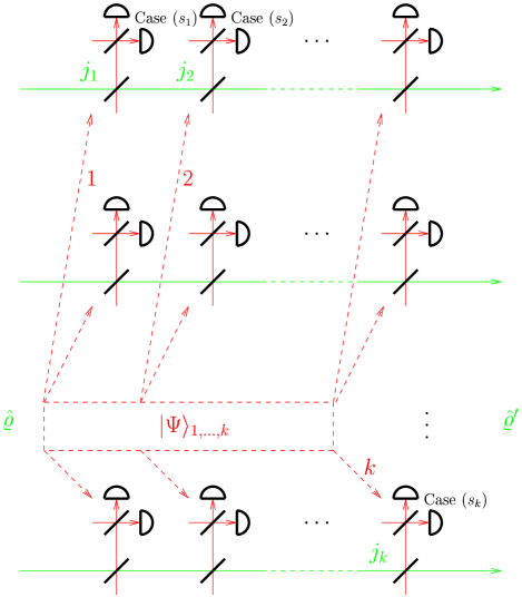
Figure 2: Example of the overall setup consisting of $k$ devices Fig. 1 applied in the signal modes $j_{1},\ldots,j_{k}$ in cases $(s_{1}),\ldots,(s_{k})$, respectively. These modes do not have to be distinct from another. The respective control input ports of the devices which are fed with states $|s\rangle$ in Fig. 1, here share an entangled state $|\Psi\rangle_{1,\ldots,k}$ given by Eq. (6).

Denoting the respective signal mode (mode 0 in Fig. 1) by $j_{l}$, we obtain a transformation in modes $j_{1},$ $\!\ldots,$ $\!j_{k}$ of the signal state $\hat{\varrho}$ according to Eq. (1), where

$$\hat{Y}(\hat{A},\alpha,\beta) = \frac{1}{\sqrt{1+|z|^{2}}}\Bigl{[}\hat{Y}_{j_{k}}^{(s_{k})}(s_{k})\cdots\hat{Y}_{j_{1}}^{(s_{1})}(s_{1})$$ (14)

$$+z\hat{Y}_{j_{k}}^{(s_{k})}(1-s_{k})\cdots\hat{Y}_{j_{1}}^{(s_{1})}(1-s_{1})\Bigr{]}$$

$$= \alpha\hat{T}(\hat{A}+\beta),$$

with

$$\hat{T} = T_{1}^{\sum_{l=1}^{k}\hat{n}_{j_{l}}},$$ (15a)

$$\hat{A} = \hat{a}_{j_{k}}^{(s_{k})}\cdots\hat{a}_{j_{1}}^{(s_{1})},$$ (15b)

$$\alpha = \frac{z}{\beta\sqrt{1+|z|^{2}}}T_{2}^{k-\sum_{l=1}^{k}s_{l}},$$ (15c)

$$\beta = zR_{1}^{-\sum_{l=1}^{k}s_{l}}\left(-\frac{T_{1}}{R_{1}^{*}}\frac{T_{2}}{R_{2}}\right)^{k-\sum_{l=1}^{k}s_{l}}$$ (15d)

$$\times T_{1}^{\sum_{r=1}^{k}\sum_{l=r}^{k}(2s_{l}-1)\delta_{j_{r},j_{l}}},$$

and $\hat{a}^{(s)}$ stands for $\hat{a}$ if $s$ $\!=$ $\!0$ and for $\hat{a}^{\dagger}$ if $s$ $\!=$ $\!1$. We see that for given beam splitter parameters $T_{k}$ and $R_{k}$, $\beta$ can be chosen as desired by varying $z$. Note that the signal modes $j_{1},$ $\!\ldots,$ $\!j_{k}$ don’t have to be distinct, cf. the examples in section VI.1 and section VI.2. Note also that those modes which are distinct may be spatially separated from each other. The signal flow of the scheme Fig. 2 then resembles that of a multi-mode quantum teleportation setup.

We now consider $N$ successive applications of Eq. (14). If $z$ is varied from step to step, the resulting overall operator becomes the product of the individual operators Eq. (14) according to

$$\hat{Y}_{\mathrm{tot}} = \hat{Y}(\hat{A},\alpha_{N},\beta_{N})\cdots\hat{Y}(\hat{A},\alpha_{1},\beta_{1})$$ (16)

$$= \hat{\prod}_{n=1}^{N}\left[\alpha_{n}\hat{T}(\hat{A}+\beta_{n})\right]$$

$$= \gamma^{\frac{N(N-1)}{2}}\hat{T}^{N}\prod_{n=1}^{N}\left[\alpha_{n}(\hat{A}+\beta_{n}\gamma^{1-n})\right]$$

$$= \gamma^{\frac{N(N-1)}{2}}\left(\prod_{n=1}^{N}\alpha_{n}\right)f_{N}^{-1}\hat{T}^{N}F_{N}(\hat{A}),$$

where $\alpha_{n}$ and $\beta_{n}$ follow according to Eqs. (15) from the parameters of $\hat{U}_{01}$ and $\hat{U}_{21}$ during the $n$’th passage and $\gamma$ is given by $\hat{A}\hat{T}$ $\!=$ $\!\gamma\hat{T}\hat{A}$, so that

$$\gamma=T_{1}^{\sum_{r=1}^{k}\sum_{l=1}^{k}(1-2s_{l})\delta_{j_{r},j_{l}}},$$ (17)

and

$$F_{N}(\hat{A})=\sum_{n=0}^{N}f_{n}\hat{A}^{n}=f_{N}\prod_{n=1}^{N}(\hat{A}+\beta_{n}\gamma^{1-n})$$ (18)

is an arbitrary polynomial of order $N$ in $\hat{A}$ determined by its roots $-\beta_{n}\gamma^{1-n}$. The product symbol $\hat{\prod}$ has been used to indicate that the index of the factors increases from right to left.

Assume now that we want to implement an arbitrary expandable function $F(\hat{A})$. In general, $\hat{A}$ can only be approximated by a polynomial $F_{N}(\hat{A})$ of order $N$ in $\hat{A}$ with sufficiently large $N$. There are however two cases in which $F(\hat{A})$ can be replaced exactly with some polynomial.

IV.1 Existence of an eigenspace of $\hat{A}$

In the first case, a set of $N^{\prime}$ $\!+$ $\!1$ eigenstates $|\varphi_{l^{\prime}}\rangle$ of $\hat{A}$ can be found,

$$\hat{A}|\varphi_{l^{\prime}}\rangle=A^{\prime}_{l^{\prime}}|\varphi_{l^{\prime}}\rangle=A_{l}|\varphi_{l^{\prime}}\rangle,\quad\begin{subarray}{c}l=0,\ldots,N\;\;,\\ l^{\prime}=0,\ldots,N^{\prime},\end{subarray}$$ (19)

where $N^{\prime}$ ($\!\geq$ $\!N$) is chosen such that a renumbering of the eigenvalues $A_{l^{\prime}}^{\prime}$ gives a set $\{A_{0},\ldots,A_{N}\}$ of exactly $N$ $\!+$ $\!1$ distinct $A_{l}$. We now choose Eq. (18) to be the polynomial

$$F_{N}(\hat{A})=\sum_{l=0}^{N}F(A_{l})\prod_{\begin{subarray}{c}k=0\\ (k\neq l)\end{subarray}}^{N}\frac{\hat{A}-A_{k}}{A_{l}-A_{k}}$$ (20)

of order $N$ in $\hat{A}$, so that we obtain $F_{N}(\hat{A})|\varphi_{l^{\prime}}\rangle$ $\!=$ $\!F(\hat{A})|\varphi_{l^{\prime}}\rangle$. In Eq. (16) we then have

$$\hat{Y}_{\mathrm{tot}}\hat{P}_{N^{\prime}}^{(j_{1},\ldots,j_{k})}=\frac{\prod_{n=1}^{N}\alpha_{n}}{f_{N}}\gamma^{\frac{N(N-1)}{2}}\hat{T}^{N}F(\hat{A})\hat{P}_{N^{\prime}}^{(j_{1},\ldots,j_{k})},$$ (21)

where

$$\hat{P}_{N^{\prime}}^{(j_{1},\ldots,j_{k})}=\sum_{l^{\prime}=0}^{N^{\prime}}|\varphi_{l^{\prime}}\rangle\langle\varphi_{l^{\prime}}|.$$ (22)

We see that a signal state $\hat{\varrho}$ satisfying the condition

$$\hat{\varrho}\hat{P}_{N^{\prime}}^{(j_{1},\ldots,j_{k})}=\hat{P}_{N^{\prime}}^{(j_{1},\ldots,j_{k})}\hat{\varrho}=\hat{\varrho}$$ (23)

is transformed according to Eq. (1), where $\hat{Y}$ $\!\sim$ $\!\hat{T}^{N}F(\hat{A})$, cf. Eq. (21). In this sense, a desired function $F(\hat{A})$ can be implemented. In order to compensate the operator $\hat{T}$, the transmittance $T_{1}$ may be chosen sufficiently close to unity, i.e., $|R_{1}|$ $\!\ll$ $\!1$. A precise compensation is possible by an additional implementation of the operator $\hat{T}^{-N}$ allowed in the photon-number truncated case as discussed below, in section VI.1. We then have $\hat{Y}$ $\!\sim$ $\!F(\hat{A})$. Note that the replacement of the function $F(\hat{A})$ by a polynomial $F_{N}(\hat{A})$ of order $N$ in $\hat{A}$ is unique. If there was another polynomial $G_{N}(\hat{A})$ of order $N$ in $\hat{A}$ for which also $G_{N}(\hat{A})|\varphi_{l^{\prime}}\rangle$ $\!=$ $\!F(\hat{A})|\varphi_{l^{\prime}}\rangle$ with $l^{\prime}$ $\!=$ $\!0,$ $\!\ldots,$ $\!N^{\prime}$, we could consider the polynomial $F_{N}(x)$ $\!-$ $\!G_{N}(x)$ of order $N$ in $x$. It has however the ($N$ $\!+$ $\!1$) distinct roots $x_{l}$ $\!=$ $\!A_{l}$, so that $F_{N}(x)$ $\!-$ $\!G_{N}(x)$ $\!\equiv$ $\!0$. Of particular interest is the case in which in each of the modes $j_{1},$ $\!\ldots,$ $\!j_{k}$, the number of annihilation operators occuring in $\hat{A}$ equals the number of creation operators, so that the eigenstates $|\varphi_{l^{\prime}}\rangle$ $\!=$ $\!|n_{j_{1}}^{(l^{\prime})},\ldots,n_{j_{k}}^{(l^{\prime})}\rangle$ are $N^{\prime}$ $\!+$ $\!1$ photon number states (they may be, e.g., the lowest states occuring in a Fock space expansion).

IV.2 Photon-number truncated signal states

In the other case, there exists a mode $j_{l}$ in which the number of annihilation operators occuring in $\hat{A}$ exceeds the number of creation operators and the signal state $\hat{\varrho}$ is photon-number truncated in this mode,

$$\hat{\varrho}\hat{P}_{N}^{(j_{l})}=\hat{P}_{N}^{(j_{l})}\hat{\varrho}=\hat{\varrho},\quad\quad\hat{P}_{N}^{(j_{l})}=\sum_{n=0}^{N}|n\rangle_{j_{l}}\,{}_{j_{l}}\langle n|.$$ (24)

We choose Eq. (18) to be the sum of the first $N$ $\!+$ $\!1$ elements of the power series expansion of $F(\hat{A})$, so that the signal state $\hat{\varrho}$ is again transformed according to Eq. (1), where $\hat{Y}$ $\!\sim$ $\!\hat{T}^{N}F(\hat{A})$, cf. Eq. (21).

V Approaching general operator functions

Assume that we want to implement an arbitrary function $\hat{F}$ of the creation and annihilation operators of a number of signal modes, $\hat{Y}$ $\!\sim$ $\!\hat{F}$ in Eq. (1). We further assume that the expansion of $\ln\hat{F}$ can according to

$$\hat{F}=\mathrm{e}^{\ln\hat{F}}=\mathrm{e}^{\sum_{n=1}^{\infty}c_{n}\hat{\mathcal{A}}_{n}}\approx\mathrm{e}^{\sum_{n=1}^{N}c_{n}\hat{\mathcal{A}}_{n}}$$ (25)

be truncated after a (sufficiently large) number $N$ of elements. Here, the $\hat{\mathcal{A}}_{n}$ are products of the respective creation and annihilation operators that can be written in the form of Eq. (15b). Consider now $N^{2}$ successive applications of Eq. (14) according to

$$\hat{Y}_{\mathrm{tot}} = \hat{Y}(\hat{A}_{N^{2}},\alpha_{N^{2}},\beta_{N^{2}})\cdots\hat{Y}(\hat{A}_{1},\alpha_{1},\beta_{1})$$ (26)

$$= \hat{\prod}_{n=1}^{N^{2}}\left[\alpha_{n}\hat{T}(\hat{A}_{n}+\beta_{n})\right]$$

$$= \hat{T}^{N^{2}}\hat{\prod}_{n=1}^{N^{2}}\left[\alpha_{n}\beta_{n}(1+\beta_{n}^{-1}\gamma_{n}^{n-1}\hat{A}_{n})\right],$$

where $\gamma_{n}$ is given by $\hat{A}_{n}\hat{T}$ $\!=$ $\!\gamma_{n}\hat{T}\hat{A}_{n}$, cf. Eq. (17). Choosing $\hat{A}_{n}$ as well as $\beta_{n}$ according to

$$\hat{A}_{n} = \hat{\mathcal{A}}_{\lceil{n}\rceil},$$ (27a)

$$\beta_{n} = Nc_{\lceil{n}\rceil}^{-1}\gamma_{n}^{n-1},$$ (27b)

where $\lceil{n}\rceil$ $\!\equiv$ $\!1$ $\!+$ $\![(n$ $\!-$ $\!1)$ $\!\mathrm{mod}$ $\!N]$, we see that

$$\hat{Y}_{\mathrm{tot}}=\biggl{(}\prod_{n=1}^{N^{2}}\alpha_{n}\beta_{n}\biggr{)}\hat{T}^{N^{2}}\hat{X},$$ (28)

where

$$\hat{X}=\left[\hat{\prod}_{n=1}^{N}\left(1+N^{-1}c_{n}\hat{\mathcal{A}}_{n}\right)\right]^{N}\stackrel{{\scriptstyle(N\gg 1)}}{{\approx}}\mathrm{e}^{\sum_{n=1}^{N}c_{n}\hat{\mathcal{A}}_{n}},$$ (29)

and therefore $\hat{X}$ $\!\approx$ $\!\hat{F}$ for $N\gg 1$. Again, we may compensate the operator $\hat{T}$ by choosing $T_{1}$ sufficiently close to unity or subsequently implementing the operator $\hat{T}^{-N^{2}}$, cf. section VI.1, so that we obtain $\hat{Y}_{\mathrm{tot}}$ $\!\sim$ $\!\hat{F}$.

VI Examples of application

We have seen that we may implement a given binomial in any moment of the creation and annihilation operators of a number of traveling optical modes. A repeated application then allows - in principle - the approximation of a desired function of the respective mode operators. In a concrete example, the general scheme can be simplified considerably. Let us illustrate this in some cases of special interest such as single- and two-mode operators, since the application of single-photon cloners may be avoided in this case.

VI.1 Functions of the single-mode photon number operator

Until now we have placed emphasis on the realization of general operators. In a given case however, the respective scheme may be simplified considerably. For example, let us assume that $\hat{A}$ $\!=$ $\!\hat{n}_{0}$. This example is of particular importance since it allows the compensation of the operators $\hat{T}$ in Eq. (16) and Eq. (28) for photon-number truncated states as we will see below. In Eq. (14), we then have $k$ $\!=$ $\!2$, $j_{1}$ $\!=$ $\!j_{2}$ $\!=$ $\!0$ and $s_{1}$ $\!=$ $\!0$, $s_{2}$ $\!=$ $\!1$. Instead of applying the setup Fig. 1 in the signal mode 0 first in case (0) and then in case (1), it is sufficient to prepare its input ports 1 and 2 in a state $|\Psi\rangle_{12}$ as defined in Eq. (7). The resulting complete setup is shown in Fig. 3(a). If the photodetectors D₁ and D₂ detect 0 and 1 photons, respectively, the signal state $\hat{\varrho}$ is transformed in mode 0 according to Eq. (1), where

$$\hat{Y}(\hat{A},\alpha,\beta) = \,{}_{1}\langle 0|\,_{2}\langle 1|\hat{U}_{21}\hat{U}_{01}|\Psi\rangle_{12}$$ (30)

$$= \alpha T_{1}^{\hat{n}_{0}}(\hat{A}-\beta),$$

with

$$\hat{A} = \hat{n}_{0},$$ (31a)

$$\alpha = -\frac{R_{2}|R_{1}|^{2}}{\sqrt{2}T_{1}},$$ (31b)

$$\beta = \left|\frac{T_{1}}{R_{1}}\right|^{2}\left(1+\frac{1}{T_{1}^{*}}\frac{T_{2}}{R_{2}}\right).$$ (31c)

For fixed $\hat{U}_{01}$, $\beta$ can be arbitrarily chosen by varying the parameters of $\hat{U}_{21}$. As a consequence, there is no need for cloning devices. In order to realize a transformation of a photon-number truncated signal state [cf. Eq. (24) with $j_{l}$ $\!=$ $\!0$] according to Eq. (1) with a desired function $\hat{Y}$ $\!\sim$ $\!F(\hat{n}_{0})$, there have to be $N$ successive applications of Eq. (30) with varying $\beta_{n}$ such that the overall operator becomes

$$\hat{Y}_{\mathrm{tot}} = \hat{Y}(\hat{A},\alpha_{N},\beta_{N})\cdots\hat{Y}(\hat{A},\alpha_{1},\beta_{1})$$ (32)

$$= \prod_{n=1}^{N}\left[\alpha_{n}T_{1}^{\hat{n}_{0}}(\hat{n}_{0}-\beta_{n})\right]$$

$$= \left(\prod_{n=1}^{N}\alpha_{n}\right)f_{N}^{-1}T_{1}^{N\hat{n}_{0}}F_{N}(\hat{n}_{0}).$$

Inserting $\hat{A}$ $\!=$ $\!\hat{n}_{0}$ and with it $A_{l}$ $\!=$ $\!l$ into Eq. (20), and furthermore substituting $T_{1}^{-Nl}F(l)$ for $F(l)$, we see that the $\beta_{n}$ in Eq. (32) must be chosen such that

$$F_{N}(\hat{n}_{0})=\frac{1}{N!}\sum_{l=0}^{N}\binom{N}{l}(-T_{1}^{N})^{-l}F(l)\prod_{\begin{subarray}{c}k=0\\ (k\neq l)\end{subarray}}^{N}(k-\hat{n}_{0}).$$ (33)

Since then $T_{1}^{N\hat{n}_{0}}F_{N}(\hat{n}_{0})|n\rangle$ $\!=$ $\!F(\hat{n}_{0})|n\rangle$ holds for number states $|n\rangle$ with $n$ $\!=$ $\!0,\ldots,N$, we obtain

$$\hat{Y}_{\mathrm{tot}}\hat{P}_{N}^{(0)}=\left(\prod_{n=1}^{N}\alpha_{n}\right)f_{N}^{-1}F(\hat{n}_{0})\hat{P}_{N}^{(0)}$$ (34)

[for $\hat{P}_{N}^{(0)}$ see Eq. (24)], where

$$f_{N}=\frac{(-1)^{N}}{N!}\sum_{l=0}^{N}\binom{N}{l}(-T_{1}^{N})^{-l}F(l),$$ (35)

so that for photon-number truncated states the desired function $F(\hat{n}_{0})$ is implemented.

As an illustration, let us consider the special case of the exponential $F(\hat{n}_{0})$ $\!=$ $\!z^{\hat{n}_{0}}$, which, if applied with appropriate $z$ in modes $j_{1},$ $\!\ldots,$ $\!j_{k}$, allows the compensation of the operators $\hat{T}$ in Eq. (16) and Eq. (28). Inserting $F(l)$ $\!=$ $\!z^{l}$ into Eq. (33) and applying

$$\sum_{k=0}^{n}(-1)^{k}\binom{k}{l}\binom{x}{k}=\frac{n+1}{x-l}(-1)^{n}\binom{n}{l}\binom{x}{n+1},$$ (36)

where $x$ is a complex number, $l$ $\!=$ $\!0,$ $\!1,\ldots$, and

$$\binom{x}{k}\equiv\left\{\begin{array}[]{r@{\quad:\quad}l}1&k=0\\ \frac{1}{k!}\prod_{j=0}^{k-1}(x-j)&k=1,2,\ldots,\end{array}\right.$$ (37)

gives

$$F_{N}(\hat{n}_{0}) = \sum_{k=0}^{N}\left(T_{1}^{-N}z-1\right)^{k}\binom{\hat{n}_{0}}{k}$$ (38)

$$= \sum_{k=0}^{N}\left(T_{1}^{-N}z-1\right)^{k}\frac{\hat{a}_{0}^{\dagger\,k}\hat{a}_{0}^{k}}{k!}.$$

Here, we have applied Eq. (69) in the case of normal ordering, $s$ $\!=$ $\!1$. Making use of Eq. (71), we see that

$$F_{N}(\hat{n}_{0})\hat{P}_{N}^{(0)} = \sum_{k=0}^{\infty}\left(T_{1}^{-N}z-1\right)^{k}\frac{\hat{a}_{0}^{\dagger\,k}\hat{a}_{0}^{k}}{k!}\hat{P}_{N}^{(0)}$$ (39)

$$= \;:\mathrm{e}^{\left(T_{1}^{-N}z-1\right)\hat{n}_{0}}:\;\hat{P}_{N}^{(0)}$$

$$= \left(T_{1}^{-N}z\right)^{\hat{n}_{0}}\hat{P}_{N}^{(0)},$$

where the symbol $:\;:$ denotes normal ordering, and Eq. (34) becomes

$$\hat{Y}_{\mathrm{tot}}\hat{P}_{N}^{(0)}=\left(\prod_{n=1}^{N}\alpha_{n}\right)N!\left(T_{1}^{-N}z-1\right)^{-N}z^{\hat{n}_{0}}\hat{P}_{N}^{(0)}.$$ (40)

VI.2 Cross-Kerr nonlinearity

Another example allowing a simplification of the general configuration is the implementation of a two-mode cross-Kerr interaction, $\hat{Y}$ $\!\sim$ $\!\mathrm{e}^{\mathrm{i}\varphi\hat{n}_{1}\hat{n}_{0}}$. In Eq. (14), we then have $\hat{A}$ $\!=$ $\!\hat{n}_{1}\hat{n}_{0}$, $k$ $\!=$ $\!4$, $j_{1}$ $\!=$ $\!j_{2}$ $\!=$ $\!0$, $j_{3}$ $\!=$ $\!j_{4}$ $\!=$ $\!1$, and $s_{1}$ $\!=$ $\!s_{3}$ $\!=$ $\!0$, $s_{2}$ $\!=$ $\!s_{4}$ $\!=$ $\!1$. Instead of applying the setup Fig. 1 in the signal modes 0 and 1 first in case (0) and then in case (1), a single application in each signal mode as shown in Fig. 3(b) is sufficient. To the setup acting on mode 1 consisting of beam splitters $\hat{U}_{15}(T_{1},R_{1})$ and $\hat{U}_{35}(T_{2},R_{2})$ as well as photodetectors D₃ and D₅, a second, identical setup acting on mode 0 is added consisting of beam splitters $\hat{U}_{04}(T_{1},R_{1})$ and $\hat{U}_{24}(T_{2},R_{2})$ as well as photodetectors D₂ and D₄. The modes are labeled as shown in Fig. 3(b).

Figure 3: Setups consisting of beam splitters $\hat{U}$ and photodetectors D, conditionally implementing a desired binomial in $\hat{n}_{0}$ (a) and a desired binomial in $(\hat{n}_{1}-\gamma)(\hat{n}_{0}-\gamma)$ with some given $\gamma$ (b).

The input modes are prepared in a state $|\Psi\rangle_{2345}$ as given by Eq. (62) with modes relabeled accordingly. If the photodetectors D₂ and D₃ detect 1 whereas D₄ and D₅ detect 0 photons, respectively, the signal state $\hat{\varrho}$ is transformed in modes 0 and 1 according to Eq. (1), where

$$\hat{Y}(\hat{A},\alpha,\beta) = \,{}_{23}\langle 1|\,_{45}\langle 0|\hat{U}_{24}\hat{U}_{04}\hat{U}_{35}\hat{U}_{15}|\Psi\rangle_{2345}$$ (41)

$$= \alpha T_{1}^{\hat{n}_{1}+\hat{n}_{0}}\bigl{(}\hat{A}-\beta\bigr{)},$$

with

$$\hat{A} = (\hat{n}_{1}-\gamma)(\hat{n}_{0}-\gamma),$$ (42a)

$$\alpha = -\frac{T_{2}^{2}}{\beta\sqrt{1+|\xi|^{2}}},$$ (42b)

$$\beta = -\frac{1}{\xi}\left(\frac{T_{1}}{|R_{1}|^{2}}\right)^{2}\left(\frac{T_{2}}{R_{2}}\right)^{2},$$ (42c)

$$\gamma = \left|\frac{T_{1}}{R_{1}}\right|^{2}.$$ (42d)

For fixed $\xi$, $T_{1}$ and $R_{1}$, $\beta$ can be chosen as desired by varying $T_{2}$ and $R_{2}$. By $N$ repeated applications of Eq. (41) with varying $\beta_{n}$ we obtain

$$\hat{Y}_{\mathrm{tot}} = \hat{Y}(\hat{A},\alpha_{N},\beta_{N})\cdots\hat{Y}(\hat{A},\alpha_{1},\beta_{1})$$ (43)

$$= \left(\prod_{n=1}^{N}\alpha_{n}\right)f_{N}^{-1}T_{1}^{N(\hat{n}_{1}+\hat{n}_{0})}F_{N}.$$

We now tune $T_{1}$ and $R_{1}$ such that $\gamma$ $\!=$ $\!\varphi^{-1}2k\pi$ with some arbitrary $k$ $\!=$ $\!1,2,\cdots$. The $\beta_{n}$ are chosen such that in Eq. (43) the polynomial $F_{N}$ of order $N$ in $\hat{A}$ becomes

$$F_{N}=\sum_{l=0}^{N}\mathrm{e}^{\mathrm{i}\varphi A_{l}}\prod_{\begin{subarray}{c}k=0\\ (k\neq l)\end{subarray}}^{N}\frac{\hat{A}-A_{k}}{A_{l}-A_{k}},$$ (44)

where $A_{0},\ldots,A_{N}$ are the ($N$ $\!+$ $\!1$) distinct values of the expression $(n_{1}-\gamma)(n_{0}-\gamma)$ with $n_{0,1}$ $\!=$ $\!0,\ldots,M$ [cf. the remarks following Eq. (19)]. On signal states $\hat{\varrho}$ whose photon number is limited to some given value $M$ in mode 0 and 1, i.e., $\hat{\varrho}$ satisfies Eq. (24), where $\hat{P}_{N}^{(j_{l})}$ is replaced with $\hat{P}_{M}^{(0)}\otimes\hat{P}_{M}^{(1)}$, Eq. (43) then acts like an operator

$$\hat{Y}_{\mathrm{tot}}=\left(\prod_{n=1}^{N}\alpha_{n}\right)f_{N}^{-1}T_{1}^{N(\hat{n}_{1}+\hat{n}_{0})}\mathrm{e}^{\mathrm{i}\varphi\hat{n}_{1}\hat{n}_{0}}.$$ (45)

In order to implement the unitary operator $\mathrm{e}^{\mathrm{i}\varphi\hat{n}_{1}\hat{n}_{0}}$, $T_{1}$ may be chosen sufficiently close to unity. Again, there is the alternative of a precise compensation of the extra exponential in Eq. (45) by an additional implementation of the operator $T_{1}^{-N(\hat{n}_{1}+\hat{n}_{0})}$ as discussed in the previous section VI.1. In this way, we have proposed a beam splitter arrangement relying on zero- and single-photon preparations and detections that acts on photon-number truncated states like a two-mode Kerr nonlinearity.

VI.3 U($N$)

Other operators whose action on photon-number truncated signal states can be realized exactly by a polynomial are those performing a U($N$) transformation. Since they can be factorized into U(2) couplers $\hat{U}_{jk}$ of the respective modes, let us limit attention to the U(2) beam splitter operator $\hat{U}_{jk}$ defined in the beginning by Eq. (3), which can equivalently be written in the form of Clausen et al. (2001),

$$\hat{U}_{jk}=(\mathcal{P}\mathcal{T})^{\hat{n}_{j}}\mathrm{e}^{-\mathcal{P}\mathcal{R}^{*}\hat{a}_{k}^{\dagger}\hat{a}_{j}}\mathrm{e}^{\mathcal{P}^{*}\mathcal{R}\hat{a}_{j}^{\dagger}\hat{a}_{k}}(\mathcal{P}^{*}\mathcal{T})^{-\hat{n}_{k}}.$$ (46)

Its parameters are here written in calligraphic style to distinguish from those of the beam splitters in the device. The implementation of exponentials of $\hat{a}_{k}^{\dagger}\hat{a}_{j}$ with $k$ $\!=$ $\!j$ explained in section VI.1 represents the case of section IV.1 and those with $k$ $\!\neq$ $\!j$ represents the case of section IV.2. Together with a detection of the vacuum state, the latter can be used to achieve a teleportation of a state $\hat{\varrho}$ from mode $j$ to mode $k$,

$$\hat{\varrho}_{k}=\hat{I}_{kj}\hat{\varrho}_{j}\hat{I}_{jk},$$ (47)

where

$$\hat{I}_{kj}=\sum_{n=0}^{\infty}|n\rangle_{k}\,{}_{j}\langle n|=\,_{j}\langle 0|\mathrm{e}^{\hat{a}_{k}^{\dagger}\hat{a}_{j}}|0\rangle_{k}=\hat{I}_{jk}^{\dagger}.$$ (48)

A comparison with Eq. (46) shows that $\exp(\hat{a}_{k}^{\dagger}\hat{a}_{j})$ [or $\exp(\hat{a}_{j}^{\dagger}\hat{a}_{k})$] is realized for $\mathcal{T}$ $\!=$ $\!0$. Physically, the beam splitter then describes a mirror. Since Eq. (46) becomes singular in this case, we have to construct it by a successive implementation of two operators Eq. (46) whose combined action results according to

$$\hat{U}_{jk}(\mathcal{T}_{2},\mathcal{R}_{2},\mathcal{P}_{2})\hat{U}_{jk}(\mathcal{T}_{1},\mathcal{R}_{1},\mathcal{P}_{1})$$ (49)

$$= \hat{U}_{jk}(\mathcal{T}_{2}\mathcal{T}_{1}-\mathcal{R}_{2}\mathcal{R}_{1}^{*},\mathcal{T}_{2}\mathcal{R}_{1}+\mathcal{R}_{2}\mathcal{T}_{1}^{*},\mathcal{P}_{2}\mathcal{P}_{1})$$

again in a U(2) beam splitter operator. Choosing $\mathcal{T}_{j}$ $\!=$ $\!\mathcal{R}_{j}$ $\!=$ $\!1/\sqrt{2}$ and $\mathcal{P}_{j}$ $\!=$ $\!1$, we get an operator $\hat{U}_{jk}(0,1,1)$. If implemented by our scheme with separated modes $j$ and $k$, such a ‘quantum mirror’  realizes a bidirectional teleportation between these modes.

More generally, we may consider a transformation in $N$ modes $j$ $\!=$ $\!1,\ldots,N$ of a signal according to (1) by an operator $\hat{Y}$ $\!\sim$ $\!\hat{U}$ whose action is defined by

$$\hat{U}^{\dagger}\hat{a}_{j}\hat{U}=\hat{a}_{p(j)},$$ (50)

where $p(1),\ldots,p(N)$ is a permutation of $1,\ldots,N$. The set of such permutations of $N$ mode indices forms the discrete symmetric subgroup S($N$) of U($N$) physically representing $N$-mode mirrors (with the identical operation included). Note that in general we may add additional phase shifts according to $\hat{U}^{\prime}$ $\!=$ $\!\mathrm{e}^{\mathrm{i}\sum_{j=1}^{N}\varphi_{j}\hat{n}_{j}}\hat{U}$, so that S($N$) is replaced with U(1)${}^{N}\,\otimes\,$S($N$). If $\hat{U}$ is implemented by the setup Fig. 2 with spatially separated signal modes, then we again have the situation of a teleportation. One possibility to construct $\hat{U}$ is to introduce auxiliary modes $-1,\ldots,-N$, and to apply (48) repeatedly according to

$$\hat{U}=\hat{I}_{p(N),-N}\cdots\hat{I}_{p(1),-1}\hat{I}_{-N,N}\cdots\hat{I}_{-1,1}.$$ (51)

VI.4 Preparation of multi-photon entangled states

We conclude with an example of state preparation which may be understood as a state transformation with a given input state. Consider the following situation. By feeding the overall setup with vacuum, $\hat{\varrho}$ $\!=$ $\!|0\rangle\langle 0|$, the scheme may be used to generate a state difficult to prepare by other means. An example are $k$-mode states

$$|z\rangle_{1,\ldots,k} = \sqrt{\frac{1-|z|^{2}}{1-|z|^{2(N+1)}}}\sum_{n=0}^{N}z^{n}|n\rangle_{1,\ldots,k}$$

$$= \frac{1}{\sqrt{p}}\hat{Y}|0\rangle_{1,\ldots,k},$$

which can be generated by applying a polynomial

$$\hat{Y}\sim\sum_{n=0}^{N}n!^{-\frac{k}{2}}(z\hat{A})^{n}$$ (53)

in $\hat{A}$ $\!=$ $\!\hat{a}_{k}^{\dagger}\cdots\hat{a}_{1}^{\dagger}$ to the vacuum. The states Eq. (VI.4) are of interest from the theoretical point of view. Consider the case $|z|$ $\!\leq$ $\!1$ and $N$ $\!\to$ $\!\infty$. We see that for $k$ $\!=$ $\!1$ we obtain a coherent phase state (in particular, for $|z|$ $\!=$ $\!1$ a London phase state). For $k$ $\!=$ $\!2$ we obtain a two-mode squeezed state (in particular, for $|z|$ $\!=$ $\!1$ an EPR-like state). In the limit $k$ $\!\to$ $\!\infty$, the states Eq. (VI.4) may be used as a representation of an EPR-like state between a number $n$ of quantum fields (instead of two modes of a field). To see this, the fields are indexed according to $\lceil{j}\rceil$ $\!\equiv$ $\!1$ $\!+$ $\![(j$ $\!-$ $\!1)$ $\!\mathrm{mod}$ $\!n]$, i.e., mode $j$ is ascribed to field $\lceil{j}\rceil$.

VII Conclusion

In summary it can be said that, starting from a single photon, cf. Eq. (7), we can with a given probability approach arbitrary operators of spatially separated traveling optical modes. The problem is that the success probability, which depends on the desired transformation and the signal state in general, is expected to decline exponentially with an increasing number of steps $N$, so that the practical applicability of the scheme is limited to small $N$, sufficient to engineer, e.g., states in the vicinity of the vacuum. On the other hand, the application of giant nonlinearities to fields containing only few photons represents just the case discussed in potential quantum information processing devices. To give an estimation, consider a passively mode-locked laser whose resonator has an optical round trip length of $l$ = 3 cm, so that the repetition frequency of the emitted pulse train is $\nu$ = $l^{-1}c$ = 10 GHz. If this pulse train is used to prepare the entangled state needed to run the scheme, then its repetition frequency determines that of the overall device. An assumed total success probability of $p$ $\!=$ $\!10^{-10}$ would then reduce the mean repetition frequency of the properly transformed output pulses to $\nu^{\prime}$ = 1 Hz, which may still be useful for basic research experiments but unacceptable for technical applications. Apart from this, there may be the situation where only a single unknown signal pulse is available that must not be spoiled by a wrong detection since no copies can be produced of it. This constitutes the main drawback of all conditional measurement schemes.

It may be worth mentioning that the whole scheme may also run ‘time-reversed’ , i.e., all pulses are sent in opposite directions through the device, while the locations of state preparations and (assumed) detections are interchanged, so that the resulting ‘adjoint’  scheme implements the adjoint operator $\hat{Y}^{\dagger}$.

Appendix A Single-photon cloning

In what follows, we give a number of possibilities to implement a single-photon cloner Eq. (8).

A.1 Cross-Kerr nonlinearity

To implement single-photon cloning, we may apply a Mach-Zehnder-interferometer equipped with a cross-Kerr nonlinearity as can be seen as follows. We prepare input mode 2 of a balanced beam splitter $\hat{U}_{21}(T$ $\!=$ $\!-R$ $\!=$ $\!1/\sqrt{2})$ in a single-photon state $|1\rangle$ and the other input mode in the vacuum state $|0\rangle$. After output mode 2 has passed a cross-Kerr coupler

$$\hat{U}_{02}=\mathrm{e}^{\mathrm{i}\pi\hat{n}_{2}\hat{n}_{0}},$$ (54)

it is remixed with output mode 1 at a second beam splitter $\hat{U}_{21}^{\dagger}$. The output mode 2 of this second beam splitter is then again mixed with an auxiliary mode 3 prepared in a coherent state $|\xi\rangle$ with $\xi$ $\!=$ $\!T^{-1}R$ using a beam splitter $\hat{U}_{32}(T,R)$. If eventually 0 and 1 photons are detected in modes 2 and 3, respectively, the action of the complete setup on the state of the input mode 0 can be described by an operator

$$\hat{Y} = \,{}_{2}\langle 0|\,_{3}\langle 1|\hat{U}_{32}\hat{U}_{21}^{\dagger}\hat{U}_{02}\hat{U}_{21}|0\rangle_{1}|1\rangle_{2}|\xi\rangle_{3}$$ (55)

$$= \mathrm{e}^{\mathrm{i}\arg{R}}\sqrt{p}\,\sum_{s=0}^{1}\frac{1+(-1)^{\hat{n}_{0}+s}}{2}|s\rangle_{1},$$

so that

$$\hat{Y}\hat{P}_{1}^{(0)}=\mathrm{e}^{\mathrm{i}\arg{R}}\sqrt{p}\;\hat{Q}_{10}$$ (56)

[for $\hat{P}_{1}^{(0)}$ see Eq. (24)]. The success probability

$$p=\left[(1+|\xi|^{-2})\mathrm{e}^{|\xi|^{2}}\right]^{-1}$$ (57)

attains for $|\xi|^{2}$ $\!=$ $\!(\sqrt{5}-1)/2$ $\!\approx$ $\!0.62$ its maximum value of $p_{\mathrm{max}}$ $\!\approx$ $\!0.21$.

A.2 Three-wave-mixer

A disadvantage of the above proposal is its dependency on a given measurement result. Unitary photon cloning can be achieved using a three-wave-mixer

$$\hat{U}_{012}(\varphi)=\mathrm{e}^{\mathrm{i}\varphi(\hat{a}_{0}\hat{a}_{1}^{\dagger}\hat{a}_{2}^{\dagger}+\hat{a}_{0}^{\dagger}\hat{a}_{1}\hat{a}_{2})}.$$ (58)

Preparing its input mode 0 in a photon number state $|s\rangle$ with $s$ $\!=$ $\!0,1$ and its input modes 1 and 2 in the vacuum state $|0\rangle$, the output state becomes

$$\hat{U}_{012}(\varphi)|s\rangle_{0}|0\rangle_{12}=\cos(s\varphi)|s\rangle_{0}|0\rangle_{12}+\mathrm{i}\sin(s\varphi)|0\rangle_{0}|s\rangle_{12},$$ (59)

so that for a phase of $\varphi$ $\!=$ $\!\pi/2$ and an additional application of a preceding phase shifter $\mathrm{e}^{-\mathrm{i}\frac{\pi}{2}\hat{n}_{0}}$ we obtain an output state $\hat{Y}|s\rangle_{0}$ $\!=$ $\!|s\rangle_{12}$, where

$$\hat{Y}=\,_{0}\langle 0|\hat{U}_{012}(\pi/2)\mathrm{e}^{-\mathrm{i}\frac{\pi}{2}\hat{n}_{0}}|0\rangle_{12}.$$ (60)

After relabeling output mode 2 as 0 we get

$$\hat{Y}\hat{P}_{1}^{(0)}=\hat{Q}_{10},$$ (61)

cf. Eq. (8) and Eq. (24). Formally, we could consider a success probability for which $p$ $\!=$ $\!\,{}_{0}\langle s|\hat{Y}^{\dagger}\hat{Y}|s\rangle_{0}$ $\!=$ $\!1$ holds as expected for an unconditional unitary operation.

A.3 Linear optics

A disadvantage of the previous two proposals is their dependency on large nonlinear coefficients which are hardly achievable in practice. Therefore, we now give a possibility of implementing Eq. (8) solely based on beam splitters and zero- and single-photon detections. Assume that a state

$$|\Psi\rangle_{1234}=\frac{|1\rangle_{12}|0\rangle_{34}+\xi\,|0\rangle_{12}|1\rangle_{34}}{\sqrt{1+|\xi|^{2}}}$$ (62)

with some arbitrary $\xi$ $\!\neq$ $\!0$ is prepared. Mode 3 is mixed with an auxiliary mode 5 prepared in a coherent state $|\xi\rangle$ using a beam splitter $\hat{U}_{53}(T$ $\!=$ $\!R$ $\!=$ $\!1/\sqrt{2})$ and mode 4 passes a beam splitter $\hat{U}_{04}(T$ $\!=$ $\!R$ $\!=$ $\!1/\sqrt{2})$. If eventually 0 photons are detected in modes 3 and 4 but 1 photon in each of the modes 0 and 5, respectively, the device realizes an operator

$$\hat{Y} = \,{}_{34}\langle 0|\,_{05}\langle 1|\hat{U}_{04}\hat{U}_{53}|\Psi\rangle_{1234}|\xi\rangle_{5}$$ (63)

$$= \mathrm{e}^{\mathrm{i}\arg{\xi}}\sqrt{p}\,\hat{Q}_{10}$$

that acts on states $|s\rangle$ in which input port 0 of the beam splitter $\hat{U}_{04}$ is prepared. Note that in the second line of Eq. (63) we have relabeled output mode 2 as mode 0. The success probability

$$p=\left[4(1+|\xi|^{-2})\mathrm{e}^{|\xi|^{2}}\right]^{-1}$$ (64)

becomes maximum for $|\xi|^{2}$ $\!=$ $\!(\sqrt{5}-1)/2$ $\!\approx$ $\!0.62$ for which $p$ $\!\approx$ $\!0.05$.

One way to prepare the state Eq. (62) from single-photon states is shown in Fig. 4. If transmittance and reflectance of the beam splitter $\hat{U}_{04}$ are denoted by $T$ and $R$, respectively, then those of beam splitter $\hat{U}_{35}$ are given by $T^{*}$ and $R^{*}$. The parameters of all other beam splitters are given by $T$ $\!=$ $\!R$ $\!=$ $\!1/\sqrt{2}$.

Figure 4: Setup consisting of beam splitters $\hat{U}$ and photodetectors D, conditionally preparing a state given by Eq. (62).

The setup represents an array of these beam splitters which is fed with a number of single-photon states $|1\rangle$ and vacuum states $|0\rangle$ as shown in the figure. If each of the two photodetectors detects 1 photon, the output state becomes

$$\frac{\mathrm{e}^{\mathrm{i}\varphi}}{\sqrt{p}}\,_{05}\langle 1|\hat{U}_{50}\hat{U}_{34}\hat{U}_{04}\hat{U}_{35}\hat{U}_{12}\hat{U}_{02}\hat{U}_{15}|1\rangle_{0125}|0\rangle_{34}=|\Psi\rangle_{1234},$$ (65)

where $\varphi$ $\!=$ $\!\pi$ $\!-$ $\!2\arg{T}$ is an unrelevant phase and

$$\xi=-R^{*2}.$$ (66)

The success probability reads

$$p=\left(\frac{1-|\xi|}{2}\right)^{2}(1+|\xi|^{2}).$$ (67)

We see that $p$ drops from its maximum value of 0.25 as attained for $\xi$ $\!=$ $\!0$ to 0 if $|\xi|$ $\!\to$ $\!1$. For the above value of $|\xi|^{2}$ $\!=$ $\!0.62$ we obtain $p$ $\!\approx$ $\!0.02$.

Appendix B $s$-ordering relations for the photon number operator

In what follows, we compile some relations regarding the $s$-ordering of the photon number operator $\hat{n}$ $\!=$ $\!\hat{a}^{\dagger}\hat{a}$ as used in section VI.1. We start with its $k$th power. Introducing $s$-ordering according to Cahill and Glauber (1969),

$$\{\hat{a}^{\dagger\,m}\hat{a}^{n}\}_{s}=\!\!\!\sum_{k=0}^{\min[m,n]}k!\binom{m}{k}\!\binom{n}{k}\!\left(\frac{t\!-\!s}{2}\right)^{k}\{\hat{a}^{\dagger\,m-k}\hat{a}^{n-k}\}_{t},$$ (68)

and applying Prudnikov et al. (1986), p. 626, no. 30, we get

$$\left\{\hat{n}^{k}\right\}_{s} = k!\sum_{l=0}^{k}\left(\frac{1\!-\!s}{2}\right)^{k-l}\binom{k}{l}\binom{\hat{n}}{l}$$ (69)

$$= k!\left(-\frac{s\!+\!1}{2}\right)^{k}\mathrm{P}_{k}^{(0,\hat{n}-k)}\!\left(\frac{s\!-\!3}{s\!+\!1}\right).$$

The inverse relation is obtained from Eq. (68) with $s$ $\!=$ $\!1$ and $t$ renamed as $s$, inserting Eq. (69) with $s$ $\!=$ $\!1$, and applying Prudnikov et al. (1986), p. 624, no. 25, as well as p. 614, no. 31, which yields

$$\hat{n}^{k}\! = \!\left\{\sum_{m,j,l=0}^{k}\binom{j}{m}\!\binom{j}{l}\!(-1)^{m+j}m^{k}\!\left(\frac{s\!-\!1}{2}\right)^{j-l}\frac{\hat{n}^{l}}{l!}\right\}_{s}\;\;\;\;$$ (70)

$$= \!\left\{\sum_{m,j=0}^{k}\binom{j}{m}(-1)^{m}m^{k}\left(\frac{1\!-\!s}{2}\right)^{j}\mathrm{L}_{j}\!\left(\frac{2\hat{n}}{1\!-\!s}\right)\right\}_{s}\!\!\!\!.$$

To consider the case where $\hat{n}$ is the exponent, we apply Prudnikov et al. (1986), p. 709, no. 3, as well as p. 612, no. 1, to Eq. (69), which gives

$$\left\{\mathrm{e}^{\alpha\hat{n}}\right\}_{s}=\frac{\left(1+\frac{s+1}{2}\alpha\right)^{\hat{n}}}{\left(1+\frac{s-1}{2}\alpha\right)^{\hat{n}+1}}.$$ (71)

The inverse relation

$$\alpha^{\hat{n}}=\left\{\frac{\mathrm{e}^{\left(\frac{1}{\alpha-1}+\frac{1-s}{2}\right)^{-1}\hat{n}}}{1+\frac{(1-s)(\alpha-1)}{2}}\right\}_{s}$$ (72)

then follows directly from Eq. (71) in accordance with Cahill and Glauber (1969).

References

- Lloyd (1994) S. Lloyd, J. Mod. Opt. 41, 2503 (1994).
- Lloyd (1995) S. Lloyd, Phys. Rev. Lett. 75, 346 (1995).
- Lloyd and Braunstein (1999) S. Lloyd and S. L. Braunstein, Phys. Rev. Lett. 82, 1784 (1999).
- Lloyd and Slotine (2000) S. Lloyd and J.-J. E. Slotine, Phys. Rev. A 62, 012307 (2000).
- Lloyd (2000) S. Lloyd, Phys. Rev. A 62, 022108 (2000).
- Lloyd and Viola (2001) S. Lloyd and L. Viola, Phys. Rev. A 65, 010101(R) (2001).
- Vogel et al. (1993) K. Vogel, V. M. Akulin, and W. P. Schleich, Phys. Rev. Lett. 71, 1816 (1993).
- Harel and Akulin (1999) G. Harel and V. M. Akulin, Phys. Rev. Lett. 82, 1 (1999).
- Kurizki et al. (2000) G. Kurizki, A. Kozhekin, and G. Harel, Opt. Comm. 179, 371 (2000).
- Akulin et al. (2001) V. M. Akulin, V. Gershkovich, and G. Harel, Phys. Rev. A 64, 012308 (2001).
- Solomon and Schirmer (2002) A. I. Solomon and S. G. Schirmer, Int. J. Mod. Phys. B 16, 2107 (2002).
- Schirmer et al. (2002a) S. G. Schirmer, A. D. Greentree, V. Ramakrishna, and H. Rabitz, J. Phys. A: Math. Gen. 35, 8315 (2002a).
- Schirmer et al. (2002b) S. G. Schirmer, A. I. Solomon, and J. V. Leahy, J. Phys. A: Math. Gen. 35, 8551 (2002b).
- Drobný et al. (1998) G. Drobný, B. Hladký, and V. Bužek, Phys. Rev. A 58, 2481 (1998).
- Drobný et al. (1999) G. Drobný, B. Hladký, and V. Bužek, Acta Phys. Slov. 49, 665 (1999).
- Hladký et al. (2000) B. Hladký, G. Drobný, and V. Bužek, Phys. Rev. A 61, 022102 (2000).
- Kok and Braunstein (2001) P. Kok and S. L. Braunstein, J. Phys. A: Math. Gen. 34, 6185 (2001).
- Fiurášek and Peřina (2000) J. Fiurášek and J. Peřina, Phys. Rev. A 62, 033808 (2000).
- Wallentowitz and Vogel (1997) S. Wallentowitz and W. Vogel, Phys. Rev. A 55, 4438 (1997).
- Reck et al. (1994) M. Reck, A. Zeilinger, H. J. Bernstein, and P. Bertani, Phys. Rev. Lett. 73, 58 (1994).
- Knill et al. (2001) E. Knill, R. Laflamme, and G. J. Milburn, Nature 409, 46 (2001).
- Steuernagel (1997) O. Steuernagel, Opt. Comm. 138, 71 (1997).
- Paris (2000) M. G. A. Paris, Phys. Rev. A 62, 033813 (2000).
- Ş. K. Özdemir et al. (2001) Ş. K. Özdemir, A. Miranowicz, M. Koashi, and N. Imoto, Phys. Rev. A 64, 063818 (2001).
- Zou et al. (2002a) X. B. Zou, K. Pahlke, and W. Mathis, Phys. Rev. A 66, 014102 (2002a).
- Zou et al. (2002b) X. B. Zou, K. Pahlke, and W. Mathis, Phys. Rev. A 66, 044302 (2002b).
- Zou et al. (2002c) X. B. Zou, K. Pahlke, and W. Mathis, Phys. Lett. A 306, 10 (2002c).
- Lee et al. (2002) H. Lee, P. Kok, N. J. Cerf, and J. P. Dowling, Phys. Rev. A 65, 030101(R) (2002).
- Fiurášek (2002) J. Fiurášek, Phys. Rev. A 65, 053818 (2002).
- Koashi et al. (2001) M. Koashi, T. Yamamoto, and N. Imoto, Phys. Rev. A 63, 030301(R) (2001).
- Ralph et al. (2001) T. C. Ralph, A. G. White, W. J. Munro, and G. J. Milburn, Phys. Rev. A 65, 012314 (2001).
- Pittman et al. (2001) T. B. Pittman, B. C. Jacobs, and J. D. Franson, Phys. Rev. A 64, 062311 (2001).
- Zou et al. (2002d) X. B. Zou, K. Pahlke, and W. Mathis, Phys. Rev. A 65, 064305 (2002d).
- Ralph et al. (2002) T. C. Ralph, N. K. Langford, T. B. Bell, and A. G. White, Phys. Rev. A 65, 062324 (2002).
- Zou et al. (2002e) X. B. Zou, K. Pahlke, and W. Mathis, Phys. Rev. A 66, 064302 (2002e).
- Pan et al. (2001) J.-W. Pan, C. Simon, Č. Brukner, and A. Zeilinger, Nature 410, 1067 (2001).
- Gottesman et al. (2001) D. Gottesman, A. Kitaev, and J. Preskill, Phys. Rev. A 64, 012310 (2001).
- Dušek (2001) M. Dušek, Opt. Comm. 199, 161 (2001).
- Calsamiglia (2002) J. Calsamiglia, Phys. Rev. A 65, 030301(R) (2002).
- Dakna et al. (1998) M. Dakna, L. Knöll, and D.-G. Welsch, Europ. Phys. Journ. D 3, 295 (1998).
- Calsamiglia et al. (2001) J. Calsamiglia, S. M. Barnett, N. Lütkenhaus, and K.-A. Suominen, Phys. Rev. A 64, 043814 (2001).
- Fiurášek et al. (2002) J. Fiurášek, S. Iblisdir, S. Massar, and N. J. Cerf, Phys. Rev. A 65, 040302 (2002).
- Clausen et al. (2001) J. Clausen, H. Hansen, L. Knöll, J. Mlynek, and D.-G. Welsch, Appl. Phys. B 72, 43 (2001).
- Cahill and Glauber (1969) K. E. Cahill and R. J. Glauber, Phys. Rev. 177, 1857 (1969).
- Prudnikov et al. (1986) A. P. Prudnikov, Y. A. Brychkov, and O. I. Marichev, Integrals and Series, vol. 1: Elementary Functions (Gordon and Breach Science Publishers, Amsterdam, 1986).