Quantised Three-Pillar Problem

Abstract

This paper examines the quantum mechanical system that arises when one quantises a classical mechanical configuration described by an underdetermined system of equations. Specifically, we consider the well-known problem in classical mechanics in which a beam is supported by three identical rigid pillars. For this problem it is not possible to calculate uniquely the forces supplied by each pillar. However, if the pillars are replaced by springs, then the forces are uniquely determined. The three-pillar problem and its associated indeterminacy is recovered in the limit as the spring constant tends to infinity. In this paper the spring version of the problem is quantised as a constrained dynamical system. It is then shown that as the spring constant becomes large, the quantum analog of the ambiguity reemerges as a kind of quantum anomaly.

Consider a rigid beam of weight $W$ supported by three identical incompressible pillars (see Fig. 1). Let the upward forces provided by the pillars be $F_{1}$, $F_{2}$, and $F_{3}$, respectively. If the beam is in static equilibrium, then the sum of the upward forces must equal $W$:

$$F_{1}+F_{2}+F_{3}=W.$$ (1)

Also, the torque on the beam about any point must vanish. If we calculate the torque about the centre, we obtain the condition

$$F_{1}=F_{3}.$$ (2)

(Calculating the torque about any other point does not give additional information). The simultaneous solution to (1) and (2) is

$$F_{1} = {1\over 2}(W-f),$$

$$F_{2} = f,$$

$$F_{3} = {1\over 2}(W-f),$$ (3)

where $f$ is an arbitrary force that cannot be determined by the conditions of the problem. This is an elementary example of a classical mechanical system whose physical characteristics are underdetermined.

Figure 1: Three-pillar problem: an elementary example of a classical mechanical system characterised by an underdetermined set of equations. A beam in static equilibrium is supported by three identical incompressible pillars. The condition of static equilibrium is described by two equations, the force balance and the torque balance. However, there are three unknowns, the upward forces $F_{1}$, $F_{2}$, and $F_{3}$ provided by the three pillars. As a consequence, the forces cannot be determined by the equations of classical mechanics.

It is possible to reformulate the three-pillar problem in such a way as to remove this ambiguity. We replace the three pillars by three identical springs having spring constant $k$. Now, the rigid beam rests on these springs, and the springs are displaced from their equilibrium lengths by the amounts $x$, $y$, and $z$ (see Fig. 2). For this problem we can determine $x$, $y$, and $z$, and thus we can determine the forces uniquely. The force balance equation reads

$$kx+ky+kz=W,$$ (4)

and the torque balance condition implies that

$$x=z.$$ (5)

The condition that the beam is straight and rigid implies that

$$x+z=2y,$$ (6)

which is a new equation having no analogue in the three-pillar problem. The simultaneous solution of equations (4) – (6) gives $x=y=z={W\over 3k}$, and thus the upward forces imposed on the beam by the three springs are

$$F_{1}={1\over 3}W,\qquad F_{2}={1\over 3}W,\qquad F_{3}={1\over 3}W.$$ (7)

The ambiguity in the three-pillar problem is eliminated because the flexibility in the springs and the rigidity of the beam give rise to the additional condition (6) that allows us to solve for the forces. Thus, if the pillars are replaced by compressible objects, which need not even be identical, then the indeterminacy is lifted. However, if we take the limit $k\to\infty$ in the spring problem, then the springs become rigid objects, and we recover the three-pillar problem. To see this, we note from (4) that the limit $k\to\infty$ gives

$$x+y+z=0$$ (8)

because $W$ is a constant. The torque condition (5) is still valid, and along with (6) we find that $x=y=z=0$. We obtain this result because in this limit the springs become incompressible, and the deviation from the equilibrium length of the springs must vanish. However, the forces are no longer determined because they are expressed in the ambiguous form $F_{i}=\infty\times 0$ ($i=1,2,3$). Thus, any values for the forces are allowed subject to constraints (1) and (2).

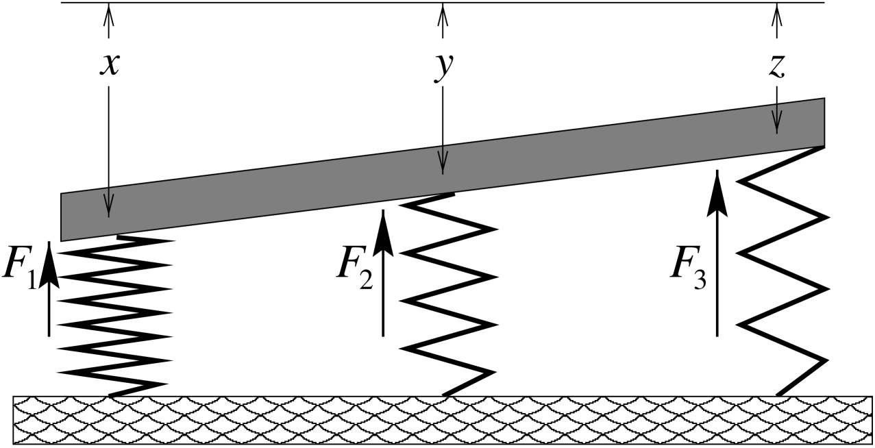
Figure 2: Three spring problem: the rigid pillars in Fig. 1 are replaced by identical springs having spring constant $k$. The classical equations describing the system in static equilibrium have a unique solution. The beam is shown resting on the springs whose displacements from equilibrium are $x$, $y$, and $z$. The displacements are determined to be $x=y=z=W/(3k)$. Thus, the forces provided by the springs are uniquely determined to be $W/3$ and the ambiguity in the three-pillar problem is removed.

Let us now consider the quantum mechanical version of the three-spring problem. To describe the quantised three-spring problem we start with the Hamiltonian

$$H={1\over 2m}\left(p_{x}^{2}+p_{y}^{2}+p_{z}^{2}\right)+{1\over 2}k\left(x^{2}+y^{2}+z^{2}\right),$$ (9)

which represents three uncoupled harmonic oscillators. Note that we have shifted the zeros of the variables $x$, $y$, and $z$ by the amount ${W\over 3k}$ so that the beam oscillates about its classical resting position. We then impose the constraint (6) to eliminate the dynamical variable $y$. The Hamiltonian thus obtained is

$$H={1\over 2m}\left[p_{x}^{2}+{1\over 2}\left(p_{x}+p_{z}\right)^{2}+p_{z}^{2}\right]+{1\over 2}k\left[x^{2}+{1\over 4}(x+z)^{2}+z^{2}\right].$$ (10)

It is convenient to make the change of variables $r=x+z$ and $s=x-z$. The variable $r$ represents vertical oscillatory motion of the centre of mass of the beam and the variable $s$ is associated with the rotational motion of the beam. In terms of these variables, the resulting Hamiltonian is diagonal and we obtain the time-independent Schrödinger equation

$$\left[-{1\over 2m}\left(3{\partial^{2}\over\partial r^{2}}+2{\partial^{2}\over\partial s^{2}}\right)+{1\over 8}k\left(3r^{2}+2s^{2}\right)\right]\psi(r,s)=E\psi(r,s).$$ (11)

Let us calculate the expectation value of the force, given by the negative derivative of the potential, applied by the central oscillator. We perform this calculation in the ground state of the quantum system. The (unnormalised) ground-state wave function is

$$\psi_{0}(r,s)=\exp\left(-{1\over 4}\sqrt{km}\,r^{2}\right)\exp\left(-{1\over 4}\sqrt{km}\,s^{2}\right).$$ (12)

The expectation value of force in the central oscillator, taking into account the shift of the zero, is given by $W/3$ plus the integral

$$\langle 0|{\rm Force}|0\rangle = -\frac{k}{2}{\int\int{\rm d}r\,r\,{\rm d}s\,\exp\left[-{1\over 2}\sqrt{mk}\left(r^{2}+s^{2}\right)\right]\over\int\int{\rm d}r\,{\rm d}s\,\exp\left[-{1\over 2}\sqrt{mk}\left(r^{2}+s^{2}\right)\right]}$$ (13)

$$= -\frac{k}{2}{\int{\rm d}r\,r\,\exp\left(-{1\over 2}\sqrt{mk}\,r^{2}\right)\over\int{\rm d}r\,\exp\left(-{1\over 2}\sqrt{mk}\,r^{2}\right)},$$

where we have divided out the integral over the variable $s$. So long as the spring constant $k$ is finite, a reflection symmetry argument implies that the integral in the numerator vanishes. Indeed, in any state, the expectation value of $r$ vanishes by reflection symmetry. However, as $k\to\infty$, the expression in (13) is the product of 0 and $\infty$, and we have obtained an ambiguous result.

This ambiguity may be regarded as a kind of quantum anomaly. Typically, in quantum field theory one encounters anomalies for which there is a divergent integral multiplying a quantity that vanishes because of a geometrical symmetry argument. For example, in the Schwinger model of two-dimensional electrodynamics the trace of the photon propagator formally vanishes by the symmetry properties of two-dimensional gamma matrices [1]. However, the photon propagator contains an integral that is logarithmically divergent. There are many tricks that can be used to regulate and then calculate such ambiguous quantities. In the case of the Schwinger model one can regulate the divergent integral by performing the calculation in $2+\epsilon$ dimensions; in $2+\epsilon$ dimensions the trace of the gamma matrices does not vanish and the integral is finite. One then takes the limit $\epsilon\to 0$ to calculate the value of the anomaly. Another example of an anomaly is the so-called trace anomaly, where the stress-energy tensor formally has a vanishing trace, but is represented by a divergent integral [2].

We view the expression in (13) as a kind of quantum anomaly because there is one quantity (here, the integral) that vanishes by a geometrical symmetry argument (reflection of $r$). This quantity is multiplied by a second factor $k$ that diverges (here, $k\to\infty$). Our objective is to demonstrate that, depending on the regularisation scheme chosen, we can get any result for the expectation value (13) of the force.

As an example, we can regulate the anomalous ambiguous product

$$A=\lim_{\Lambda\to\infty}\Lambda\int_{-\infty}^{\infty}{\rm d}r\,re^{-r^{2}}$$ (14)

as follows:

$$A\equiv\lim_{\Lambda\to\infty}\Lambda\int_{-\infty}^{\sqrt{\log[\Lambda/(2a)]}}{\rm d}r\,re^{-r^{2}},$$ (15)

where $a>0$ is arbitrary. Evaluating (15) exactly, we obtain

$$A=-a.$$ (16)

Apparently, by choosing an appropriate regulation scheme we can obtain any value $-a$ for $A$. Since the expression for the force in (13) has the form of the anomalous product in (14), we see that as the spring constant $k$ tends to infinity, the expectation value of the force is arbitrary.

We wish to express our gratitude to H. F. Jones for his stimulating suggestions. DCB gratefully acknowledges financial support from The Royal Society. This work was supported in part by the U.S. Department of Energy.

References

- [1] Schwinger, J 1962 Phys. Rev. 128 2425
- [2] Coleman, S 1972 In Developments in high-energy physics Academic Press: New York