Equivalence between the real time Feynman histories and the quantum shutter approaches for the “passage time” in tunneling

Abstract

We show the equivalence of the functions $G_{\rm p}(t)$ and $|\Psi(d,t)|^{2}$ for the “passage time” in tunneling. The former, obtained within the framework of the real time Feynman histories approach to the tunneling time problem, using the Gell-Mann and Hartle’s decoherence functional, and the latter involving an exact analytical solution to the time-dependent Schrödinger equation for cutoff initial waves.

I INTRODUCTION

The tunneling time problem has remained a controversial issue after the question of how long it takes a particle to traverse a classically forbidden region, was raised 70 years ago maccoll . There are a number of approaches to this problem review . In this paper, an unexpected close relationship is found between a real time Feynman path integral approach yamadapra ; yamada ; yamadaun and the quantum shutter approach gcr97 ; gcv01 , which are, at first sight, unlikely to be related.

If we use the real time Feynman path integrals feynman , we can define the “amplitude distribution” of tunneling time as the sum of $e^{iS/\hbar}$ ($S$ being the action) over the paths that take a specified amount of time to traverse the barrier region. With the amplitude distribution, we can deal with the interesting question whether or not a probability distribution is definable for tunneling time intrinsic . The definability of the probability distribution depends on whether or not the amplitude distribution has the property of orthogonality, i.e., whether or not the classes of Feynman paths taking time $\tau_{1}$ and $\tau_{2}$ ($\tau_{1}\neq\tau_{2}$) to traverse the region interfere. For rectangular barriers, one of the authors studied the interference quantitatively to conclude that (i) a probability distribution is not definable yamadapra ; yamada but (ii) the range of the values of tunneling time is definable yamada . In Ref. yamada , a function $G(\tau)$ is introduced to analyze how different classes of Feynman paths (each class being characterized by the value of $\tau$) contribute to the tunneling process. The function $G(\tau)$ was used to prove the undefinability of the probability distribution and also to estimate the range of the tunneling times. For typical opaque barriers, the graph of $G(\tau)$ showed a peaked structure near the Büttiker-Landauer time bltime . It is thus clear that $G(\tau)$ is an important quantity for the study of the tunneling time problem. It is however important to understand how $G(\tau)$ is related to the dynamics of tunneling, which is not evident at all from the Feynman paths construction of $G(\tau)$. In the present paper, we will relate $G(\tau)$ (to be precise, $G_{\rm p}(\tau)$ as discussed below) to a time-dependent wave function. Now, we have to quickly add the following: In general, a Feynman path crosses the barrier region many times, so that we can define “the amount of time taken by a Feynman path to traverse the barrier region” in several ways. We can define it as the sum of the times during which the Feynman path is within the barrier region soko , which may be called the resident time of the Feynman path. Or, we can define it as the last time the path leaves the barrier region minus the first time it enters the region sch , which may be called the passage time of the Feynman path. These two different definitions at the level of Feynman paths would lead to physically different tunneling times, which we shall call the tunneling time of resident time type (resident time for short) and the tunneling time of passage time type (passage time for short). Reference yamada concerns the resident time, while Refs. yamadapra ; yamadaun and this paper concern the passage time. We shall attach, if necessary, subscript ${\rm r}$ to the quantities for the resident time (e.g., $G_{\rm r}(\tau)$) and subscript ${\rm p}$ for the passage time (e.g., $G_{\rm p}(\tau)$).

Another novel approach, relevant to the tunneling time problemgcr97 , is to consider an analytic time-dependent solution to Schrödinger’s equation with the initial condition at $t=0$ of an incident cutoff wave, to investigate the time evolution of the probability density through an arbitrary potential barrier. This problem may be visualized as a gedanken experiment consisting of a shutter, situated at $x=0$, that separates a beam of particles from a potential barrier located in the region $0\leq x\leq d$. At $t=0$ the shutter is opened, and the probability density rises initially from a vanishing value and evolves with time through $x>0$. At the barrier edge $x=d$, the probability density at time $t$, $|\Psi(x,t)|^{2}$, yields the probability of finding the particle after a time $t$ has elapsed. Since initially there is no particle along the tunneling region, detecting the particle at the barrier edge at time $t$ should provide a relevant time scale of the tunneling process. In recent work, two of the authors gcv01 ; gcvarxiv analyzed the time evolution of the probability density $|\Psi(d,t)|^{2}$ for a rectangular potential barrier using the above formalism. There, it was found that the probability density at the right barrier edge $x=d$, exhibits at short times a transient structure that they named time-domain resonance. The maximum of the time-domain resonance, occurring at a time $t=t_{p}$, represents the largest probability of finding the particle at $x=d$. In Ref. gcvarxiv the above authors called the attention of the readers to the fact that the shape of the graph of $|\Psi(d,t)|^{2}$ depicted in Fig. 1 of that paper resembles the average shape of the graph in Fig. 2 of Ref. yamada , which is the graph of $G_{\rm r}(\tau)$. Then they guessed that $|\Psi(d,t)|^{2}$ would be more related to the passage time rather than the resident time. In fact, in Ref. yamadaun , Yamada has studied $G_{\rm p}(\tau)$ to find that, if $\tau$ is simply replaced by $t$, the graph of $G_{\rm p}(\tau)$ for a monochromatic case is actually indistinguishable from the graph of $|\Psi(d,t)/T|^{2}$, where $T$ is the transmission amplitude. However, there has been no explicit proof that these two functions are really equivalent.

The aim of this paper is to prove that the function $G_{\rm p}(\tau)$ and the probability density $|\Psi(d,t)|^{2}$ under the initial condition stated above are actually related by

$$\left|\frac{\Psi(d,t)}{T}\right|^{2}=G_{\rm p}(t),$$ (1)

thereby establishing a surprising relationship between the two approaches. As a by-product of our proof to Eq. (1), we present an alternative derivation, along the transmitted region, of the expression for $\Psi(x,t)$ without using the Laplace transform method. This derivation is the second purpose of the present paper.

Section II presents a brief account of the main features of both approaches. Section III deals with the proof to Eq. (1) and also with a new derivation of $\Psi(x,t)$. In Sec. IV, a numerical example is presented for a rectangular potential barrier in order to exhibit the equivalence of both approaches. Concluding remarks are given in Sec. V.

II THE FORMALISMS

II.1 Real Time Feynman path integral approach

In Ref. yamada , Yamada introduced $G(\tau)$ by

$$G(\tau)\equiv\frac{1}{P}\int_{0}^{\tau}d\tau_{1}\int_{0}^{\tau}d\tau_{2}\,D[\tau_{1};\tau_{2}].$$ (2)

In the above expression, $D[\tau_{1};\tau_{2}]$ is the decoherence functional for the case of tunneling time for transmission and $P$ is the tunneling probability defined by

$$P\equiv\lim_{t\to\infty}\int_{d}^{\infty}\!\!dx|\Psi(x,t)|^{2},$$ (3)

where $d$ is the position of the right edge of the barrier. The decoherence functionals were formulated in general terms by Gell-Mann and Hartle gh2 in their version of the consistent history approach to quantum mechanics gh2 ; gh1 ; gh3 . The real part of $D[\tau_{1};\tau_{2}]$ is a measure of the interference between the classes of Feynman paths that take different amounts of time ($\tau_{1}$ and $\tau_{2}$) to traverse the barrier region. Roughly speaking, $G(\tau)$ is the square modulus of the sum of $e^{iS/\hbar}$ over those paths that take less than time $\tau$ to traverse the barrier region (to be precise, the result of the sum over paths is multiplied by the initial wave function, followed by the integrations over the initial and the final positions before and after taking the square, respectively). It is easier to deal with $G(\tau)$ than $D[\tau_{1},\tau_{2}]$ since $G(\tau)$ is a real function of one variable, while $D[\tau_{1};\tau_{2}]$ is a complex function of two variables. $G(\tau)$ has the following properties: (i) $G(0)=0$ and (ii) $G(\infty)=1$. Yamada yamada claimed that (a) if $G(\tau)$ is not an increasing function of $\tau$, a probability distribution of tunneling time is not definable, and (b) the range $(\tau_{<},\tau_{>})$ of times is an estimation of the range of values of tunneling time, where $\tau_{<}$ and $\tau_{>}$ are such that $G(\tau)<\epsilon$ for ${}^{\forall}\tau<\tau_{<}$ and $|1-G(\tau)|<\epsilon$ for ${}^{\forall}\tau>\tau_{>}$, where $0<\epsilon\ll 1$. The first claim (a) is based on the weak decoherence condition gh1 ; gh3 in the consistent history approach.

For a particle with wave number $k_{0}\,(>0)$ impinging on the square barrier of height $V_{0}$ that extends from $x=0$ to $x=d$, $G_{\rm p}$ was found to be yamadaun

$$G_{\rm p}(\tau)=\frac{{k_{0}}^{2}}{\pi^{2}|T|^{2}}\left|\int_{-\infty}^{\infty}\!\!dk\ T(k)\,e^{ikd}\,\frac{e^{i\hbar({k_{0}}^{2}-k^{2})\tau/2m}-1}{k^{2}-{k_{0}}^{2}}\,\right|^{2},$$ (4)

where $T(k)\equiv T(k,V_{0},d)$ is the transmission amplitude for the square barrier when the wave number is $k$, and $T=T(k_{0})$.

II.2 Quantum shutter approach

A direct access to tunneling phenomena in time domain is to follow the time evolution of the Schrödinger’s wave function. In Refs. gcvarxiv ; gcv01 , two of the authors studied the time-dependence of the probability density by using an explicit solution gcr97 to the time-dependent Schrödinger equation, with a cutoff plane wave initial condition,

$$\Psi(x,0)=\cases{e^{ik_{0}x}-e^{-ik_{0}x}&for $x<0$\cr 0&for $x\geq 0$,}$$ (5)

impinging on a shutter placed at $x=0$, just at the left edge of the structure that extends over the interval $0\leq x\leq d$. The tunneling process begins with the instantaneous opening of the shutter at $t=0$, enabling the incoming wave to interact with the potential at $t>0$. The exact solution along the transmitted region ($x>d$) reads gcv01 ,

$$\Psi(x,t)=T(k_{0})M(x,k_{0};t)-T(-k_{0})M(x,-k_{0};t)$$

$$-\sum\limits_{n=-\infty}^{\infty}T_{n}M(x,k_{n};t).$$ (6)

In the above expression, the quantities $T(\pm k_{0})$ refer to the transmission amplitudes, the index $n$ runs over the complex poles $k_{n}$ of $T(k)$, which are distributed in the third and fourth quadrants in the complex $k$ plane, and the factor $T_{n}$ is defined as

$$T_{n}=2ik_{0}\frac{u_{n}(0)u_{n}(d)}{k_{0}^{2}-k_{n}^{2}}{\rm e}^{-ik_{n}d},$$ (7)

where $\{u_{n}(x)\}$ are the resonant eigenfunctions gcr97 , which are the solutions to

$$\frac{d^{2}u_{n}(x)}{dx^{2}}+\left[{k_{n}}^{2}-\frac{2m}{\hbar^{2}}V(x)\right]u_{n}(x)=0$$ (8)

with outgoing boundary conditions,

$$\left[\frac{d}{dx}u_{n}(x)\right]_{x=0}=-ik_{n}u_{n}(0),$$ (9)

and

$$\left[\frac{d}{dx}u_{n}(x)\right]_{x=d}=ik_{n}u_{n}(d).$$ (10)

Both the complex poles $\{k_{n}\}$ and the corresponding resonant eigenfunctions $\{u_{n}(x)\}$ can be calculated using a well established method, as discussed elsewhere gcr97 ; gcv01 . Note that from time-reversal considerations rosenfeld , the poles $k_{-n}$, seated on the third quadrant of the complex $k$-plane, satisfy $k_{-n}=-k_{n}^{*}$ and correspondingly $u_{-n}(x)=u_{n}^{*}(x)$. In Eq. (6), the $M$ functions are defined by

$$M(x,q;t) \equiv \frac{i}{2\pi}\int_{-\infty}^{\infty}\!dk\,\frac{e^{ikx-i\hbar k^{2}t/2m}}{k-q}$$ (11)

$$= \frac{1}{2}e^{(imx^{2}/2\hbar t)}w(iy_{q}),$$ (12)

where $q=k_{n},\pm k_{0}$, and $w(iy_{q})$ is the complex error function wiz with the argument $y_{q}$ given by

$$y_{q}=e^{-i\pi/4}\sqrt{\frac{m}{2\hbar t}}\left[x-\frac{\hbar q}{m}t\right].$$ (13)

III EQUIVALENCE OF BOTH APPROACHES

III.1 Proof of Eq. (1)

We will start from the general relationship between an initial wave function and the time evolved wave functions:

$$\Psi(x,t)=\int_{-\infty}^{\infty}dy\,K(x,t;y,0)\Psi(y,0),$$ (14)

where $K(x,t;y,0)$ is the propagator from $(y,0)$ to $(x,t)$. Since our initial wave function is vanishing for $x>0$ and since we are interested only in the transmitted region, we need to know $K(x,t;y,0)$ only for $y\leq 0$ and $x\geq d$, for which it is well-known that

$$K(x,t;y,0)=\int_{-\infty}^{\infty}\frac{dk}{2\pi}\,T(k)\,e^{ik(x-y)-i\hbar k^{2}t/2m},$$ (15)

which follows from the eigenfunction expansion of the propagator. The initial wave function can be expanded as

$$\Psi(y,0)=\int_{-\infty}^{\infty}\frac{dk}{\sqrt{2\pi}}\,\phi(k)\,e^{iky},$$ (16)

where $\phi(k)$ is the $k$-space wave function. Substituting Eqs. (15) and (16) into Eq. (14), we can carry out the integration over $y$ to have

$$\Psi(x,t)=\int_{-\infty}^{\infty}\frac{dk}{\sqrt{2\pi}}\,\phi(k)T(k)\,e^{ikx-i\hbar k^{2}t/2m}.$$ (17)

For our initial wave function [Eq. (5)],

$$\phi(k) = \int_{-\infty}^{\infty}\frac{dy}{\sqrt{2\pi}}e^{-iky}\Psi(y,0)$$ (18)

$$= \frac{i}{\sqrt{2\pi}}\left(\frac{1}{k-k_{0}+i\epsilon}-\frac{1}{k+k_{0}+i\epsilon}\right),$$

where $\epsilon$ is an infinitesimal positive number. Thus,

$$\Psi(x,t) = \frac{i}{2\pi}\int_{-\infty}^{\infty}\!\!dk\left\{\left(\frac{1}{k-k_{0}+i\epsilon}-\frac{1}{k+k_{0}+i\epsilon}\right)\right.$$ (19)

$$\left.\phantom{\times\int_{-\infty}^{\infty}\!\!dk\left\{\left(\right.\right.}\times T(k)e^{ikx-i\hbar k^{2}t/2m}\right\}$$

for $x\geq d$.

Let us note that, since $\Psi(x,0)=0$ for $x\geq 0$,

$$\int_{-\infty}^{\infty}dk\,\left(\frac{1}{k-k_{0}+i\epsilon}-\frac{1}{k+k_{0}+i\epsilon}\right)T(k)\,e^{ikx}=0$$ (20)

for $x\geq 0$, which is also apparent from the fact that the transmission amplitude on the complex $k$-plane has simple poles only in the lower half-plane. Owing to Eq. (20), we can rewrite Eq. (19) as

$$\Psi(x,t) = \frac{i}{2\pi}\int_{-\infty}^{\infty}\!\!dk\left\{\left(\frac{1}{k-k_{0}+i\epsilon}-\frac{1}{k+k_{0}+i\epsilon}\right)\right.$$

$$\left.\phantom{\frac{1}{1}}\times T(k)e^{ikx}\left(e^{-i\hbar k^{2}t/2m}-e^{-i\hbar{k_{0}}^{2}t/2m}\right)\right\}.$$

Apply the following equation in Eq. (LABEL:eq:14).

$$\frac{1}{k\pm k_{0}+i\epsilon}={\cal P}\frac{1}{k\pm k_{0}}-\pi i\delta(k\pm k_{0}).$$ (22)

We then notice that (i) since $e^{-i\hbar k^{2}t/2m}-e^{-i\hbar{k_{0}}^{2}t/2m}=0$ at $k=k_{0}$, the contributions from the delta functions vanish and (ii) since $(e^{-i\hbar k^{2}t/2m}-e^{-i\hbar{k_{0}}^{2}t/2m})/(k\pm k_{0})$ is regular in the limit $k\to\mp k_{0}$, the Cauchy principal value integrals can be replaced by the ordinary integrals (i.e., the symbol ${\cal P}$ can be removed). Consequently, we have for $x\geq d$

$$\Psi(x,t) = \frac{i}{2\pi}\int_{-\infty}^{\infty}\!\!dk\,\left\{\left(\frac{1}{k-k_{0}}-\frac{1}{k+k_{0}}\right)T(k)e^{ikx}\right.$$ (23)

$$\left.\phantom{\int_{-\infty}^{\infty}\!\!dk\,}\times\left(e^{-i\hbar k^{2}t/2m}-e^{-i\hbar{k_{0}}^{2}t/2m}\right)\right\}$$

$$= \frac{ik_{0}}{\pi}e^{-i\hbar{k_{0}}^{2}t/2m}$$

$$\times\int_{-\infty}^{\infty}\!\!dk\ T(k)\,e^{ikx}\frac{e^{i\hbar({k_{0}}^{2}-k^{2})t/2m}-1}{k^{2}-{k_{0}}^{2}}.$$

With this expression for $\Psi$, it is easy to see that $|\Psi(d,t)/T|^{2}$ agrees with the right-hand side of Eq. (4) if $\tau$ is replaced by $t$. This completes the proof of Eq. (1).

III.2 New derivation of the quantum shutter solution

As mentioned earlier, the transmission amplitude has in general an infinite number of simple poles distributed on the lower-half of the complex $k$-plane. The transmission amplitude may be expanded in terms of its complex poles and corresponding residues by using a special form of the Mittag-Leffler theorem due to Cauchy cauchy . It may be written as yamadaun ,

$$T(k)=\sum_{n=-\infty}^{\infty}\left(\frac{r_{n}}{k-k_{n}}+\frac{r_{n}}{k_{n}}\right),$$ (24)

where $r_{n}$ is the residue of $T(k)$ at $k=k_{n}$. Using Eq. (24) in Eq. (19), we have, for $x\geq d$,

$$\Psi(x,t)= \frac{i}{2\pi}$$ (25)

$$\times\sum_{n}\int_{-\infty}^{\infty}\!\!dk\left\{\left(\frac{1}{k-k_{0}+i\epsilon}-\frac{1}{k+k_{0}+i\epsilon}\right)\right.$$

$$\left.\times\left(\frac{r_{n}}{k-k_{n}}+\frac{r_{n}}{k_{n}}\right)\,{\rm e}^{ikx-i\hbar k^{2}t/2m}\right\}.$$

If we expand

$$\left(\frac{1}{k-k_{0}+i\epsilon}-\frac{1}{k+k_{0}+i\epsilon}\right)\left(\frac{1}{k-k_{n}}+\frac{1}{k_{n}}\right)$$

and use the partial fraction decompositions, we see that the right-hand side of Eq. (25) can be expressed as a sum of the integrals of the form of Eq. (11). The expansion gives four terms, which are $k_{n}^{-1}(k\pm k_{0}+i\epsilon)^{-1}$ and

$$\frac{1}{k\pm k_{0}+i\epsilon}\,\frac{1}{k-k_{n}}=\frac{1}{\pm k_{0}+k_{n}+i\epsilon}$$

$$\times\left(\frac{1}{k-k_{n}}-\frac{1}{k\pm k_{0}+i\epsilon}\right),$$ (26)

so that Eq. (25) becomes, after some algebra,

$$\Psi(x,t) = \sum_{n}\left(\frac{r_{n}}{k_{0}-k_{n}-i\epsilon}+\frac{r_{n}}{k_{n}}\right)M(x,k_{0};t)$$ (27)

$$-\sum_{n}\left(\frac{r_{n}}{-k_{0}-k_{n}-i\epsilon}+\frac{r_{n}}{k_{n}}\right)M(x,-k_{0};t)$$

$$-\sum_{n}\left(\frac{r_{n}}{k_{0}+k_{n}+i\epsilon}+\frac{r_{n}}{k_{0}-k_{n}-i\epsilon}\right)$$

$$\phantom{-}\times M(x,k_{n};t).$$

In the limit $\epsilon\to 0$, the sums over $n$ in the first and the second lines on the right-hand side of Eq. (27) give $T(k_{0})$ and $T(-k_{0})$, respectively [see Eq. (24)]. We thus obtain

$$\Psi(x,t)=T(k_{0})M(x,k_{0};t)-T(-k_{0})M(x,-k_{0};t)$$

$$-2k_{0}\sum_{n=-\infty}^{\infty}\frac{r_{n}}{{k_{0}}^{2}-{k_{n}}^{2}}\,M(x,k_{n};t).$$ (28)

Our goal here is to derive Eq. (6). In fact, Eqs. (28) and (6) are the same because of the relationship

$$r_{n}=iu_{n}(0)u_{n}(d)e^{-ik_{n}d}.$$ (29)

We shall prove Eq. (29) to conclude this section. It is helpful to consider the outgoing Green’s function $G^{+}(x,x^{\prime};k)$, which is the solution to

$$\frac{\partial^{2}G^{+}(x,x^{\prime};k)}{\partial x^{2}}+\left[{k_{n}}^{2}-\frac{2m}{\hbar^{2}}V(x)\right]G^{+}(x,x^{\prime};k)=\delta(x-x^{\prime})$$ (30)

with the outgoing boundary conditions. We first use the fact that $G^{+}(x,x^{\prime};k)$ can be written in terms of the resonant states as expansion ,

$$G^{+}(x,x^{\prime};k)=\sum_{n=-\infty}^{\infty}\frac{u_{n}(x)u_{n}(x^{\prime})}{2k_{n}(k-k_{n})}\quad(0\leq x,x^{\prime}\leq d).$$ (31)

The above expansion holds provided that the resonant eigenfunctions $u_{n}(x)$ are normalized according to the condition gcr97

$$\int_{0}^{d}u_{n}^{2}(x)dx+i\frac{u_{n}^{2}(0)+u_{n}^{2}(d)}{2k_{n}}=1.$$ (32)

Next we use the fact that the transmission amplitude and $G^{+}(0,d;k)$ are related by gc87

$$T(k)=2ikG^{+}(0,d;k)e^{-ikd}.$$ (33)

From Eq. (31), we have

$$\lim_{k\to k_{n}}(k-k_{n})G^{+}(0,d;k)=u_{n}(0)u_{n}(d)/2k_{n},$$ (34)

while from Eq. (33) together with Eq. (24), we have

$$\lim_{k\to k_{n}}(k-k_{n})G^{+}(0,d;k)=r_{n}e^{ik_{n}d}/2ik_{n}.$$ (35)

Equating the two results, we obtain Eq. (29).

IV Example

To exemplify the time evolution of the probability density we consider the set of parameters: $V_{0}=0.70$ eV, $d=10.083$ nm, $E=0.140$ eV, $m=0.067\,m_{e}$ ($m_{e}$ being the bare electron mass), inspired in semiconductor quantum structures qs . In this particular example, the potential barrier parameters are chosen in such a way that $k_{0}d=V_{0}/E=5$, where $k_{0}=[2mE]^{1/2}/\hbar$. The opacity $\alpha$ of the barrier is defined as $\alpha=k^{\prime}d$, where $k^{\prime}=[2mV_{0}]^{1/2}/\hbar$. In our case $\alpha=11.18$, corresponding to an opaque barrier ($\alpha\gg 1$). The solid line in Fig. 1 shows $|\Psi(d,t)|^{2}$ calculated with Eq. (6) at the barrier edge $x=d$ as a function of time in units of the free passage time $\tau_{f}=md/\hbar k_{0}=11.753$ fs.

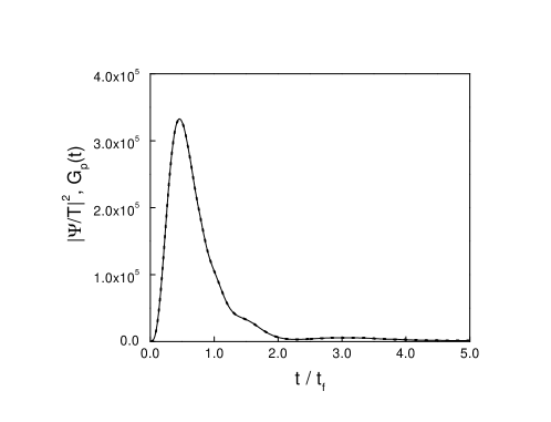
Figure 1: Plot of $|\Psi(d,t)|^{2}$ (solid line) and $G_{\rm p}(t)$ (dotted line) at the barrier edge $x=d=10.083$ nm as a function of time in units of the free passage time $t_{f}$. The time-dependent solution is normalized to the transmission coefficient $|T|^{2}$.

At early times one sees a time-domain resonance structure gcv01 . The maximum of this transient structure represents the largest probability to find the tunneling particle at the barrier edge $x=d$. In our example, as shown in Fig. 1, the maximum of the time-domain resonance occurs at $t_{p}=5.347$ fs, faster than the free passage time across the same distance of $10.083$ nm, that is, $t_{p}/t_{f}=0.455$. From $t/t_{f}=2.0$ onward the probability density approaches essentially to its asymptotic value. We have also included in Fig. 1 the plot of $G_{\rm p}(t)$ (dotted line) calculated from Eq. (4) for the same set of parameters; it is indistinguishable from the previous calculation, i.e., both curves coincide exactly.

V Concluding remarks

We have found a surprising relationship between the real time Feynman histories approach and an analytical expression for the probability density for cutoff initial waves involving the quantum shutter setup for the “passage time” in tunneling. This may prove to be of interest in the pursue of elucidating the notion of tunneling time through a classically forbidden region.

- (1) L. A. MacColl, Phys. Rev. 40, 621 (1932).
- (2) See for example: E. H. Hauge and J. A. Støvneng, Rev. Mod. Phys. 61, 917 (1989); R. Landauer and Th. Martin, Rev. Mod. Phys. 66, 217 (1994); Time in Quantum Mechanics, edited by J. G. Muga, R. Sala, I. L. Egusquiza (Springer-Verlag, Berlin, 2002).
- (3) N. Yamada, Phys. Rev. A 54, 182 (1996).
- (4) N. Yamada, Phys. Rev. Lett. 83, 3350 (1999).
- (5) N. Yamada, (unpublished) (2002); in Meeting Abstracts of the Physical Society of Japan, 55, Issue 2, Part2, 23pWD-3, 227 (2000) (in Japanese).
- (6) G. García-Calderón and A. Rubio, Phys. Rev. A 55, 3361 (1997).
- (7) G. García-Calderón and J. Villavicencio, Phys. Rev. A 64, 012107 (2001).
- (8) R. P. Feynman and A. R. Hibbs, Quantum Mechanics and Path Integrals (McGraw-Hill, New York, 1965).
- (9) Here we consider such a probability distribution of tunneling times that is intrinsic to the scattering event.
- (10) M. Büttiker and R. Landauer, Phys. Rev. Lett 49, 1739 (1982).
- (11) D. G. Sokolovskii and L. M. Baskin, Sov. Phys. Tech. Phys. 30, 1076 (1985).
- (12) L. S. Schulman and R. W. Ziolkowski, in Proceedings of Third International Conference on Path Integrals from meV to MeV, edited by V. Sa-yakanit et al. (World Scientific, Singapore, 1989), p. 253.
- (13) G. García-Calderón and J. Villavicencio, Preprint arXiv: quant-ph/0008014 (2000).
- (14) M. Gell-Mann and J. B. Hartle, in Proceedings of the 3rd International Symposium on the Foundations of Quantum Mechanics in the Light of New Technology, edited by S. Kobayashi et al. (Physical Society of Japan, Tokyo, 1990), p. 321.
- (15) M. Gell-Mann and J. B. Hartle, in Proceedings of the 25th International Conference on High Energy Physics, edited by K. K. Phua and Y. Yamaguchi (World Scientific, Singapore, 1991), p. 1303.
- (16) J. B. Hartle, Phys. Rev. D 44, 3173 (1991); M. Gell-Mann and J. B. Hartle, Phys. Rev. D 47, 3345 (1993).
- (17) J. Humblet and L. Rosenfeld, Nucl. Phys. 26, 529 (1961).
- (18) V. N. Faddeyeva and N. M. Terent’ev, Tables of values of the function for complex argument, translated from the Russian by D. G. Fry and B. A. Hons (Pergamon, London, 1961); Handbook of Mathematical Functions, edited by M. Abramowitz and I. A. Stegun (Dover, New York, 1965), p. 297; G. P. M. Poppe and C. M. J. Wijers, ACM Transactions on Mathematical Software, 16, 38 (1990); 16, 47 (1990). The above references discuss also numerical methods to evaluate the complex error function .
- (19) E. C. Tichmarsh, The Theory of Functions (Oxford University Press, London, 1939), 2nd ed., p. 110.
- (20) G. García-Calderón (unpublished). A similar expansion in 3 dimensions is presented in the paper, G. García Calderón and A. Rubio, Nucl. Phys. A 458, 560 (1986).
- (21) G. García-Calderón, Solid State Commun. 62, 441(1987).
- (22) D. K. Ferry and S. M. Goodnick, Transport in Nanostructures (Cambridge University Press, United Kingdom, 1997), pp. 91-201.