Decoherence in Discrete Quantum Walks

Abstract

We present an introduction to coined quantum walks on regular graphs, which have been developed in the past few years as an alternative to quantum Fourier transforms for underpinning algorithms for quantum computation. We then describe our results on the effects of decoherence on these quantum walks on a line, cycle and hypercube. We find high sensitivity to decoherence, increasing with the number of steps in the walk, as the particle is becoming more delocalised with each step. However, the effect of a small amount of decoherence can be to enhance the properties of the quantum walk that are desirable for the development of quantum algorithms, such as fast mixing times to uniform distributions.

1 Introduction to Quantum Walks

Quantum walks are based on a generalisation of classical random walks, which have found many applications in the field of computing. Examples of the power of classical random walks to solve hard problems include algorithms for solving $k$-SAT Schöning [1999], estimating the volume of a convex body Dyer et al. [1991], and approximation of the permanent Jerrum et al. [2001]. They are a subset of a wider model of computation, cellular automata, which have been proved universal for classical computation. The utility of classical walks suggests that extending the formalism to the quantum regime may assist the new field of quantum information processing in generating further quantum algorithms. Similarly to the classical case, it is also possible to define the notion of quantum cellular automata, whose equivalence to quantum Turing machines has been shown Watrous [1995].

Most known quantum algorithms are based on the quantum Fourier transform, for an introduction to quantum computing and algorithms see, e. g., Shor [2000], Nielsen and Chuang [2000]. Quantum versions of random walks provide a distinctly different paradigm in which to develop quantum algorithms. Very recently, two such algorithms have been presented. Shenvi et al. Shenvi et al. [2002] proved that a quantum walk can perform the same task as Grover’s search algorithm Grover [1996], with the same quadratic speed up. Childs et al. Childs et al. [2002] describe a quantum algorithm for transversing a particular graph exponentially faster than can be done classically. This exponential speed up is very promising, though the problem presented is somewhat contrived.

In fact, several possible extensions of classical random walks to the quantum regime have been proposed Farhi and Gutmann [1998], Childs et al. [2001], Grossing and Zeilinger [1988], however, here we will only treat the discrete time, coined quantum walks Aharanov et al. [2001], subsequently these are referred to simply as “quantum walks”. Before introducing quantum walks, it is helpful to review the properties of classical random walks. This is followed by an overview of quantum walks on a line, $N$-cycle, and hypercube. Section 2 presents our results on the effects of decoherence in these quantum walks.

1.1 Classical Random Walks on Graphs

The discrete space on which a random walk takes place can most generally be described as a graph $G(V,E)$ with two components, a set of vertices $V$, and a set of edges $E$. An edge may be specified by the pair of vertices that it connects, $e=(v_{i},v_{o})$. The graph is undirected when $(v_{i},v_{o})\in E~{}{\text{iff}}(v_{o},v_{i})\in E$. The second essential feature of a classical walk is the (time-independent) transition matrix $M$, whose elements $M_{ij}$ provide the probability for a transition from vertex $v_{i}$ to vertex $v_{j}$. These probabilities are non-zero only for a pair of vertices connected by an edge,

$$M_{ij}\neq 0\mbox{\hskip 10.00002pt iff \hskip 4.30554pt}e=(v_{i},v_{j})\in E\;.$$ (1)

The walk is unbiased if the non-zero elements of $M$ are given by $M_{ij}=\frac{1}{d_{i}}$, where $d_{i}$ is the degree of the vertex $v_{i}$ (the number of edges connected to $v_{i}$). A graph is called regular ($d$-regular) if all vertices have equal degree ($d$). The state of a classical random walk at a given time $t$ is described by a probability distribution $P(v,t)$ over the vertices $v\in V$. This distribution evolves at each time step by application of the transition matrix $M$,

$$P(v,t)=M^{t}P(v,0)\;.$$ (2)

A number of features of these classical walks are worthy of note for later comparisons. If $G$ is connected (every pair of vertices have a path linking them via a sequence of edges), then the walk tends to a steady state distribution $\pi$ which is independent of the initial state $P(v,0)$. Further, if the graph is regular then the limiting distribution is uniform on all the vertices. An exception arises in the case of periodic random walks, however, a “resting probability” for the walk to remain at the current vertex may be added which breaks the periodicity and restores the usual convergence. The rate of convergence to this limiting distribution may described in a number of ways, here we choose the mixing time,

$$M_{\varepsilon}^{\mathrm{C}}=\min\left\{T|\forall t>T:||P(v,t)-\pi||_{\text{tv}}<\varepsilon\right\}\;.$$ (3)

The measure used here is the total variational distance,

$$||p_{1}-p_{2}||_{\text{tv}}=\sum_{v_{i}\in V}|p_{1}(v_{i})-p_{2}(v_{i})|\;.$$ (4)

The mixing time thus gives a measure of the time after which the distribution is within a distance $\varepsilon$ of the limiting distribution and remains at least this close. An alternative measure that is useful in classical algorithms, for example 3-SAT Schöning [1999], is the hitting time. This is defined for a pair of vertices $v_{0}$, $v_{1}$ as the expected time at which a walk starting at $v_{0}$ reaches $v_{1}$ for the first time.

1.2 Criteria for a Quantum Walk

Given a $d$-regular graph, $G(V,E)$, the associated Hilbert space may be defined as

$${\cal H}_{V}={\text{span}}\{\mbox{$|v_{i}\rangle$}\}^{|V|}_{i=1}\;.$$ (5)

As already mentioned, several extensions of classical random walks to the quantum regime have been proposed, there is no unique way to do this. To guide us, we note there are several properties of classical random walks and quantum systems that we would like such quantum walks to have, if possible. The three desirable properties of the classical transition matrix $M$ are,

• locality: $M_{ij}\neq 0~{}{\text{iff}}~{}e=(v_{i},v_{j})\in E$, i. e., transitions are only between vertices directly connected by an edge

• homogeneity: if $e=(v_{i},v_{j})\in E,~{}|M_{ij}|=\frac{1}{d_{i}}$, i. e., equal probability of transition to any neighbouring vertex

• time independence: the current step does not depend in any way on previous steps of the random walk (Markovian)

The quantum transition matrix $U$, equivalent to $M$, should have similar properties to $M$. In addition, it should be

• unitary

because all pure quantum processes are unitary. As proved by Meyer Meyer [1996a, b], this requirement of unitarity is incompatible with the three prior properties, except in very special circumstances that don’t produce interesting quantum dynamics. In order to generate a non-trivial quantum evolution, one or more of these constraints must be relaxed. The continuous time quantum walks proposed by Farhi and Gutmann Farhi and Gutmann [1998], is non-local, in the sense that there is a small probability of the particle moving arbitrarily far away in a given unit time interval. The quantum cellular automata of Meyer Meyer [1996b, c] are not homogeneous, in that the full dynamics is specified over two time steps rather than one. One may make the quantum walk non-unitary by measuring the particle at each step, but this simply reproduces the classical random walk. Finally, one may consider relaxing the time independence condition slightly, and this is what the coined quantum walks effectively do. For completeness, we note that there is an equivalent formulation of the coined quantum walk in terms of a simple quantum process on a directed graph, derived from the original undirected graph, that is due to Watrous Watrous [2001].

1.3 Coined Quantum Walks

By analogy with the classical walk, in which one pictures flipping a coin at each time-step to determine which edge to leave the current vertex by, interesting quantum results may be obtained by the introduction of an explicit (quantum) coin. In addition to the particle, with associated Hilbert space ${\cal H}_{\mathrm{V}}$ as given in (5), there is an auxiliary quantum system, the coin, with a Hilbert space of dimension $d$ (the degree of the graph) ${\cal H}_{\mathrm{C}}=\mathbb{C}^{d}$. The transition matrix is then defined as a unitary matrix $U$ acting on the tensor product of these two spaces. This unitary is constructed from two separate operators, a “coin flip” and a conditional translation. For an unbiased walk, the coin flip operator, $\mathbf{C}$ is a unitary matrix whose elements all have equal modulus in the computational basis of the coin. This adds significant new degrees of freedom to the system, as the relative phases of these elements may be chosen arbitrarily. The conditional translation $\mathbf{T}$ moves the particle along an edge to an adjacent vertex determined by the state of the coin. The evolution of the system from an initial state $\mbox{$|\psi(0)\rangle$}_{\mathrm{CV}}$ to $\mbox{$|\psi(t)\rangle$}_{\mathrm{CV}}$ after $t$ steps is thus given by,

$$\mbox{$|\psi(t)\rangle$}_{\mathrm{CV}}=\left[\mathbf{T}\cdot(\mathbf{C}\otimes\mathbb{I})\right]^{t}\mbox{$|\psi(0)\rangle$}_{\mathrm{CV}}\;.$$ (6)

The coin can also be thought of as forming a $d$-state quantum memory from one step to the next, allowing a much wider range of dynamics to be fully reversible (a necessary property of unitary evolution).

Unitary evolution is also completely deterministic, so the choice of initial condition is never “washed out”, rather, it plays a key role in determining the outcome of the quantum walk. Unitarity also means that the joint state of the coin and particle can never reach a steady state. Even the induced probability distribution over the nodes obtained by tracing out the coin,

$$P(v,t)=~{}_{\mathrm{V}}\mbox{$\langle v|$}{\mathrm{Tr_{C}}}\left[\mbox{$|\psi(t)\rangle$}_{\mathrm{CV}}\mbox{$\langle\psi(t)|$}\right]\mbox{$|v\rangle$}_{\mathrm{V}}\;,$$ (7)

does not converge to a long-time limit. However, it is possible to define a time-averaged probability distribution that does reach a steady state,

$$\overline{P(v,T)}=\sum_{t=0}^{T-1}\frac{P(v,t)}{T}\;.$$ (8)

Operationally, this is easy to produce, it is the distribution obtained by sampling the particle location at some time $t$ uniformly selected at random from $0\leq t<T$. Using this distribution it is possible to define a quantum mixing time similar to that in (3),

$$M_{\varepsilon}^{\mathrm{Q}}=\min\left\{T|\forall t>T:||\overline{P(v,t)}-\pi||_{\text{tv}}<\varepsilon\right\}\;.$$ (9)

The second measure discussed for classical random walks was the hitting time. This can also be extended to quantum walks, but as before will require some modification. In the classical case it is possible to measure the location of the particle at each time step to ascertain whether or not it has reached the desired vertex. The equivalent quantum measurement disturbs the system; if a complete projection onto the vertex Hilbert space is performed at each step then all coherences are lost and a classical distribution results. There are two approaches to this problem that have been used in the literature Kempe [2002]. It would be possible to wait until a chosen time, $T$, and then perform a full measurement over all the vertices. If the probability of being at the desired vertex is greater than some value $p$ which is bounded below by an inverse polynomial in the size of the graph, it is said that the walk has a $(T,p)$ one-shot hitting time. (This lowerr bound ensures that standard amplification procedures can efficiently raise the success probability arbitrarily close to unity.) The second alternative is to perform a partial measurement at each time step. Projecting onto the subspaces given by the desired vertex $v$, $I\!\!P_{v}=\mbox{$|v\rangle$}\mbox{$\langle v|$}$, and its orthogonal complement, $I\!\!P_{\bar{v}}=\mathbb{I}-\mbox{$|v\rangle$}\mbox{$\langle v|$}$ will halt the walk once the vertex $v$ is reached. A walk has a $(T,p)$ concurrent hitting time if $I\!\!P_{v}$ is measured with probability greater or equal to $p$, which again must have as a lower bound an inverse polynomial in the graph size, in a time $T$. Both these quantities have been shown to exhibit an exponential speed up over the classical case for a walk between opposite corners of a hypercube Kempe [2002].

Explicit solution of a quantum walk has proved to be a difficult problem. In certain cases standard techniques from classical graph theory have been applied with some success, namely solution in the Fourier space of the problem Ambainis et al. [2001], Aharanov et al. [2001], and also the technique of generating functions Bach et al. [2002]. Fourier solutions are possible when the graph is of a particular form, known as a Cayley graph. Any discrete group has an associated Cayley graph, in which the elements of the group form the vertices and the edges are placed by choosing a complete set of generators, $g_{i}$ and placing an edge between the vertices $a$ and $b$ iff, $a=g_{i}b$ for one of the $g_{i}$. This produces an undirected graph results if the group is Abelian. We will next consider three specific cases of such graphs for which analytical solution has proved possible.

1.4 Coined Quantum Walk on a Line

Consider the case when the graph consists of an lattice of points at integer positions on an infinite line. The Hilbert space of the particle is represented by the integers,

$${\cal H}_{V}={\text{span}}\{\mbox{$|x\rangle$}:x\in\mathbb{Z}\}\;.$$ (10)

At each time interval the particle can move one step to either the left or the right, the coin thus requires only a two dimensional Hilbert space which can conveniently be written as,

$${\cal H}_{C}=\{\mbox{$|R\rangle$},\mbox{$|L\rangle$}\}\;.$$ (11)

The conditional translation $\mathbf{T}$ thus has the following action on the basis states,

$$\mathbf{T}\mbox{$|R,x\rangle$}=\mbox{$|R,x+1\rangle$}\;,\hskip 21.33955pt\mathbf{T}\mbox{$|L,x\rangle$}=\mbox{$|L,x-1\rangle$}\;.$$ (12)

The evolution of the probability distribution induced on the lattice may now be compared with that of the analogous classical walk on a line. It is sufficient to us the Hadamard operator as the coin flip,

$$\mathbf{H}=\frac{1}{\sqrt{2}}\left(\begin{array}[]{cc}1&1\\ 1&-1\end{array}\right)\;,$$ (13)

all others are essentially equivalent Ambainis et al. [2001], Bach et al. [2002]. We also choose the initial state to be

$$\mbox{$|\psi(0)\rangle$}=\frac{1}{\sqrt{2}}\left(\mbox{$|R\rangle$}+i\mbox{$|L\rangle$}\right)\otimes\mbox{$|0\rangle$}\;.$$ (14)

This choice produces a symmetric distribution, as in the classical case. Since $\mathbf{H}$ and $\mathbf{T}$ contain only real elements, there is no interference between the part of the walk due to the initial state $|R\rangle$ and that due to $i\mbox{$|L\rangle$}$. Thus the natural (in terms of basis states) outcome of a quantum walk is actually biased, unlike a classical random walk, a basic demonstration of the initial condition affecting the entire outcome of the walk.

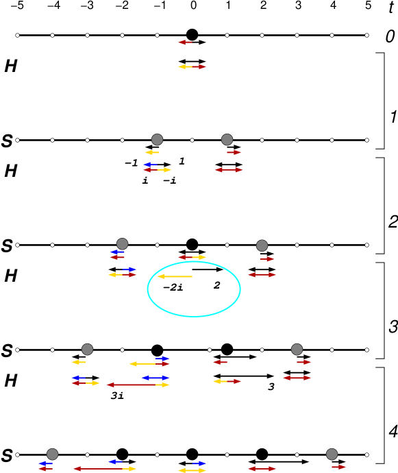
Figure 1: A schematic representation of the first four steps of the evolution of the 1-D walk with a Hadamard coin. Circles show the particle positions and arrows show the state of the coin, with relative magnitudes indicating the amplitude of the components of the wavefunction

Four steps of this evolution are shown schematically in Fig. (1) and the respective probability distributions are shown in Fig. (2) after 100 time steps.

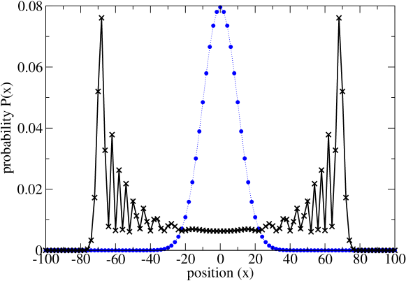
Figure 2: A comparison of the probability distribution of a classical and coined quantum walk on a line, after 100 time steps. Only even points are plotted as both functions are zero on the odd grid points

The classical walk forms a binomial distribution, with a mean of 0 and standard deviation $\sigma_{\mathrm{C}}=\sqrt{T}$. Figure 2 displays several of the interesting features of a quantum walk. The central interval $[-2\sqrt{T},2\sqrt{T}]$ is essentially uniform in the quantum case, with oscillating peaks outside this region up to $[-T/\sqrt{2},T/\sqrt{2}]$. This is due to interference between the large number of possible paths to each point in this range.

The quantum walk on a line has been solved exactly Ambainis et al. [2001], Nayak and Vishwanath [2000] using both real space (path counting) and Fourier space methods. The solutions are complicated, mainly due to the “parity” property, namely, that the solutions must have support only on even(odd)-numbered lattice sites at even(odd) times. The moments can be calculated for asymptotically large times, for a walk starting at the origin, the standard deviation is

$$\lim_{T\rightarrow\infty}\sigma_{\mathrm{Q}}=\left(1-\frac{1}{\sqrt{2}}\right)^{1/2}T\;.$$ (15)

The standard deviation $\sigma_{\mathrm{Q}}$ is thus linear in $T$, in contrast to $\sqrt{T}$ for the classical walk.

Quantum walks on a line have now been studied in considerable detail. Discussions of absorbing boundaries have been given Bach et al. [2002], Yamasaki et al. [2002], Ambainis et al. [2001], with applications to halting problems in mind. Extensions to multiple coins have been made by Brun et al. Brun et al. [2002a, b]. However, though useful for understanding the basic properties of quantum walks, the walk on a line is too simple to yield interesting quantum problems for significant algorithms.

1.5 Coined Quantum Walk on a $N$-Cycle

If periodic boundary conditions are applied, instead of a walk on an infinite line, a closed walk on a $N$-cycle is obtained. For this system, which wraps round on itself, the standard deviation is inappropriate and mixing times must be considered. The classical result is well known,

$$\overline{M}_{\varepsilon}^{\mathrm{C}}=o(N^{2}/\varepsilon)\;.$$ (16)

Here the time average of the probability distribution, $\overline{P(v,T)}$ has been used in (3) for ease of comparison with the quantum case. The usual mixing time defined by (3) using $P(v,T)$ scales as $M_{\varepsilon}^{\mathrm{C}}=o(N^{2}\log(1/\varepsilon))$. The scaling of $\varepsilon$ is not important for the quantum–classical comparisons we will do here, more details can be found in Aharanov et al. [2001]. The equivalent quantity for a quantum walk was bounded above by Aharonov et al. Aharanov et al. [2001], and shows a quadratic speed-up,

$$M_{\varepsilon}^{\mathrm{Q}}\leq O\left(\frac{N\log N}{\varepsilon^{3}}\right)\;.$$ (17)

Bounds have also been established in the case of more general graphs and it is conjectured that mixing times can be improved at most polynomially by quantum walks Aharanov et al. [2001]. Numerical studies, see Kendon and Tregenna [2003], suggest the form of the quantum mixing time is actually $M_{\varepsilon}^{\mathrm{Q}}=O\left(N/\varepsilon\right)$, and explain why tighter analytical bounds are hard to obtain.

1.6 Coined Quantum Walk on a Hypercube

A hypercube of dimension $N$ is a Cayley graph with $2^{N}$ vertices labelled by the bit-strings of length $N$. The Hilbert space for this graph is spanned by the basis states $\mbox{$|x\rangle$},\,x\in[0,2^{N}]$. Each vertex has degree $N$, so the state space of the coin is $\mathcal{H}_{\mathrm{C}}=\mathbb{C}^{N}$. The basis vectors of this space are denoted by $\mbox{$|a\rangle$},\,a\in[0,N]$. These states correspond to the $N$ vectors $|e_{a}\rangle$ where $e_{a}$ is the vector with all zeroes except for a single one in the $a^{\text{th}}$ position. The translation operator for the walk on a hypercube can then be defined as,

$$\mathbf{T}\mbox{$|a,x\rangle$}=\mbox{$|a,x\oplus e_{a}\rangle$}\;.$$ (18)

Any $N\times N$ unitary matrix with all elements of unit modulus may be used as an unbiased coin, however, this is not the most natural choice given the symmetries of the hypercube. Instead, a biased coin has been selected, which distinguishes the edge along which the particle arrived at the vertex from all the others Moore and Russell [2001]. This “Grover” coin acts thus,

$$\mathbf{G}\mbox{$|a\rangle$}=\frac{2}{N}\sum_{b}\mbox{$|b\rangle$}-\mbox{$|a\rangle$}\;.$$ (19)

The full evolution for a single time step of this walk is then given by $\mathbf{U}=\mathbf{T}\cdot(\mathbf{G}\otimes\mathbb{I})$.

The quantum walk on the hypercube can be solved analytically by mapping it to a walk on a line with a variable coin operator, provided the symmetry of the hypercube is maintained throughout. To preserve the symmetry between particle states with equal Hamming weights, defined to be the number of 1’s in their bit-string, the initial state must be chosen to be localised on the hypercube at $|0\rangle$ with the coin in an equal superposition of all its states, $\mbox{$|\psi(0)\rangle$}=\tfrac{1}{\sqrt{N}}\sum_{a}\mbox{$|a\rangle$}\otimes\mbox{$|0\rangle$}$. With this ansatz it has been shown by Moore and Russell Moore and Russell [2001] that the walk has an exact instantaneous mixing time, when the distribution transiently becomes exactly uniform, at $T=\pi N/4$. More importantly, Kempe Kempe [2002] found the first exponential gap between classical and quantum walks for hitting times on the hypercube. Both the concurrent and one-shot hitting times for a walk to travel from $|0\rangle$ to $|2^{N}\rangle$ are found to be $\pi N/2$, with small error probability. This is exponentially faster than the classical hitting time, $T=2^{N-1}$. This is not a true quantum speed up, since there are more sophisticated classical algorithms than a random walk to reach the opposite corner that exploit the symmetry of the hypercube. Nonetheless, it is important as the first indication that quantum walks have the potential for driving quantum algorithms with exponentially faster, later confirmed by Childs et al. Childs et al. [2002] on a more random graph.

2 Decoherence in Quantum Walks

We will now study each of the three systems just introduced in the presence of decoherence. A simple model of decoherence is chosen here, at each time step of the quantum walk a measurement is made in the computational basis with a probability $p$. We consider three cases, where the measurement is over only the coin degrees of freedom, only over the particle states, or is a complete measurement of both. Given a unitary transform $\mathbf{U}=\mathbf{T}\cdot(\mathbf{C}\otimes\mathbb{I})$ for each step of the walk as described by (6), the effect of this decoherence model can be described as a discrete master equation,

$$\varrho(t+1)=(1-p)U\varrho(t)U^{\dagger}+p\sum_{i}I\!\!P_{i}U\varrho(t)U^{\dagger}I\!\!P_{i}\;.$$ (20)

The summation runs over the dimensions of the Hilbert space on which the decoherence occurs, either the coin $\mathcal{H}_{C}$, the particle $\mathcal{H}_{V}$ or both $\mathcal{H}_{C}\otimes\mathcal{H}_{V}$. The projectors $I\!\!P_{i}$ are defined to act in the computational basis. When $p=0$ the ideal quantum walk is obtained, and for $p=1$ when a measurement is made at each time step it produces the classical random walk.

The numerical work summarised in the remainder of this paper has been presented more fully in Kendon and Tregenna [2003].

2.1 Decoherence in a Quantum Walk on a Line

Since there is an experimental proposal to implement a quantum walk on a line in an optical lattice Dür et al. [2002], as well as the three examples for $I\!\!P_{i}$ given above, we considered the likely form of experimental errors, and also modeled the effect of an imperfect Hadamard on the coin. The Hadamard operation may be considered to be a “rotation” about the computational basis by $\pi/4$, (actually a rotation and reflection since $\det(\mathbf{Rot}(\theta))=-1$),

$$\mathbf{Rot}(\theta)=\left(\begin{array}[]{cc}\sin(\theta)&\cos(\theta)\\ \cos(\theta)&-\sin(\theta)\end{array}\right)\;,$$ (21)

The error model used in this case consisted of a Gaussian spread of standard deviation $\sqrt{p}\pi/4$ about the ideal value of $\theta=\pi/4$.

All types of decoherence model produce the same general form for the decay of $\sigma_{p}(T)$ from the quantum to the classical value, with small differences in the rates, as shown in Fig. 3.

Figure 3: Standard deviation $\sigma_{p}(T)$ of the particle on a line for different models of decoherence, for $T=100$ time steps

The slope of $\sigma_{p}(T)$ is finite as $p\rightarrow 0$ and zero at $p=1$. We have calculated $\sigma_{p}(T)$ analytically for $pT\ll 1$ and $T\gg 1$ for the case where $I\!\!P_{i}$ is the projector onto the preferred basis $\{\mbox{$|a,x\rangle$}\}$, i. e., the decoherence affecting both particle and coin. Details are given in Kendon and Tregenna [2002]), the result is

$$\sigma_{p}(T)\leq\sigma(T)\left[1-\frac{pT}{6\sqrt{2}}+\frac{p}{\sqrt{2}}(1-1/\sqrt{2})+O(p^{2},1/T)\right]\;.$$ (22)

The first order dependence is thus proportional to $pT$, so the sensitivity to decoherence grows linearly in $T$ for a given decoherence rate $p$.

There are interesting differences in the shape of the distribution of the particle position for each of the types of decoherence. The decoherence rate that gives the closest to uniform distribution has been selected and plotted in Fig. 4, along with the pure quantum and classical distributions for comparison.

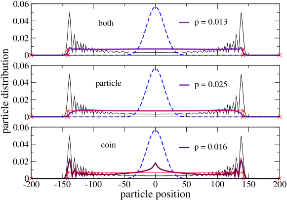
Figure 4: Distribution of the particle position for a quantum walk on a line after $T=200$ time steps. Pure quantum (dotted), fully classical(dashed), and decoherence at rate shown on part of system indicated by key (solid). Uniform distribution between $-T/\sqrt{2}\leq x\leq T/\sqrt{2}$ (crosses) also shown

When the particle position is subject to decoherence that tends to localise the particle in the standard basis, this produces a highly uniform distribution between $\pm T/\sqrt{2}$ for a particular choice of $p$. The optimal decoherence rate $p_{u}$ can be obtained by minimising the total variational distance between the actual and uniform distributions,

$$\nu(p,T)\equiv||P(x,p,T)-P_{u}(T)||_{\text{tv}}\equiv\sum_{x}|P(x,p,T)-P_{u}(T)|\;,$$ (23)

where $P(x,p,T)$ is the probability of finding the particle at position $x$ after $T$ time steps, regardless of coin state [compare (7)], and $P_{u}(T)=\sqrt{2}/T$ for $-T/\sqrt{2}\leq x\leq T/\sqrt{2}$ and zero otherwise. The optimum decoherence rate depends on the number of steps in the walk, it can be determined numerically that $p_{u}T\simeq 2.6$ for decoherence on both the particle and the coin, and $p_{u}T\simeq 5$ for decoherence on the particle only. These differences in the quality of the uniform distribution are independent of $p$ and $T$, and provide an order of magnitude (0.6 down to 0.06) improvement in $\nu$ over the pure quantum value. Decoherence just on the coin does not enhance the uniformity of the distribution, as Fig. 4 shows, there is a cusp at $x=0$.

2.2 Decoherence in a Quantum Walk on a $N$-Cycle

We now consider a walk on a $N$-cycle subjected to decoherence. There is an experimental proposal for implementation of a quantum walk on a cycle in the phase of a cavity field Sanders et al. [2002], in which further aspects of decoherence in such quantum walks are considered. Recall from Sect. 1.5 that the pure quantum walk on a cycle with $N$ odd, is known Aharanov et al. [2001] to mix in time $\leq O(N\log N)$ if a Hadamard coin is used. The quantum walk on a cycle with $N$ even does not mix to the uniform distribution with a Hadamard coin, but can be made to do so by appropriate choice of coin flip operator Tregenna et al. [2003]. Under the action of a small amount of decoherence, the mixing time becomes shorter for all cases, typical results are shown in Fig. 5. In particular, decoherence causes the even-$N$ cycle to mix to the uniform distribution even when a Hadamard coin is used.

Figure 5: Numerical data for mixing times on cycles of size $N=29$ and $N=30$ ($\square$), for coin (dotted), particle (dashed) and both (solid) subject to decoherence, using $\varepsilon=0.01$. Also $N=28$ ($\times$) for coin. Both axes logarithmic

The asymptotes in Fig. 5 for $N$ even and decoherence on the coin only, for $p<2/N$, are well fitted by $\varepsilon pM_{\varepsilon}\simeq N/4$ for $N$ divisible by 2, and $\varepsilon pM_{\varepsilon}\simeq N/16$ for $N$ divisible by 4. For larger $p$, the mixing time tends to the classical value of $N^{2}/16\varepsilon$. Although for $N$ divisible by 4, the (coin-decohered) mixing time shows a minimum below the classical value at $p\simeq 2/N$, this mixing time is still quadratic in $N$. Thus although noise on the coin causes the even-$N$ cycle to mix to the uniform distribution, it does not produce a significant speed up over the classical random walk.

For decoherence on the particle position, with $p<16/N^{2}$, $\varepsilon pM_{\varepsilon}\simeq 1/(N/2-1)$ for $N$ divisible by 2, and $\varepsilon pM_{\varepsilon}\simeq 1/(N/4+3)$ for $N$ divisible by 4. At $p\simeq 16/N^{2}$, there is a minimum in the mixing time at a value roughly equal to the $(N+1)$-cycle pure quantum mixing time, $M^{(\text{min})}_{\varepsilon}\sim\alpha N/\varepsilon$ (with $\alpha$ a constant of order unity). Decoherence on the particle position thus causes the even-$N$ cycle to mix in linear time for a suitable choice of decoherence rate $p^{(\text{min})}\sim 16/N^{2}$, independent of $\varepsilon$ so long as $\varepsilon<1/N$.

For all types of decoherence, the odd-$N$ cycle shows a minimum mixing time at a position somewhat earlier than the even-$N$ cycle, roughly $p=2/N^{2}$, but because of the oscillatory nature of $\overline{P(x,p,T)}$, the exact behaviour Kendon and Tregenna [2003] is not a smooth function of $p$ or $\varepsilon$. As decoherence on the particle (or both) increases, at $p\simeq 16/N^{2}$, the mixing time passes through an inflexion and from then on behaves in a quantitatively similar manner to the adjacent-sized even-$N$ cycles, including scaling as $M^{(\text{min})}_{\varepsilon}\sim\alpha N/\varepsilon$ at the inflexion. Thus for at least $0\leq p\lesssim 16/N^{2}$ the mixing time stays linear in $N$, and exhibits the quantum speed up over the classical $N^{2}$.

2.3 Decoherence in a Quantum Walk on a Hypercube

Recalling from Sect. 1.6, we are interested in the hitting time to the opposite corner, which was shown by Kempe Kempe [2002] to be polynomial, an exponential speed up over a classical random walk. Kempe discusses two types of hitting times, one-shot, where a measurement is made after a pre-determined number of steps, and concurrent, where the desired location is monitored continuously to see if the particle has arrived. In each case, the key parameter is the probability $P_{h}$ of finding the particle at the chosen location. Here we consider only target locations exactly opposite the starting vertex. We have calculated $P_{h}$ numerically following the scheme of Moore and Russell [2001], Kempe [2002] with a $N$-dimensional coin and the Grover coin operator, defined in (19).

Figure 6: Hitting probability on a 9–dimensional hypercube for one-shot (left) and concurrent (right), perfect walk (circles),with $p=0.05$ (dotted), $p=0.1\simeq 1/9$ (solid). Classical hitting probability barely visible (dashed)

Figure 6 shows how $P_{h}$ is affected by decoherence. All forms of decoherence have a similar effect on $P_{h}$, reducing the peaks and smoothing out the troughs. For the one-shot hitting time this is useful, raising $P_{h}$ in the trough to well above the classical value, so it is no longer necessary to know exactly when to measure. For $p\lesssim 1/N$, the height of the first peak scales as $P_{h}(p)=P_{h}(0)\exp\{-(N+\alpha)p\}$, where $0\lesssim\alpha\lesssim 2$ depending on whether coin, particle or both are subject to decoherence. Thus $P_{h}$ decreases exponentially in $p$, but $p\simeq 1/N$ only lowers $P_{h}$ by a factor of $1/e$, still exponentially better than classical. Continuous monitoring of the target location as in the concurrent hitting time is already a type of controlled decoherence, no new features are produced by the addition of unselective decoherence, but there is still a range of $0<p\lesssim 1/N$ within which the quantum speed up is preserved.

2.4 Summary of Decoherence Effects in Coined Quantum Walks

For the walk on a line, whilst the effect of decoherence is to reduce the standard deviation rapidly towards the classical value, it is possible to generate highly uniform distributions over a range proportional to $T$ for small values of the decoherence parameter, $p$. Uniform sampling is one of the basic tasks for which classical random walks are used, so being able to do this over a quadratically larger range with a quantum walk is certainly promising, though no quantum algorithms using this have been described to date. For a walk on a cycle the effects of decoherence are more beneficial. An optimum rate of decoherence exists for which the rate of mixing is enhanced beyond the pure quantum bound. Further, any amount of decoherence removes the effect of the coin flip operator on the steady state, allowing all such walks to converge to a uniform distribution. Fast mixing to a uniform distribution is again an important basic property required for efficient random sampling, and is the limiting factor in many classical algorithms. For a hypercube, decoherence can still be tolerated so long its rate is kept smaller than $O(1/N)$, which is logarithmic in the system size ($2^{N}$).

Thus, for both experiments and algorithms, decoherence need only be controlled down to finite low levels, rather than negligible levels, in order to observe the intriguing quantum effects displayed by coined quantum walks. Many open problems remain concerning the best ways to do this, how to exploit the full power of the extra degrees of freedom provided by the quantum coin, and how to make quantum walks perform useful tasks over more general graphs that provide real quantum computational advantages over classical algorithms.

References

- Schöning [1999] U Schöning. A probabilistic algorithm for k-SAT and constraint satisfaction problems. In 40th Annual Symposium on Found. of Comp. Sci., pages 17–19. IEEE, 1999.
- Dyer et al. [1991] M Dyer, A Frieze, and R Kannan. A random polynomial-time algorithm for approximating the volume of convex bodies. J. of the ACM, 38(1):1–17, 1991.
- Jerrum et al. [2001] M Jerrum, A Sinclair, and E Vigoda. A polynomial-time approximation algorithm for the permanent of a matrix with non-negative entries. In Proc. 33rd STOC, pages 712–721. Assoc. for Comp. Machinery, New York, 2001.
- Watrous [1995] J Watrous. In Proc. 36th Ann. Symp. on Foundations of Computer Science, pages 528–537. Assoc. for Comp. Machinery, New York, 1995.
- Nielsen and Chuang [2000] M A Nielsen and I J Chuang. Quantum Computation and Quantum Information. Cambridge University Press, Cambs. UK, 2000.
- Shor [2000] Peter W. Shor. Introduction to quantum algorithms. quant-ph/0005003, 2000.
- Shenvi et al. [2002] Neil Shenvi, Julia Kempe, and K Birgitta Whaley. A quantum random walk search algorithm. Phys. Rev. A, 2002. quant-ph/0210064, to appear.
- Grover [1996] L K Grover. A fast quantum mechanical algorithm for database search. In Proc of the 28th Annual STOC, pages 212–219. Assoc. for Comp. Machinery, New York, 1996.
- Childs et al. [2002] A M Childs, Richard Cleve, Enrico Deotto, Edward Farhi, Sam Gutmann, and Daniel A Spielman. Exponential algorithmic speedup by quantum walk. quant-ph/0209131, 2002.
- Farhi and Gutmann [1998] E Farhi and S Gutmann. Quantum computation and decison trees. Phys. Rev. A, 58:915–928, 1998. quant-ph/9706062.
- Childs et al. [2001] A M Childs, E Farhi, and S Gutmann. An example of the difference between quantum and classical random walks. quant-ph/0103020, 2001.
- Grossing and Zeilinger [1988] G Grossing and A Zeilinger. Quantum cellular automata. Complex Systems, 2(197-208), 1988.
- Aharanov et al. [2001] D Aharanov, A Ambainis, J Kempe, and U Vazirani. Quantum walks on graphs. In Proc. 33rd STOC, pages 50–59. Assoc. for Comp. Machinery, New York, 2001. quant-ph/0012090.
- Meyer [1996a] D A Meyer. On the absense of homogeneous scalar unitary cellular automata. Phys. Lett. A, pages 337–340, 1996a. quant-ph/9605023.
- Meyer [1996b] D A Meyer. Unitarity in one dimensional nonlinear quantum cellular automata. quant-ph/9605023, 1996b.
- Meyer [1996c] D A Meyer. From quantum cellular automata to quantum lattice gases. J. Stat. Phys., 85(551-574), 1996c. quant-ph/9604003.
- Watrous [2001] J Watrous. Quantum simulations of classical random walks and undirected graph connectivity. J. Comp. System Sciences, 62(2):376–391, 2001. cs.CC/9812012.
- Kempe [2002] Julia Kempe. Quantum random walks hit exponentially faster. quant-ph/0205083, 2002.
- Ambainis et al. [2001] Andris Ambainis, Eric Bach, Ashwin Nayak, Ashvin Vishwanath, and John Watrous. One-dimensional quantum walks. In Proc. 33rd STOC, pages 60–69. Assoc. for Comp. Machinery, New York, 2001.
- Bach et al. [2002] Eric Bach, Susan Coppersmith, Marcel Paz Goldschen, Robert Joynt, and John Watrous. One-dimensional quantm walks with absorbing boundaries. quant-ph/0207008, 2002.
- Nayak and Vishwanath [2000] A Nayak and A Vishwanath. Quantum walk on the line. quant-ph/0010117, 2000.
- Yamasaki et al. [2002] T. Yamasaki, H. Kobayashi, and H. Imai. An analysis of absorbing times of quantum walks. In C. Calude, M. J. Dinneen, and F. Peper, editors, Unconventional Models of Computation, Third International Conference, UMC 2002, Kobe, Japan, October 15-19, 2002, Proceedings, volume 2509 of Lecture Notes in Computer Science, pages 315–330. Springer, 2002. ISBN 3-540-44311-8. quant-ph/0205045.
- Brun et al. [2002a] Todd A Brun, H A Carteret, and Andris Ambainis. The quantum to classical transition for random walks. Phys. Rev. Lett., 2002a. quant-ph/0208195, to appear.
- Brun et al. [2002b] Todd A Brun, H A Carteret, and Andris Ambainis. Quantum random walks with decoherent coins. quant-ph/0210180, 2002b.
- Kendon and Tregenna [2003] Viv Kendon and Ben Tregenna. Decoherence is useful in quantum walks. Phys. Rev. A, 2003. quant-ph/0209005, to appear.
- Moore and Russell [2001] Christopher Moore and Alexander Russell. Quantum walks on the hypercube. quant-ph/0104137, 2001.
- Dür et al. [2002] W Dür, R Raussendorf, H-J Briegel, and V M Kendon. Quantum random walks in optical lattices. Phys. Rev. A, 66:05231, 2002. quant-ph/0207137.
- Kendon and Tregenna [2002] Viv Kendon and Ben Tregenna. Decoherence in a quantum walk on the line. In Quantum Communication, Measurement & Computing (QCMC’02). Rinton Press, 2002. quant-ph/0210047.
- Sanders et al. [2002] Barry Sanders, Steve Bartlett, Ben Tregenna, and Peter L Knight. Quantum quincunx in cavity QED. Phys. Rev. A, 2002. quant-ph/0207028, to appear.
- Tregenna et al. [2003] Ben Tregenna, Will Flanagan, Rik Maile, and Viv Kendon. Tuning quantum walks: coins and initial states. In preparation, 2003.