An efficient scheme for numerical simulations of the spin-bath decoherence

Abstract

We demonstrate that the Chebyshev expansion method is a very efficient numerical tool for studying spin-bath decoherence of quantum systems. We consider two typical problems arising in studying decoherence of quantum systems consisting of few coupled spins: (i) determining the pointer states of the system, and (ii) determining the temporal decay of quantum oscillations. As our results demonstrate, for determining the pointer states, the Chebyshev-based schemeis at least a factor of 8 faster than existing algorithms based on the Suzuki-Trotter decomposition. For the problems of second type, the Chebyshev-based approach has been 3–4 times faster than the Suzuki-Trotter-based schemes. This conclusion holds qualitatively for a wide spectrum of systems, with different spin baths and different Hamiltonians.

I Introduction

Recently, a great deal of attention has been devoted to the study of quantum computation 1 ; 2 . For many physical systems, basic quantum operations needed for implementation of quantum gates have been demonstrated. To be practical, a quantum computer should contain a large number of qubits (some estimates give up to 10⁶ qubits 8 ), and be able to perform many hundreds of quantum gate operations. However, these requirements are not easy to satisfy in experiments. A real two-state quantum system is different from the ideal qubit. The system interacts with its environment, and this leads to a loss of phase relations between different states of the quantum computer (decoherence) 9 ; 9a ; 10 ; 11 , causing rapid accumulation of errors. Detailed theoretical understanding of the decoherence process is needed to prevent this.

More generally, decoherence is an interesting many-body quantum phenomenon which is fundamental for many areas of quantum mechanics, quantum measurement theory, etc 9 ; 9a . It also plays an important role in solid state systems, and might suppress quantum tunneling of defects in crystals 11 , spin tunneling in magnetic molecules and nanoparticles qtm94 ; keiji , or destroy Kondo effect in a dissipationless manner kondo . I.e., decoherence in many physical systems can have experimentally detectable (and sometimes considerable) consequences, and extensive theoretical studies of decoherence are needed to understand behavior of these systems.

Formally speaking, decoherence is a dynamical development of quantum correlations (entanglement) between the central system and its environment. Let us assume that initially the central system is in the state $|\psi_{0}\rangle$ and the environment is in the state $|\chi_{0}\rangle$, so that the state of the compound system (central system plus bath) is $|\Psi(t=0)\rangle=|\psi_{0}\rangle\otimes|\chi_{0}\rangle$. In the course of dynamical evolution, the direct product structure of the state $|\Psi(t)\rangle$ is no longer conserved. If we need to study only the properties of the central system, we can consider the reduced density matrix of the central system, i.e. the matrix $\rho_{S}(t)=\mathop{\rm Tr}_{B}|\Psi(t)\rangle\langle\Psi(t)|$, where $\mathop{\rm Tr}_{B}$ means tracing over the environmental degrees of freedom. Initially, $\rho_{S}(0)=|\psi_{0}\rangle\langle\psi_{0}|$, the system is in pure state, and its density matrix is a projector, i.e. $\rho^{2}_{S}(0)=\rho_{S}(0)$. At $t>0$, this property is lost, and the system appears in a mixed state. It has been shown that, even for relatively small integrable and non-integrable systems, the mixing is sufficient for the time-averaged, quantum dynamical properties of the subsystem to agree with their statistical mechanics values keiji2 . Diagonalizing the density matrix $\rho_{S}$, we can find the (instantaneous) states of the system $|q_{i}(t)\rangle$ and (instantaneous) occupation numbers of these states $w_{i}(t)$. It is generally assumed (and is true for all cases we know) that in “regular” situations, the states $|q_{i}(t)\rangle$ quickly relax to some limiting states $|p_{i}\rangle$, called “pointer states”. This process (decoherence) is, in most cases, much faster than the relaxation of the occupation numbers $w_{i}(t)$ to their limiting values (which correspond to thermal equilibrium of the system with the bath).

The theoretical description of decoherence, i.e. a description of the evolution of the central system from its initial pure state $\psi_{0}$ to the final mixed state, and finding the final pointer states $|p_{i}\rangle$, is a very difficult problem of quantum many-body theory. Some simple models can be solved analytically, for some more complex models different approximations can be employed, such as the Markov approximation for the bath, which assumes that the memory effects in the bath dynamics are negligible. A special case of environment consisting of uncoupled oscillators, so-called “boson bath”, is also rather well understood theoretically. But, although the model of boson bath is applicable for description of a large number of possible types of environments (phonons, photons, conduction electrons, etc.) 11 , it is not universal.

A particularly important case where the boson bath description is inapplicable is the decoherence caused by an enviroment made of spins, e.g. nuclear spins, or impurity spins (so called “spin bath” environment). Similarly, decoherence caused by some other types of quantum two-level systems can be described in terms of the spin bath. Analytical studies of the spin-bath decoherence are difficult, and the spin-bath decoherence of many-body systems is practically unexplored yet. In this situation, numerical modeling of spin-bath decoherence becomes an invaluable research tool.

The most direct approach to study spin-bath decoherence is to compute the dynamical evolution of the whole compound system by directly solving the time-dependent Schrödinger equation of the model system. Even for a modest amount of spins, say 20, such calculations require considerable computational resources, in particular because to study decoherence we have to follow the dynamical evolution of the system over substantial periods of time. Therefore it is worthwhile to explore ways to significantly improve the efficiency of these simulations.

In this paper, we apply the Chebyshev’s expansion method to simulate models for the spin-bath decoherence. This method has been widely applied before TAL-EZER0 ; TAL-EZER ; LEFOR ; kosloff1 ; Iitaka01 ; SILVER ; LOH to study dynamics of large quantum systems, but, to our knowledge, has never been used for simulations of systems made of large number of coupled quantum spins. We show that for realistic problems and typical values of parameters this method is a very efficient tool, giving significant increase in the simulations speed, sometimes up to a factor of eight, in comparison with the algorithms hdr ; hdr1 based on Suzuki-Trotter decompositions SUZUKI1 . We illustrate this point by test examples that we have encountered in our previous studies of the dynamics of the spin-bath decoherence. We also briefly discuss two other approaches, the short iterative Lanczos (SIL) method LEFOR ; sil ; jaklic and the multi-configurational time-dependent Hartree (MCTDH) mctdh1 ; mctdh2 ; mctdh3 method, which are known to demonstrate very good performance in many problems of quantum chemistry.

The remainder of the paper is organized as follows. In Section II, we describe the model and the approaches used for the decoherence simulations. In Section III, we describe the specific details of application of the Chebyshev’s expansion method to the spin-bath decoherence simulations. In Section IV, we present the results of our test simulations. A brief summary is given in the Section V.

II Simulations of the spin-bath decoherence: the model and numerical approaches

We focus on decoherence in quantum systems of several coupled spins. This type of quantum systems is of particular interest for quantum computations, since a qubit can be represented as a quantum spin 1/2, and qubit-based quantum computation is, in fact, a controlled dynamics of the system made of many spins 1/2. Such systems are also of primary interest for studying many solid state problems, since an electron is a particle with the spin 1/2, and its orbital degrees of freedom are often irrelevant. Thus, a system made of several coupled spins 1/2 is a good model for investigating a large class of important problems both in quantum computing, and in solid state theory. The approach described below can be easily extended to arbitrary spin values, but discussion of simulations with arbitrary spins is beyond the scope of this paper.

We consider the following class of models. There is a central system made of $M$ coupled spins ${\bf S}_{m}$ ($S_{m}=1/2$, $m=1\dots M$). The spins ${\bf S}_{m}$ interact with a bath consisting of $N$ environmental spins ${\bf I}_{n}$ ($I_{n}=1/2$, $n=1\dots N$). The Hamiltonian governing behavior of the whole “compound” system (central spins ${\bf S}_{m}$ plus the bath spins ${\bf I}_{n}$) is

$${\cal H}={\cal H}_{0}+{\cal V}={\cal H}_{S}+{\cal H}_{B}+{\cal V},$$ (1)

where ${\cal H}_{S}$ and ${\cal H}_{B}$ are the “bare” Hamiltonians of the central system and the bath, correspondingly, and ${\cal V}$ is the system-bath interaction. Below, we present simulation results for the following general form the Hamiltonians:

$${\cal H}_{S} = \sum_{\langle m,m^{\prime}\rangle}\sum_{\alpha=x,y,z}J^{\alpha}_{mm^{\prime}}S^{\alpha}_{m}S^{\alpha}_{m^{\prime}}+\sum_{m}\sum_{\alpha=x,y,z}H^{\alpha}_{m}S^{\alpha}_{m},$$

$${\cal H}_{B} = \sum_{\langle n,n^{\prime}\rangle}\sum_{\alpha=x,y,z}\Gamma^{\alpha}_{nn^{\prime}}I^{\alpha}_{n}I^{\alpha}_{n^{\prime}}+\sum_{n}\sum_{\alpha=x,y,z}H^{\alpha}_{n}I^{\alpha}_{n},$$

$${\cal V} = \sum_{\langle m,n\rangle}\sum_{\alpha=x,y,z}A^{\alpha}_{mn}S^{\alpha}_{m}I^{\alpha}_{n}.$$ (2)

We assume that the Hamiltonian ${\cal H}$ does not explicitly depend on time, i.e. all exchange interaction constants $J$, $\Gamma$, and $A$, and all external magnetic fields ${\bf H}$ are constant in time. Although this makes impossible to model the time-dependent quantum-gate operation, the investigation of the fundamental properties of spin-bath decoherence is not seriously affected by this requirement. The dynamics of the model (1) is already too complex to be studied analytically, and for general ${\cal H}$, when no a priori knowledge is available, the only option is to solve the time-dependent Schrödinger equation of the whole compound system numerically. I.e., we choose some basis states for the Hilbert space of the compound system (the simplest choice is the direct product of the states $|\uparrow\rangle$ and $|\downarrow\rangle$ for each spin ${\bf S}_{m}$, ${\bf I}_{n}$). We represent an initial state of the compound system $\Psi_{0}$ as a vector in this basis set, and the Hamiltonian ${\cal H}$ is represented as a matrix, so that the Schrödinger equation

$$i\,d\Psi(t)/dt={\cal H}\Psi(t)$$ (3)

is a system of first-order ordinary differential equations with the initial condition $\Psi(t=0)=\Psi_{0}$.

The length of the vector $\Psi$ is $2^{M+N}$; for typical values $M=2$ and $N=20$, an exact solution of about $2\cdot 10^{6}$ differential equations becomes a serious task. Moreover, the interaction between the central spins is often much bigger than the coupling with environment or coupling between the bath spins, so that the system (3) is often stiff. Simple methods, e.g. predictor-corrector schemes, perform rather poorly in this case, and very small integration steps are needed to obtain a reliable solution.

Algorithms based on the Suzuki-Trotter decomposition hdr ; hdr1 can solve (3) for sufficiently long times (essential to determine the pointer states of the central system). They can handle Hamiltonians with explicit dependence on time, are unconditionally stable, exactly preserve the unitarity of quantum evolution, and the time step can be made more than an order of magnitude bigger than in the typical predictor-corrector method. Moreover, as our experience shows, for the scheme based on Suzuki-Trotter decomposition, a large part of the total numerical error is accumulated in the total phase of the wavefunction $|\Psi(t)\rangle$, and does not affect any measurable physical quantities (observables). However, for reasonably large systems, this scheme is still slow, and simulations of decoherence lasted for up to 200 CPU hours on a SGI 3800 supercomputer. The problem of long simulation times becomes especially prominent if we need to find the pointer states, or if the dynamics of the central system is much faster than the decoherence rate. We found that in these cicumstances, the method based on Chebyshev’s expansion becomes a very efficient tool to study problems of decoherence.

Along with the Chebyshev’s expansion method, the short iterative Lanczos (SIL) approach LEFOR ; sil ; jaklic , which is also based on the power-series expansion of the evolution operator, was found to be efficient for many similar problems of quantum chemistry. We have tested this method, but our results are negative. Low-order SIL method (with small number of Lanczos iterations per step, usually, less than 25) gives an unacceptable error, even for very short time steps. On the other hand, high-order SIL method (with more than 25 Lanczos iterations per step) is noticeably slower the approach based on Chebyshev’s expansion.

We believe that low performance of SIL method originates from the fact that for a small number of Lanczos iterations (i.e., for low-order SIL), only a very limited part of the spectrum is described correctly. For a typical problem where SIL is known to be very effective (e.g., a wavepacket propagation), most of relevant basis states have energy close to the energy of a wavepacket. Only these relevant states should be accurately described, while accurate description of the whole energy spectrum is excessive. In contrast, in a typical spin-bath decoherence problem, a large number of bath states with very different energies are involved in the decoherence process. Correspondingly, a large part of spectrum should be taken into account, and the high-order SIL integrator should be employed, reducing the performance of the SIL method.

We also note that significant speed-up can be achieved by using an approximate form of the wave function of the total system (central system plus bath). In particular, the multi-configurational time-dependent Hartree (MCTDH) method mctdh1 ; mctdh2 ; mctdh3 is known to be very efficient, e.g. for modeling of boson-bath decoherence. The MCTDH approach uses an approximate representation of the wave function, based on the assumption that the wave function of the total system can be written as a superposition of a relatively small number of ”configurations”, i.e. products of time-varying single-spin wavefunctions.

MCTDH is a method of choice when the dimensionality of a single-particle Hilbert space is large, and the multi-particle quantum correlations are associated with a superposition of a small number of products of single-particle wavefunctions. The problems considered in our paper present an opposite situation. The bath consists of many spins 1/2, i.e. we have only 2 orbitals per particle (spin), and the single-particle evolution is very simple, while the complex many-particle quantum correlations are responsible for most of the physical effects (i.e., the number of important single-spin-wavefunctions products is very large). It is probable that many problems of spin-bath decoherence can be efficiently treated by MCTDH, but corresponding study requires a separate extensive research effort, which is beyond the framework of our paper.

III Chebyshev’s method for spin-bath decoherence

For a time-independent Hamiltonian, the solution of Eq. (3) can be formally written as

$$\Psi(t)=\exp{(-it{\cal H})}\Psi_{0}=U(t)\Psi_{0}$$ (4)

where $U(t)=\exp{(-it{\cal H})}$ is the evolution operator. An effective way TAL-EZER0 ; TAL-EZER ; LEFOR ; kosloff1 ; Iitaka01 ; SILVER ; LOH of calculation of the exponent of a large matrix ${\cal H}$ is to expand it in a series of the Chebyshev polynomials of the operator ${\cal H}$. Below, we describe the specific details of application of the Chebyshev method to the spin-bath decoherence simulations.

The Chebyshev’s polynomials $T_{k}(x)=\cos{(k\arccos{x})}$ are defined for $x\in[-1,1]$. Thus, the Hamiltonian ${\cal H}$ first should be rescaled by the factor $E_{0}$ (the range of the values of the system’s energy) and shifted by $E_{c}$ (median value of the systems’ energy):

$$E_{c} = \frac{1}{2}(E_{max}+E_{min}),\quad E_{0}=E_{max}-E_{min}$$

$$E_{min} = \min\langle{\cal H}\rangle=\min_{\langle\Phi|\Phi\rangle=1}\langle\Phi|{\cal H}|\Phi\rangle,$$

$$E_{max} = \max\langle{\cal H}\rangle=\max_{\langle\Phi|\Phi\rangle=1}\langle\Phi|{\cal H}|\Phi\rangle.$$ (5)

In this way, the rescaled operator ${\cal G}=2({\cal H}-E_{c})/E_{0}$ is also bounded by $-1$ and $1$: $-1\leq\langle{\cal G}\rangle\leq 1$, i.e. $-1\leq\langle\Phi|{\cal G}|\Phi\rangle\leq 1$ for any state vector $|\Phi\rangle$ such that $\langle\Phi|\Phi\rangle=1$. For spin systems, the Hamiltonian is bounded both from above and from below, and the operator ${\cal G}$ can be found.

In the specific case considered in this paper, when the Hamiltonian ${\cal H}$ is defined by Eq. (2), we take $E_{0}=2\max{(|E_{min}|,|E_{max}|)}$. For this choice, $-E_{0}/2\leq\langle{\cal H}\rangle\leq E_{0}/2$. Correspondingly, we can take $E_{c}=0$; this choice is legitimate, and, although might be not optimal for some problems, still results in very good performance of Chebyshev’s method (see below). Since $\max\langle{\cal H}\rangle=\|{\cal H}\|$ is the norm of the Hamiltonian, the value of $E_{0}$ can be estimated using the Cauchy’s inequality: $E_{0}/2\leq\|{\cal H}_{S}\|+\|{\cal H}_{B}\|+\|{\cal V}\|$. Similarly,

$$\|{\cal H}_{S}\| \leq \sum_{\langle m,m^{\prime}\rangle}\sum_{\alpha=x,y,z}|J^{\alpha}_{mm^{\prime}}|\cdot\|S^{\alpha}_{m}\|\cdot\|S^{\alpha}_{m^{\prime}}\|$$

$$+\sum_{m}\sum_{\alpha=x,y,z}|H^{\alpha}_{m}|\cdot\|S^{\alpha}_{m}\|$$

$$= \sum_{\langle m,m^{\prime}\rangle}\sum_{\alpha=x,y,z}\frac{1}{4}|J^{\alpha}_{mm^{\prime}}|+\sum_{m}\sum_{\alpha=x,y,z}\frac{1}{2}|H^{\alpha}_{m}|,$$

and $\|{\cal H}_{B}\|$ and $\|{\cal V}\|$ can be estimated in the same manner. As a result, we have an estimate $E_{0}\leq E_{1}$, where

$$E_{1} = \sum_{\langle m,m^{\prime}\rangle}\sum_{\alpha=x,y,z}\frac{1}{2}|J^{\alpha}_{mm^{\prime}}|+\sum_{\langle n,n^{\prime}\rangle}\frac{1}{2}|\Gamma^{\alpha}_{nn^{\prime}}|$$ (7)

$$+\sum_{\langle m,n\rangle}\frac{1}{2}|A^{\alpha}_{mn}|+\sum_{m}|H^{\alpha}_{m}|+\sum_{n}|H^{\alpha}_{n}|,$$

and the operator $\cal G$ can be defined as ${\cal G}=2{\cal H}/E_{1}$, which satisfies the inequality $-1\leq\langle{\cal G}\rangle\leq 1$.

The Chebyshev’s expansion of the evolution operator $U(t)$ (see Eq. 4) now looks like

$$U(t)=\exp{(-i\tau{\cal G})}=\sum_{k=0}^{\infty}c_{k}T_{k}({\cal G})$$ (8)

where $\tau=E_{1}t/2$. The expansion coefficients $c_{k}$ can be calculated using the orthogonal property of the polynomials $T_{k}(x)$:

$$c_{k}=\frac{a_{k}}{\pi}\int_{-1}^{1}\frac{T_{k}(x)\exp{(-ix\tau)}}{\sqrt{1-x^{2}}}\,dx=a_{k}(-i)^{k}J_{k}(\tau),$$ (9)

where $J_{k}(\tau)$ is the Bessel function of $k$-th order, and $a_{k}=2$ for $k=0$ and $a_{k}=1$ for $k\geq 1$. The successive terms in the Chebyshev’s series can be efficiently determined using the recursion

$$T_{k+1}({\cal G})=2{\cal G}T_{k}({\cal G})+T_{k-1}({\cal G})$$ (10)

with the conditions $T_{0}({\cal G})=1$, $T_{1}({\cal G})={\cal G}$. Thus, to find the vector $\Psi(t)$, we just need to sum successively the terms of the series (8), using Eq. (10) for calculation of the subsequent terms, until we reach some pre-defined value $K$ of $k$, which is determined by the required precision.

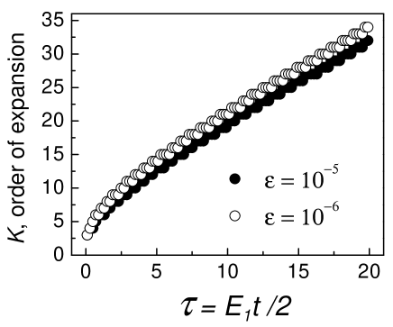
Figure 1: Dependence of the order of the Chebyshev’s expansion $K$ on the value of $\tau=E_{1}t/2$. The solid circles corresponds to the minimum value $\epsilon=10^{-5}$ of the expansion coefficient $c_{k}$; the open circles corresponds to $\epsilon=10^{-6}$.

The high precision of this scheme originates from the fact that, for $k\gg\tau$, the value of a Bessel function decreases super-exponentially $J_{k}(\tau)\sim(\tau/k)^{k}$, so that termination of the series (8) at $k=K$ leads to an error which decreases super-exponentially with $K$. In practice, $K=1.5\tau$ already gives precision of 10^-7 or better in most cases. Due to the same reason, this scheme is asymptotically more efficient than any time-marching scheme. For given sufficiently small error $\epsilon$, the number of operations $Nop$ needed for finding the wavefunction at time $T$, i.e. $\Psi(T)$, grows linearly with $T$ for the Chebyshev-based scheme. For a marching scheme of order $r$ with the time step $\Delta t$, the numerical error is $\epsilon\sim(\Delta t)^{r}T$, so that for given $\epsilon$ and $T$, the number of operations needed is $Nop=T/\Delta t\sim T^{1+1/r}$, growing super-linearly with increasing $T$. For very long-time simulations, and when very high precision is necessary, the Chebyshev method is more efficient than any time-marching scheme known to us. However, in practice, a precision better than 0.5%–1% is very rarely needed. Similarly, very long-time simulations are rarely of interest: in most cases, the simulations are interesting only until the dynamics of the system exhibits some non-trivial behavior. Therefore, in spite of its asymptotic efficiency, the Chebyshev method is not always the best choice for real research, and its efficiency should be studied in every separate case.

IV Simulation results

We assess the usefulness of the Chebyshev’s method for a wide spectrum of decoherence problems, by consideriong two central problems of decoherence, description of damping of quantum oscillations in a system, and determination of the pointer states. In fact, there is no strict boundary: studying both problems, we track evolution of the system checking its state at regular intervals of length $T$, but in studying the oscillations decay the interval $T$ is much smaller than the characteristic decoherence time $T_{dec}$, while in studying the pointer states, $T$ is larger than $T_{dec}$.

In spite of the asymptotic advantages of the Chebyshev-based scheme, it is not a priori clear if it is efficient for realistic problems, when the required numerical error $\delta$ is modest (say, $\delta=10^{-2}$–$10^{-3}$). Also, if we track the dynamics of the decoherence process, we make many steps of modest length $T$, and the overhead associated with the use of the Chebyshev’s expansion might be significant, see Fig. 1.

To study this issue, we have performed several types of numerical tests. The timing information reported in this paper has been obtained from calculations on a SGI Origin 3800 (500 MHz) system, using sequential, single processor code. The order of Chebyshev’s expansion $K$ have been defined by the pre-specified precision $\epsilon$. We determined the minimum value of $K$ such that $|c_{k}|<\epsilon$ for $k\geq K$, starting from the value $K_{0}=[1.1\tau]$ ($[x]$ is the integer part of $x$), and adjusting it as needed. Each simulation has been performed three times: (i) using the Chebyshev’s method with $\epsilon=10^{-12}$, the reference run, (ii) using Chebyshev’s method with $\epsilon=10^{-5}$–10^-6, and (iii) using the scheme based on Suzuki-Trotter decomposition hdr ; hdr1 . Previously we have used the latter to study spin-bath decoherence kondo ; osc . In this paper, we have chosen to consider the same problems as in our previous works on this subject, in order to avoid the impression that the tests have been constructed to favor one particular method.

First, we consider the problem of oscillations damping in the central system of two spins coupled by Heisenberg exchange, interacting with the bath. We studied this problem using the Suzuki-Trotter scheme in Ref. osc, . The Hamiltonians describing the bath and the system are:

$${\cal H}_{S}=J{\bf S}_{1}{\bf S}_{2},\quad{\cal H}_{B}=0,\quad{\cal V}=\sum A_{n}({\bf S}_{1}+{\bf S}_{2}){\bf I}_{n},$$ (11)

with $N=16$ bath spins. The exchange parameter $J=16.0$ (antiferromagnetic coupling between the central spins), while $A_{n}$ are uniformly distributed between 0 and $-0.5$. The initial state of the compound system $|\Psi_{0}\rangle=|\psi_{0}\rangle\otimes|\chi_{0}\rangle$ is the product of the initial state $|\psi_{0}\rangle$ of the central system, and $|\chi_{0}\rangle$ of the bath. In this case, $|\psi_{0}\rangle=|\uparrow\downarrow\rangle$, i.e. the first central spin is in the state $S^{z}_{1}(t=0)=+1/2$, and the second spin is in the state $S^{z}_{2}(t=0)=-1/2$. The initial state of the bath $|\chi_{0}\rangle$ is the linear superposition of all basis states with random coefficients. Physically, this situation corresponds to the case of the temperature $\theta$ which is high in comparison with the bath energies $A_{n}$, but is much lower than the system’s energy $J$ (note that $J\gg A_{n}$ in this case).

Figure 2: Time dependence of the oscillations of the expectation value of $S_{1}^{z}(t)$ in the two-spin system decohered by a spin bath.

The initial state of the central system is a superposition of two eigenstates of ${\cal H}$: the state with the total spin $S=1$ and $S_{z}=0$, and the state with the total spin $S=0$. These states have different energies, and, for example, the dynamics of $S^{z}_{1}(t)$ is represented by oscillations with the frequency $J$. Due to interaction with the spin bath, these oscillations are damped, see Fig. 2. To study this damping in detail, we take the Suzuki-Trotter time step $\Delta t=0.035$, $T=2\Delta t$, and watch the system since $t=0$ till $t_{max}=800T$. If we do not need such a high resolution, we increase $T$. In Table 1, we present the CPU time needed to perform the simulations using the Suzuki-Trotter and Chebyshev’s methods, along with the resulting error $\delta$ (which should not be confused with the “nominal” precision of the Chebyshev’s scheme $\epsilon$). The error $\delta$ has been obtained from comparison with the “reference” Chebyshev’s run ($\epsilon=10^{-12}$), and is equal to the maximum of absolute errors of the quantities (all normalized to unity) $2S^{\alpha}_{1}$, $2S^{\alpha}_{2}$, $4S^{\alpha}_{1}S^{\beta}_{1}$ ($\alpha,\beta=x,y,z$), and the so-called “quadratic entropy” quent $S^{(2)}=1-\mathop{\rm Tr}\rho^{2}_{S}$. These quantities have been calculated and compared at regular intervals of length $T$. Their calculation increases the number of computations, so that the tests 1, 2, and 3, which are otherwise equivalent for the Suzuki-Trotter method, require more and more CPU time.

Table 1: Comparison of the Suzuki-Trotter scheme (abbreviated as ST) with the Chebyshev’s scheme (abbreviated as Ch) for the problem of oscillations decay.

Test	$\Delta t$	$T$	$t_{max}$	$\delta$	$\epsilon$	CPU Time
1, Ch	—	$200\Delta t$	$8T$	$1\cdot 10^{-5}$	$10^{-6}$	22 min
1, ST	0.035	$200\Delta t$	$8T$	$0.44\cdot 10^{-2}$	—	80 min
2, Ch	—	$8\Delta t$	$200T$	$0.3\cdot 10^{-4}$	$10^{-6}$	59 min
2, ST	0.035	$8\Delta t$	$200T$	$0.48\cdot 10^{-2}$	—	89 min
3, Ch	—	$2\Delta t$	$800T$	$0.55\cdot 10^{-3}$	$10^{-6}$	226 min
3, ST	0.035	$2\Delta t$	$800T$	$0.48\cdot 10^{-2}$	—	156 min

As one can see from Table 1, for realistic values of maximum error $\delta\sim 0.5\cdot 10^{-2}$, and even for not very long runs, the Chebyshev’s scheme can be faster than the Suzuki-Trotter method by a factor of up to four, and the efficiency of the Chebyshev’s scheme grows fast with increasing $T$. However, this straightforward comparison is too crude, and Table 1 is only an illustration of basic features of the Chebyshev’s method. To model fast oscillations which decay slowly (often, with the decay time of order of decoherence time $T_{dec}$), we should make $T$ significantly smaller than the oscillation period $t_{osc}=2\pi/J$, in order to correctly determine the amplitude of oscillations at given time.

Therefore, to track the damping of oscillations, we use the two-leap approach: first, we make a large time leap of length $T_{1}$ ($T_{1}\gg t_{osc}$, but $T_{1}\ll T_{dec}$), and then we make a number $n_{2}$ (usually, 15–20) of smaller steps $T_{2}$ such that $T_{2}\ll t_{osc}$ but $n_{2}T_{2}\geq t_{osc}$, resolving in detail one period of oscillations and extracting the amplitude. By repeating this two-stage sequence $n_{tot}$ times, we can reliably track the change of the oscillations amplitude with time. The test example of this approach have been taken from our recent work akakii . We have performed the same kind of simulations as described above, with $N=16$ bath spins, repeating the two-leap sequence $n_{tot}=8$ times, each time making one long leap $T_{1}$ followed by $n_{2}=21$ short leaps $T_{2}$. The results of these tests are presented in Table 2. Again, Chebyshev-based method can be up to three times faster than the Suzuki-Trotter algorithm hdr ; hdr1 .

Table 2: Comparison of the Suzuki-Trotter scheme (abbreviated as ST) with the Chebyshev’s scheme (abbreviated as Ch) for the problem of oscillations decay, employing the two-leap approach with different $T_{1}$ and $T_{2}$.

Test	$\Delta t$	$T_{1}$	$T_{2}$	$\delta$	$\epsilon$	CPU Time
4, Ch	—	$150\Delta t$	$\Delta t$	$0.4\cdot 10^{-4}$	$10^{-6}$	61 min
4, ST	0.02	$150\Delta t$	$\Delta t$	$0.2\cdot 10^{-2}$	—	144 min
5, Ch	—	$300\Delta t$	$\Delta t$	$0.4\cdot 10^{-4}$	$10^{-6}$	75 min
5, ST	0.02	$300\Delta t$	$\Delta t$	$0.3\cdot 10^{-2}$	—	221 min

Finally, we have tested the Chebyshev scheme in the problem of determining the pointer states, employing an example from our work kondo . This example is interesting also because it deals with a physically important case of a spin bath possessing chaotic internal dynamics, which is relevant for majority of realistic spin baths (such as nuclear spins or impurity spins baths). The Hamiltonian describing the system is

$${\cal H}_{S}=J{\bf S}_{1}{\bf S}_{2},\quad{\cal V}=\sum A_{n}{\bf S}_{1}{\bf I}_{n},$$ (12)

i.e., the bath spins are coupled only with the first central spin, and the bath Hamiltonian is now

$${\cal H}_{B}=\sum_{n}h_{z}I^{z}_{k}+\sum_{\langle n,n^{\prime}\rangle}U_{nn^{\prime}}I^{x}_{n}I^{x}_{n^{\prime}}.$$ (13)

In our simulations we used $h=0.1$ and $U_{nn^{\prime}}$ randomly distributed in the interval $[-0.013,0.013]$. This Hamiltonian is known to result in stochastic behavior shepel ; we have checked the level statistics independently, and found that it closely follows the Wigner-Dyson distribution.

To determine the pointer states, we need to find the elements of the reduced density matrix $\rho_{S}(t)$ in the long-time limit $t\to\infty$. We start at $t=0$ from the state of the compound system which is the product of the states of the bath and the central system (as above), but the initial state of the central spins now is the singlet $|\psi_{0}\rangle=(1/\sqrt{2})[|\uparrow\downarrow\rangle-|\downarrow\uparrow\rangle]$. Because of decoherence, the final state of the central system is mixed, and $\rho_{S}=w_{1}|p_{1}\rangle\langle p_{1}|+w_{2}|p_{2}\rangle\langle p_{2}|$, where $|p_{1}\rangle$ and $|p_{2}\rangle$ are the pointer states, which are superpositions of the states $|\uparrow\uparrow\rangle$, $|\downarrow\downarrow\rangle$ $|\uparrow\downarrow\rangle$, and $|\downarrow\uparrow\rangle$. As we have found in our work kondo , the form of this superposition is determined by the ratio $J/b$, where $b=\sum_{n}A^{2}_{n}$. For $J/b\sim 1$, the pointer states are very close to the singlet $S=0$ and triplet $S=1$, $S_{z}=0$ states, and for $J\ll b$, the pointer states are close to $|\uparrow\downarrow\rangle$ and $|\downarrow\uparrow\rangle$. Thus, the quantities characterizing the type of the pointer state are the values of the non-diagonal elements of the density matrix $\rho_{S}$ in the basis $|\uparrow\uparrow\rangle$, $|\downarrow\downarrow\rangle$ $|\uparrow\downarrow\rangle$, and $|\downarrow\uparrow\rangle$. In particular, the element $\rho^{12}_{S}=\langle\uparrow\downarrow|\rho_{S}|\downarrow\uparrow\rangle$ is a very suitable quantity to characterize the pointer state. This non-diagonal element is close to zero for $J\ll b$, and gradually increases in absolute value with increasing $J$.

Figure 3: Temporal evolution of different elements of the density matrix $\rho$: diagonal elements corresponding to the states $|\uparrow\uparrow\rangle$, $|\uparrow\downarrow\rangle$, $|\downarrow\uparrow\rangle$, and $|\downarrow\downarrow\rangle$ (the four upper curves), and the non-diagonal element $\rho^{12}_{S}$ (the lowest curve). Very slow relaxation is better seen for the uppermost curve (the diagonal element corresponding to the state $|\uparrow\uparrow\rangle$) which has a small negative slope. Note that the two lines in the middle (the second and the third lines from above, the diagonal elements corresponding to the states $|\uparrow\downarrow\rangle$ and $|\downarrow\uparrow\rangle$, correspondingly) are very close to each other at $t\geq 200$, as expected for a near-equilibrium (although not completely relaxed) situation.

Typical results for temporal evolution of the elements of the density matrix $\rho_{S}$ are shown in Fig. 3. One can see that in this situation, we do not need to use the two-leap approach with different $T_{1}$ and $T_{2}$. The relaxation (after some initial period) is slow, and no fast oscillations of considerable amplitude exist at long times, so that the one-leap approach is sufficient. Thus, the efficiency of the Chebyshev-based scheme is expected to be very good. This is indeed the case, as Table 3 demonstrates. The results presented there correspond to $J=0.1$. The Chebyshev-based scheme is faster than the Suzuki-Trotter method up to a factor of 8.

Table 3: Comparison of the Suzuki-Trotter scheme (abbreviated as ST) with the Chebyshev’s scheme (abbreviated as Ch) for the problem of determining the pointer states.

Test	$\Delta t$	$T$	$t_{max}$	$\delta$	$\epsilon$	CPU Time
6, Ch	—	$100\Delta t$	$500T$	$0.2\cdot 10^{-3}$	$10^{-6}$	19 min
6, ST	0.14	$100\Delta t$	$500T$	$0.7\cdot 10^{-2}$	—	105 min
7, Ch	—	$10\Delta t$	$5000T$	$0.1\cdot 10^{-2}$	$10^{-6}$	52 min
7, ST	0.14	$10\Delta t$	$5000T$	$0.8\cdot 10^{-2}$	—	117 min
8, Ch	—	$1000\Delta t$	$50T$	$0.3\cdot 10^{-6}$	$10^{-6}$	13 min
8, ST	0.14	$1000\Delta t$	$50T$	$0.8\cdot 10^{-2}$	—	107 min

We have checked our conclusions on many other cases, with the central systems made of up to $M=4$ spins, and with the baths made of up to $N=22$ spins, with different Hamiltonians and different values of the Hamiltonian parameters. We found that Chebyshev-based method gives a significant increase in the simulations speed for all problems where the value of $T$ can be made sufficiently large.

V Summary

Theoretical studies of the spin-bath decoherence are important for many areas of physics, including quantum mechanics and quantum measurement theory, quantum computing, solid state physics etc. Decoherence is a complex many-body phenomenon, and numerical simulation is an important tool for its investigation. In this paper, we have studied efficiency of the numerical scheme based on the Chebyshev expansion. We have presented specific details of the application of this method to the spin-bath decoherence modeling. To assess the efficiency of the simulation method, we have used model problems which we have encountered in our previous studies of the spin-bath decoherence. We compared the Chebyshev-based scheme with a fast method based on the Suzuki-Trotter decomposition. We have found that in many cases, the former gives a considerable increase in the speed of simulations, sometimes up to a factor of eight (for the problem of finding the system’s pointer states), while in studying the decoherence dynamics, the increase in speed is less drastic (a factor of 2–3), but still considerable. This conclusion holds for many types of central systems and spin baths, with different Hamiltonians.

- (1) M. A. Nielsen, I. L. Chuang, Quantum computation and quantum information (Cambridge University Press, Cambridge, New York, 2000).
- (2) D. P. DiVincenzo, “The physical implementation of quantum computation”, quant-ph/0002077.
- (3) J. Preskill, Proc. R. Soc. London, Ser. A 454, 385 (1998).
- (4) Decoherence: Theoretical, Experimental and Conceptual Problems, eds. Ph. Blanchard, D. Giulini, E. Joos, C. Kiefer, I.-O. Stamatescu, (Springer-Verlag, Berlin, Heidelberg, New York,2000)
- (5) D. Giulini, E. Joos, C. Kiefer, J. Kupsch, I.-O. Stamatescu, H. D. Zeh, Decoherence and the Appearance of a Classical World in Quantum Theory (Springer-Verlag, Berlin, Heidelberg, New York, 1996).
- (6) W. H. Zurek, Phys. Rev. D 24, 1516 (1981), Phys. Rev. D 26, 1862 (1982); E. Joos and H. D. Zeh, Z. Phys. B 59, 223 (1985).
- (7) A. J. Leggett, S. Chakravarty, A. T. Dorsey, M. P. A. Fisher, A. Garg, and W. Zwerger, Rev. Mod. Phys. 59, 1 (1987).
- (8) Quantum Tunneling of Magnetization — QTM’94, eds. L. Gunther and B. Barbara, NATO ASI Ser. E, Vol. 301 (Kluwer, Dordrecht, 1995)
- (9) K. Saito, S. Miyashita, and H. De Raedt, Phys. Rev. B 60, 14553 (1999)
- (10) M. I. Katsnelson, V. V. Dobrovitski, H. A. De Raedt, and B. N. Harmon, “Destruction of the Kondo effect by a local measurement”, cond-mat/0205540.
- (11) K. Saito, S. Takesue, and S. Miyashita, J. Phys. Soc. Jpn. 65, 1243 (1996)
- (12) H. Tal-Ezer, SIAM J. Numer. Anal. 23, 11 (1986); ibid. SIAM J. Numer. Anal. 26, 1 (1989).
- (13) H. Tal-Ezer and R. Kosloff, J. Chem. Phys. 81, 3967 (1984).
- (14) C. Leforestier, R.H. Bisseling, C. Cerjan, M.D. Feit, R. Friesner, A. Guldberg, A. Hammerich, G. Jolicard, W. Karrlein, H.-D. Meyer, N. Lipkin, O. Roncero, and R. Kosloff, J. Comp. Phys. 94, 59 (1991).
- (15) R. Kosloff, Ann. Rev. Phys. Chem. 45, 145 (1994).
- (16) T. Iitaka, S. Nomura, H. Hirayama, X. Zhao, Y. Aoyagi, and T. Sugano, Phys. Rev. E 56, 1222 (1997).
- (17) R.N. Silver and H. Röder, Phys. Rev. E 56, 4822 (1997).
- (18) Y.L. Loh, S.N. Taraskin, and S.R. Elliott, Phys. Rev. Lett. 84, 2290 (2000); ibid. 84, 5028 (2000).
- (19) P. de Vries and H. De Raedt, Phys. Rev. B47, 7929 (1993)
- (20) H. De Raedt, A.H. Hams, K. Michielsen, and K. De Raedt, Comp. Phys. Comm. 132, 1 (2000)
- (21) M. Suzuki, S. Miyashita, and A. Kuroda, Prog. Theor. Phys. 58, 1377 (1977)
- (22) U. Manthe, H. Köppel, and L. S. Cederbaum, J. Chem. Phys. 95, 1708 (1991).
- (23) J. Jaklič, and P. Prelovšek, Adv. Phys. 49, 1 (2000).
- (24) M. H. Beck, A. Jäckle, G. A. Worth, and H.-D. Meyer, Phys. Rep. 324, 1 (2000).
- (25) H. Wang, J. Chem. Phys. 113, 9948 (2000).
- (26) M. Thoss, H. Wang, and W. H. Miller, J. Chem. Phys. 115, 2991 (2001).
- (27) V. V. Dobrovitski, H. A. De Raedt, M. I. Katsnelson, and B. N. Harmon, “Quantum oscillations without quantum coherence”, quant-ph/0112053.
- (28) Quadratic entropy characterizes, how mixed is the state of the central system; for pure states .
- (29) A. Melikidze, V. V. Dobrovitski, H. A. De Raedt, M. I. Katsnelson, and B. N. Harmon, “Parity effects in spin decoherence”, (to be published); quant-ph/0212097.
- (30) B. Georgeot and D. L. Shepelyansky, Phys. Rev. E 62, 6366 (2000).