Decoherence and Quantum-state Measurement in Quantum Optics
11institutetext: Instituto de Física, Universidade Federal do Rio de Janeiro
Rio de Janeiro, RJ 21941-972, BRAZIL
Decoherence and Quantum-state Measurement in Quantum Optics
Abstract
This paper discusses work developed in recent years, in the domain of quantum optics, which has led to a better understanding of the classical limit of quantum mechanics. New techniques have been proposed, and experimentally demonstrated, for characterizing and monitoring in real time the quantum state of an electromagnetic field in a cavity. They allow the investigation of the dynamics of the decoherence process by which a quantum-mechanical superposition of coherent states of the field becomes a statistical mixture.
1 Introduction
One of the most subtle problems in contemporary physics is the relation between the macroscopic world, described by classical physics, and the microscopic world, ruled by the laws of quantum mechanics. Among the several questions involved in the quantum-classical transition, one stands out in a striking way. As pointed out by Einstein in a letter to Max Born in 1954 Einstein , it concerns “the inexistence at the classical level of the majority of states allowed by quantum mechanics,” namely coherent superpositions of classically distinct states. Indeed, while in the quantum world one frequently comes across coherent superpositions of states (like in Young’s two-slit interference experiment, in which each photon is considered to be in a coherent superposition of two wave packets, centered around the classical paths which stem out of each slit), one does not see macroscopic objects in coherent superpositions of two distinct classical states, like a stone which could be at two places at the same time. There is an important difference between a state of this kind and one which would involve just a classical alternative: the existence of quantum coherence between the two localized states would allow in principle the realization of an interference experiment, complementary to the simple observation of the position of the object. We know all this already from Young’s experiment: the observation of the photon path (that is, a measurement able to distinguish through which slit the photon has passed) unavoidably destroys the interference fringes.
If one assumes that the usual rules of quantum dynamics are valid up to the macroscopic level, then the existence of quantum interference at the microscopic level necessarily implies that the same phenomenon should occur between distinguishable macroscopic states. This was emphasized by Schrödinger in his famous “cat paradox” Schrodinger . An important role is played by this fact in quantum measurement theory, as pointed out by Von Neumann Von Neumann . Indeed, let us assume for instance that a microscopic two-level system (states and ) interacts with a macroscopic measuring apparatus, in such a way that the pointer of the apparatus points to a different (and classically distinguishable!) position for each of the two states, that is, the interaction transforms the joint atom-apparatus initial state into
where one has allowed for a change in the state of the two-level system, due to its interaction with the measurement apparatus.
The linearity of quantum mechanics implies that, if the quantum system is prepared in a coherent superposition of the two states, say , the final state of the complete system should be a coherent superposition of two product states, each of which corresponding to a different position of the pointer:
where in the last step it was assumed that the two-level system is incorporated into the measurement apparatus after their interaction (for instance, an atom that gets stuck to the detector). One gets, therefore, as a result of the interaction between the microscopic and the macroscopic system, a coherent superposition of two classically distinct states of the macroscopic apparatus. This is actually the situation in Schrödinger’s cat paradox: the cat can be viewed as a measuring apparatus of the state of a decaying atom, the state of life or death of the cat being equivalent to the two positions of the pointer. This would imply that one should be able in principle to get interference between the two states of the pointer: it is precisely the lack of evidence of such phenomena in the macroscopic world that motivated Einstein’s concern.
Faced with this problem, Von Neumann introduced through his collapse postulate Von Neumann two distinct types of evolution in quantum mechanics: the deterministic and unitary evolution associated to the Schrödinger equation, which describes the establishment of a correlation between states of the microscopic system being measured and distinguishable classical states (for instance, distinct positions of a pointer) of the macroscopic measurement apparatus; and the probabilistic and irreversible process associated with measurement, which transforms coherent superpositions of distinguishable classical states into statistical mixtures. This separation of the whole process into two steps has been the object of much debate Wigner ; Wheeler ; Hepp ; indeed, it would not only imply an intrinsic limitation of quantum mechanics to deal with classical objects, but it would also pose the problem of drawing the line between the microscopic and the macroscopic world.
Several possibilities have been explored as solutions to this paradox, including the proposal that a small non-linear term in the Schrödinger equation, although unnoticeable for microscopic phenomena, could eliminate the coherence between distinguishable macroscopic states, thus transforming the quantum superpositions into statistical mixtures Wigner . The non-observability of the coherence between the two positions of the pointer has been attributed both to the lack of non-local observables with matrix elements between the two corresponding states Gottfried as well as to the fast decoherence due to interaction with the environment Zurek ; Caldeira ; Haake . This last approach has been emphasized in recent years: decoherence follows from the irreversible coupling of the observed system to a reservoir Zurek ; Caldeira . In this process, the quantum superposition is turned into a statistical mixture, for which all the information on the system can be described in classical terms, so our usual perception of the world is recovered. Furthermore, for macroscopic superpositions quantum coherence decays much faster than the macroscopic observables of the system, its decay time being given by the dissipation time divided by a dimensionless number measuring the “separation” between the two parts. The statement that these two parts are macroscopically separated implies that this separation is an extremely large number. Such is the case for biological systems like “cats” made of huge number of molecules. In the simple case mentioned by Einstein Einstein , of a particle split into two spatially separated wave packets by a distance , the dimensionless measure of the separation is , where is the particle de Broglie wavelength. For a particle with mass equal to 1 g at a temperature of 300 K, and cm, this number is about , and the decoherence is for all purposes instantaneous. This would provide an answer to Einstein’s concern: the decoherence of macroscopic states would be too fast to be observed.
In this paper, it will be shown that the study of the interaction between atoms and electromagnetic fields in cavities can help us understand some aspects of this problem. In fact, many recent contributions in the field of quantum optics have led not only to the investigation of the subtle frontier between the quantum and the classical world, but also of hitherto unsuspected quantum mechanical processes like teleportation. Research on quantum optics is therefore intimately entangled with fundamental problems of quantum mechanics.
The whole area of “cavity quantum electrodynamics” is a very recent one. It concerns the interactions between atoms and discrete modes of the electromagnetic field in a cavity, under conditions such that losses due to dissipation and atomic spontaneous emission are very small. Usually, one deals with atomic beams crossing cavities with a high quality factor (defined as the product of the angular frequency of the mode and its lifetime, ). The atoms, prepared in special states and detected after interacting with the field, serve two purposes: they are used to manipulate the field in the cavity, so as to produce the desired states, and also to measure the field.
Several factors contributed to the development of this area. The production of superconducting Niobium cavities, with extremely high quality factors, up to the order of , allows one to keep a photon in the cavity for a time of the order of a fraction of a second. New techniques of atomic excitation (alkaline atoms, like Rubidium and Cesium, are frequently used for this purpose) to highly excited levels (principal quantum numbers of the order of 50), and with maximum angular momentum () — the so-called planetary Rydberg atoms — have led to the production of atomic beams that interact strongly even with very weak fields, of the order of one photon, due to the large magnitude of the relevant electric dipoles. Besides, the lifetime of these states is large — of the order of the millisecond — which may be understood semiclassically, from the correspondence principle (which should be valid for ): the electron is always very far away from the nucleus, and therefore its acceleration is small, implying weak radiation and a long lifetime. One should also mention the new techniques of atomic velocity control, which allow the production of approximately monokinetic atomic beams, leading to a precise control of the interaction time between atom and field. For a review of some of the main problems and results in this field, see Haroche .
2 Coherent Superpositions of Mesoscopic States in Cavity QED
2.1 Building the Coherent Superposition
We show now how, by carefully tailoring the interactions between two-level atoms and one mode of the electromagnetic field in a cavity, one can produce quantum superpositions of distinguishable coherent states of the field, thus mimicking the superposition of two classically distinct states of a pointer.
For a harmonic oscillator, a coherent state Glauber is obtained by displacing the ground state in phase space. In general, the position will be displaced by and the momentum by , so that the displacement can be characterized by the complex amplitude , where and are respectively the mass and the angular frequency of the oscillator. The state is thus denoted by , and it can be physically realized by applying a classical force to the oscillator. Coherent states are “quasi-classical” states: they evolve in time without changing their shape, the corresponding wave packet oscillating around the equilibrium position like a classical particle. Furthermore, they are minimum-uncertainty states: the product of the uncertainties in position and momentum is equal to the minimum value allowed by the Heisenberg uncertainty principle.
A one-mode electromagnetic field can be described by a harmonic oscillator Hamiltonian, in which the position and momentum are replaced by the quadratures of the field. These are defined as the amplitudes and of the cosine and sine terms in the time-dependent expression of the field:
| (1) |
This expression is analogous to the one that yields the position of a harmonic oscillator at time , as a function of the initial position and momentum:
| (2) |
so that the quadratures and play a role analogous to the position and momentum (conveniently normalized). In the same way that, in quantum mechanics, the position and momentum are non-commuting operators, quantization of the electromagnetic field is achieved by requiring that the operators corresponding to the quadratures, and , satisfy . They are related to the photon annihilation operator by
| (3) |
The complex amplitude of the field is defined as .
For an electromagnetic field, a coherent state also corresponds to a displaced ground state (in this case the vacuum state of the electromagnetic field). It can be explicitly written as (for a one-mode field)
| (4) |
where is the vacuum state of the electromagnetic field and is the displacement operator. The average number of photons in the coherent state is Glauber . This state can be physically realized by turning on a classical current (for instance, a microwave generator) when the field is in the vacuum state. The corresponding evolution operator in the interaction picture is then closely related to the displacement operator.
The method for generating the quantum superposition of two coherent states, proposed in Brune , and sketched in Fig. 1, involves a beam of circular Rydberg atoms Kleppner crossing a high- cavity C in which a coherent state is previously injected (this is accomplished by coupling the cavity to a classical source – a microwave generator – through a wave guide). The utilization of circular levels is due to their strong coupling to microwaves and their very long radiative decay times, which makes them ideally suited for preparing and detecting long-lived correlations between atom and field states Brune2 . On either side of the high- cavity there are two low- cavities ( and ), which remain coupled to a microwave generator. The fields in these two cavities can be considered as classical. As a matter of fact, it can be shown that, for the experiments realized so far, the average number of photons in these cavities is of the order of one. How come then this field behaves classically? This is due to the highly dissipative character of these cavities: again, dissipation helps to turn the quantum-mechanical world into a classical one. The classical behavior of the fields in these low- cavities was demonstrated in Ji .
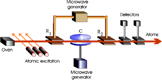
This set of two low-Q cavities constitutes the usual experimental arrangement in the Ramsey method of interferometry Brune2 ; Ramsey . Two of the (highly excited) atomic levels, which we denote by (the upper level) and (the lower one), are resonant with the microwave fields in cavities and . The interaction of a two-level atom with a resonant electromagnetic field is analogous to the interaction between a spin and a magnetic field: it amounts to a rotation transformation applied to the two states. The intensity of the fields in and is chosen so that, for the selected atomic velocity, effectively a pulse is applied to the atom as it crosses each cavity. For a properly chosen phase of the microwave field, this pulse transforms the state into the linear combination , and the state into .
Therefore, if each atom is prepared in the state just prior to crossing the system, after leaving the atom is in a superposition of two circular Rydberg states and :
| (5) |
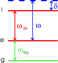
On the other hand, the superconducting cavity is assumed not to be in resonance with any of the transitions originating from those two atomic states. This means that the atom does not suffer a transition, and does not emit or absorb photons from the field. This property is further enhanced by the fact that the cavity mode is such that the field slowly rises and decreases along the atomic trajectory, so that, for sufficiently slow atoms, the atom-field coupling is adiabatic. However, the cavity is tuned in such a way that it is much closer to resonance with respect to one of those transitions, say the one connecting to some intermediate state . The relevant level scheme is illustrated in Fig. 2. This implies that, if the atom crosses the cavity in state , dispersive effects can induce an appreciable phase shift on the field in the cavity. That is, the atom acts like a refraction index, changing the frequency of the field while the interaction is on — the corresponding energy change is just the AC-Stark shift, which for a Fock state of the electromagnetic field is proportional to the number of photons in the cavity. This frequency shift, multiplied by the interaction time between the atom and the mode, leads to a phase shift of the field in the cavity, if the atom is in state . The phase shift is negligible, however, if the atom is in state . For a principal quantum number equal to 50 in the state , and the cavity tuned close to the circular to circular transition (around 50 GHz), a phase shift of the order of per photon is produced by an atom crossing the centimeter size cavity with a velocity of about 100 m/s Brune .
Note that, if there is a coherent state in the cavity, a phase shift of per photon if the atom is in state implies that
| (6) |
that is, the phase of the coherent state is shifted by . The above equation makes use of the expansion of a coherent state in terms of Fock states.
After the atom has crossed the cavity, in a time short compared to the field relaxation time and also to the atomic radiative damping time, the state of the combined atom-field system can be written as
| (7) |
assuming that the phase shift is per photon if the atom is in the excited state. The entanglement between the field and atomic states is analogous to the correlated two-particle states in the Einstein-Podolski-Rosen (EPR) paradox.EPR ; Bell ; Aspect The two possible atomic states and are here correlated to the two field states and , respectively. After the atoms leave the superconducting cavity, one can detect them in the or states, by sending them through two ionization chambers, the first one having a field smaller than the second, so that it ionizes the atom in the state, but not in the state, while the second ionizes the atoms that remain in state (Fig. 1). In the actual experiment, this detection system is replaced by a single chamber, with a static electric field that increases linearly along the direction of atomic motion. This measurement projects the field in the cavity either onto the state (if the atom is detected in state ), or onto the state (if the atom is detected in state ). However, as in an EPR experiment Aspect , one may choose to make another kind of measurement, letting the atom cross, after it leaves the superconducting cavity, a second classical microwave field ( in Fig. 1), which amounts to applying to the atom another pulse. The state (7) gets transformed then into
| (8) |
If one detects now the atom in the state or , the field is projected onto the state
| (9) |
where and or , according to whether the detected state is or , respectively. One produces therefore a coherent superposition of two coherent states, with phases differing by . For , this is a “Schrödinger cat-like” state.
2.2 Measuring the Coherent Superposition
Once the quantum superposition is produced, how could one tell the difference between such a superposition and a statistical mixture of the two coherent states? This can be done by simply sending another atom, in the same initial state as the first one. It can be shown then Luiz2 that, for the state (9), with , there is a perfect correlation between the measurements of the first and the second atom: both are always detected in the same state. On the other hand, for the corresponding statistical mixture the probability of detecting the second atom in state is 50%, independently of which state was detected for the first atom. By delaying the sending of the second atom, one may thus explore the dynamical process by which the quantum superposition is transformed into a statistical mixture, due to the always present dissipation in a non-perfect cavity.
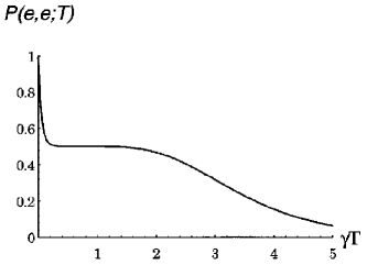
The time-dependent behavior of the conditional probability for measuring the second atom in the upper state, knowing that the first atom was also measured in the upper state, is displayed in Fig. 3. The sharp decay of this conditional probability from the perfectly coherent situation to the plateau associated with an incoherent superposition defines the decoherence time. This time can be shown to be equal to the dissipation time for the field in the cavity divided by twice the average number of photons in the field. Thus, it becomes shorter as the field becomes more macroscopic. Note also that the plateau eventually disappears, and the probability for measuring the second atom in the state goes to zero. This can be easily understood: the field in the cavity C leaks out, and therefore the sole effect on the atom initially prepared in the state is the sum of two pulses in the cavities and , that is a pulse, which takes the atom into the state .
An experimental realization of this proposal was made in 1996 by Haroche’s group at Ecole Normale Supérieure, in Paris Brune3 . The dynamical measurement of the decoherence process, as proposed above, was in agreement with the theoretical predictions.
3 The Wigner Distribution
One might wonder if it could be possible to get, from the above experimental setup, a more complete information on the field in the cavity. This was shown to be indeed possible in Lutter : a slight modification of the above experiment leads to the reconstruction of the so-called Wigner distribution of the field in the cavity, which provides a complete description of the quantum state of the field in phase space.
Phase space probability distributions are very useful in classical statistical physics. Averages of relevant functions of the positions and momenta of the particles can be obtained by integrating these functions with those probability weights.
In quantum mechanics, similar averages are calculated by taking the trace of the product of the density operator that describes the system with the observable of interest. Heisenberg’s inequality forbids the existence in phase space of bonafied probability distributions, since one cannot determine simultaneously the position and the momentum of a particle. In spite of this, phase space distributions may still play a useful role in quantum mechanics, allowing the calculation of the average of operator-valued functions of the position and momentum operators as classical-like integrals of -number functions. These functions are associated to those operators through correspondence rules, which depend on a previously defined operator ordering.
From all phase space representations, the Wigner distribution Wigner2 is the most natural one, when one looks for a quantum-mechanical analog of a classical probability distribution in phase space. It is in fact the only distribution that leads to the correct marginal distributions, for any direction of integration in phase space Bertrand ; Ulf . Let us consider for simplicity a one-dimensional problem, for a particle with position and momentum . We take these to be dimensionless variables, measured in terms of some typical position and momentum of the system, which play the role of natural units (for a harmonic oscillator, the natural units would be the uncertainties in position and momentum of the ground state). If the state of the particle is characterized by the density operator , then we should have not only
| (10) |
where and are eigenstates of the operators and , respectively, but also
| (11) |
where now
| (12) |
the rotated coordinate being defined as
| (13) |
One should note that, for a pure state, . One should also note that from (10) it follows immediately the normalization property:
| (14) |
Expression (11), which yields the probability distribution for in terms of the function , is called a Radon transform. Note that this transform may be defined independently of quantum mechanics, and in fact it was investigated in 1917 by the mathematician Johan Radon Radon . He showed that, if one knows for all angles , then one can uniquely recover the function , through the so-called Radon inverse transform. Quantum mechanics comes into play if one now identifies , given by the Radon transform (11), with the quantum expression (12). It follows then that (11) and (12) uniquely determine the function , in terms of the density operator of the system. The function is in this case precisely the Wigner function of the system, expressed in terms of the density matrix in the position representation by
| (15) |
which, except for a normalization constant, is the famous expression written down by Wigner Wigner2 in his article “On the Quantum Correction for Thermodynamic Equilibrium,” published in 1932.
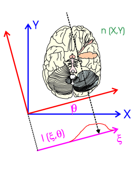
The demonstration of this result can be found in Bertrand ; Ulf . Let us note that Radon’s result is the mathematical basis of tomography. In fact, application of this procedure to medicine (see Fig. 4) has brought the Nobel prize in Medicine to Cormack and Hounsfield in 1979.
The tomographic procedure has a simple interpretation for a harmonic oscillator. From (2), it is clear that in this case measuring the quadratures for all angles is equivalent to measuring the position of the harmonic oscillator for all times from to . This implies that the measurement of for allows one to reconstruct the state of the harmonic oscillator.
The question about what is the minimum set of measurements needed to reconstruct the state of a system is actually a very old problem in quantum mechanics. In his article on quantum mechanics in the Handbuch der Physik in 1933 Pauli , Pauli stated that “the mathematical problem, as to whether for given functions and [probability distributions in position and momentum space], the wave function , if such a function exists, is always uniquely determined has still not been investigated in all its generality.” One knows now the answer to this question: the probability distributions and do not form a complete set in the tomographic sense, and therefore are not sufficient to determine uniquely the quantum state of the system.
In 1949, it was shown by Moyal Moyal that the Wigner distribution can be used to calculate averages of symmetric operator functions of and , as classical-like integrals in phase space. Thus, for instance,
| (16) |
where is the Wigner function corresponding to the density operator .
For a harmonic oscillator, an alternative expression for the Wigner function may be obtained by expressing the position and momentum operators and (or, alternatively, the quadrature operators and ) in terms of the annihilation and creation operators and , defined by (3).
One gets then Cahill :
| (17) |
where the displacement operator is defined by (4). Since is the parity operator (note that , ), this expression shows that the Wigner function is proportional to the average of the displaced parity operator.
The Wigner function given by (17) involves actually a different normalization with respect to the one defined by (15): one must set , so that
| (18) |
It is easy to check that the Wigner function is real and bounded. With the normalization (18), it satisfies the bound
| (19) |
However, it may become negative: this is related to the fact that a bonafied phase space distribution cannot exist in quantum mechanics.
3.1 Measuring the Wigner Function
It was only in 1989 that Risken and Vogel suggested that the technique of homodyne detection could be used to reconstruct the Wigner function of a running electromagnetic wave Vogel . Indeed, this technique allows the measurement of the probability distribution of an arbitrary quadrature of the electromagnetic field , and one is then able to reconstruct the Wigner function through the inverse Radon transform.
The first experimental demonstration of this procedure was achieved in 1993 by Smithey et al Smithey . In view of the low detection efficiency in those experiments, the detected distribution was actually a smoothed version of the Wigner function, closely related to the so-called Husimi distribution. A much better result was achieved by Mlynek’s group in 1995 Mlynek , clearly displaying a highly compressed Gaussian, corresponding to the experimentally obtained Wigner function of a squeezed state of light emerging from an optical parametric oscillator (squeezed states are minimum uncertainty states such that the variance of one of the quadratures is smaller than the one corresponding to the vacuum state of the field). A procedure closely related to the homodyne detection method was used to reconstruct the vibrational state of a molecule by T. J. Dunn et al Dunn .
Using a different (but also indirect) method, the Wigner function of the center-of-mass state of an ion trapped in a harmonic trap, and placed in the first excited state of the harmonic potential, was measured by Wineland’s group at NIST Leibfried .
3.2 Examples of Wigner Functions
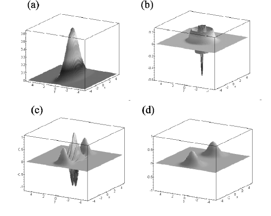
Some examples of Wigner functions are shown in Fig. 5. The Wigner function corresponding to the ground state of a harmonic oscillator (or the vacuum of the electromagnetic field) is a Gaussian, centered around the origin of phase space. For a squeezed state, one gets a compressed Gaussian. On the other hand, for eigenstates of the harmonic oscillator – corresponding, for an electromagnetic field, to states with well-defined number of photons – the Wigner function is negative in some regions of phase space, as shown in Fig. 5(b). As mentioned before, this is an evidence that it cannot be considered a bonafied probability distribution. Note also that, while the statistical mixture of two coherent states (which are displaced ground states) corresponds to a sum of two Gaussians, the Wigner function corresponding to the quantum superposition of two coherent states exhibits interference fringes, a clear signature of coherence. Decoherence leads to the disappearance of these fringes. Therefore, the measurement of the Wigner function of the electromagnetic field would be a clear-cut way of distinguishing between a coherent superposition and a mixture of the two coherent states. Furthermore, if one could make this measurement fast enough, one would be able to follow the decoherence process in real time.
4 Direct Measurement of the Wigner Function
Once the proper state of the field is produced in the cavity, how would one be able to measure it? As shown in Lutter ; Lutter2 , it is actually possible to measure the Wigner function of the field by a relatively simple scheme, which provides directly the value of the Wigner function at any point of phase space. This is in contrast with the tomographic procedure, or the method adopted at NIST, which yield the Wigner function only after some integration or summation. Furthermore, and also in contrast with those methods, the scheme proposed in Lutter ; Lutter2 is not sensitive to detection efficiency, as long as one atom is detected within a time shorter than the decoherence time. A similar procedure can be applied to the reconstruction of the vibrational state of a trapped ion Lutter , and also in some cases to molecules molecule . We will discuss here only the application to the electromagnetic field.
The basic experimental scheme for measuring the Wigner function Lutter coincides with the one used to produce the “Schrödinger cat”-like state, illustrated in Fig. 1. A high- superconducting cavity is placed between two low- cavities ( and in Fig. 1). The cavities and are connected to the same microwave generator. Another microwave source is connected to , allowing the injection of a coherent state into this cavity. This system is crossed by a velocity-selected atomic beam, such that an atomic transition is resonant with the fields in and , while another transition is quasi-resonant (detuning ) with the field in , so that the atom interacts dispersively with this field if it is in state , while no interaction takes place in if the atom is in state . The relevant level scheme is shown in Fig. 2. Just before , the atoms are promoted to the highly excited circular Rydberg state (typical principal quantum numbers of the order of 50, corresponding to lifetimes of the order of some milliseconds). As each atom crosses the low- cavities, it sees a pulse, so that , and . If the atom is in state when crossing , there is an energy shift of the atom-field system (Stark shift), which dephases the field, after an effective interaction time between the atom and the cavity mode. We assume that the one-photon phase shift is equal to . We call this a conditional phase shift, since it depends on the atomic state.
The atom is detected and the experiment is repeated many times, for each amplitude and phase of the injected field , starting from the same initial state of the field. In this way, the probabilities and of detecting the probe atom in states or are determined. It was shown in Lutter2 that
| (20) |
where the Wigner function in this expression is defined in (17), with the normalization (18). Therefore, the difference between the two probabilities yields a direct measurement of the Wigner function!
The derivation of (20), developed in Lutter ; Lutter2 , is based on expression (17) for the Wigner function. Indeed, one may notice that the experimental procedure discussed above amounts to implementing experimentally on the state to be reconstructed the two operations explicitly represented in (17): the displacement operation (implemented through the injection of the coherent microwave field) and the parity operation (implemented through the conditional -phase shift). In particular, the distribution in (20) clearly satisfies (19), since .
An important feature of this scheme is the insensitivity to the detection efficiency of the atomic counters, of the order of 4015% in recent experiments Brune .
One should note that this method allows the measurement of the Wigner function at each time , allowing therefore the monitoring of the decoherence process “in real time.” It is interesting, in this respect, to compare the procedure described above with the one described before in this article, as proposed in Luiz2 , with the objective of observing the decoherence of a Schrödinger cat-like state. As we have seen, it was proposed in that reference that the decoherence of the state could be observed by measuring the joint probability of detecting in states or a pair of atoms, sent through the system depicted in Fig. 1, both atoms being prepared initially in the same state. Detection of the first atom prepares the coherent superposition of coherent states. Detection of the second atom probes the state produced in . Since no field was injected into the cavity between the two atoms, it is clear now that the experiment proposed in Luiz2 amounts to a measurement of the Wigner function at the origin of phase space, which is non zero for the pure state , vanishes after the decoherence time, and increases again as dissipation takes place, bringing the field to the vacuum state. In the experiment realized by Brune et al Brune , both and lead to dephasings (in opposite directions) of the field in . In this case, it is easy to show that the Wigner function is again recovered, as long as the one-photon phase shift is (with opposite signs for and ), and a dephasing is applied to the second Ramsey zone Lutter .
Getting a phase shift per photon imposes stringent conditions on the experiment. The interaction time between the atom and the cavity field should be large enough, which implies using slow atoms, with a precisely controlled speed. Furthermore, the interaction time between the atom and the cavity field should be much smaller than the damping time of the field in the cavity, and therefore a very good cavity is required.
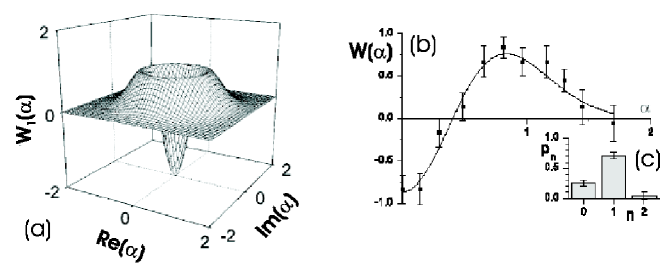
An easier task consists in measuring the value of the Wigner function at the origin of phase space when one knows beforehand that the field in the cavity contains at most one photon. In this case, one does not need to inject a field into the cavity, and the dispersive interaction leading to the phase shift of the field can be replaced by a resonant interaction between levels and (see Fig. 2). This interaction takes the atom from state to state and then back to state (thus the name “-rotation”, in view of the analogy with the full rotation of a spin 1/2), if there is one photon in the field. Exactly as it would happen with a spin 1/2 object, the state changes sign under this transformation: . On the other hand, nothing happens if the atom is in state or if there is no photon in the field. The conditional one-photon phase change is thus accomplished in this case with a resonant interaction, which requires an interaction time much shorter than the dispersive case. This idea was implemented in an experiment at Ecole Normale Supérieure, in Paris Wigner0 . The one-photon state was produced by sending an excited atom through the empty cavity, where the atom suffers a transition, leaving one photon in the cavity, from which it exits in the state . This was the first time a negative value was measured for the Wigner function of an electromagnetic field, namely the value at the origin of the Wigner function corresponding to a one-photon state [this distribution is shown in Fig. 6(a)].
More recently Wigner1 , the Paris group was able to measure the full Wigner function for a one-photon state in the cavity, using the technique proposed in Lutter . The result is displayed in Fig. 6(b), which exhibits a slice of the cylindrically symmetric distribution. From the Wigner function, it is possible to get the photon-number distribution, which is displayed in Fig. 6(c). This distribution shows that the state produced in the cavity is not a perfect one-photon state, which explains the fact that the value of the Wigner function at the origin of phase space is larger than , the value it should have for a one-photon state. An interesting feature of this measurement is that it probes a region of the phase space with area smaller than , which corresponds to the negative region of the Wigner function displayed in Fig. 6. It is thus an explicit demonstration of the fact that it is possible in principle to probe regions of phase space as small as one wants!
5 Conclusion
Since the invention of the laser, the field of quantum optics has been a very active field. Its discoveries have had not only an important technological impact, but have also led to experiments and proposals that probe fundamental questions of quantum mechanics. Some of these questions were discussed here: experiments in the field of cavity quantum electrodynamics have helped us to probe the subtle boundary between the classical and the quantum world, and have allowed the monitoring of the decoherence process, which is at the heart of quantum theory of measurement. The development of new techniques for probing the quantum state of the electromagnetic field in a cavity have led to the experimental unveiling of the Wigner function of a one-photon field, thus demonstrating the feasibility of probing regions of phase space with area smaller than . These methods may lead to a new generation of experiments, which will probe the dynamics of the quantum state of the electromagnetic field.
New challenges involve the demonstration of the teleportation process between two-level atoms telep , as well as trying to control the decoherence process, which is the main villain of quantum computers. Several proposals for fighting decoherence have been made in the last years, ranging from quantum error correction schemes Shor to feedback implementations Mabuchi ; Milburn , from the realization of -bits in symmetric subspaces decoupled from the environment Zanardi to dynamical decoupling techniques Viola and reservoir engineering Luiz4 .
On a fundamental level, difficult problems still persist, related to the classical limit of non-linear systems, where chaotic behavior may play an important role Zurek2 .
Even though fundamental problems related to the classical limit of quantum mechanics and the quantum theory of measurement remain to be solved, I think it is fair to say that quantum optics has helped us to understand and observe an important piece of this puzzle.
Acknowledgments
This work was partially supported by PRONEX (Programa de Apoio a Núcleos de Excelência), CNPq (Conselho Nacional de Desenvolvimento Científico e Tecnológico), FAPERJ (Fundação de Amparo à Pesquisa do Estado do Rio de Janeiro), FUJB (Fundação Universitária José Bonifácio), and the Millennium Institute on Quantum Information. It is a pleasure to acknowledge the collaboration on the subjects covered by this paper with my students A. R. R. Carvalho, M. França Santos, T.B.L. Kist, L.G. Lutterbach, and P. Milman, and with my colleagues M. Brune, S. Haroche, R.L. de Matos Filho, M. Orszag, J.M. Raimond, and N. Zagury.
References
- (1)
- (2) Letter from Albert Einstein to Max Born in 1954, cited by E. Joos, in New Techniques and Ideas in Quantum Measurement Theory, ed. by D. M. Greenberger (New York Academy of Science, New York, 1986).
- (3) E. Schrödinger: Naturwissenschaften 23, 807 (1935); 23, 823 (1935); 23, 844 (1935). English translation by J.D. Trimmer: Proc. Am. Phys. Soc. 124, 3235 (1980).
- (4) J. Von Neumann: Die Mathematische Grundlagen der Quantenmechanik (Springer-Verlag, Berlin, 1932); english translation by R.T. Beyer: Mathematical Foundations of Quantum Mechanics, (Princeton University Press, Princeton, NJ, 1955)
- (5) E. Wigner, in The Scientist Speculates, edited by I.J. Good (William Heinemann, London, 1962), p. 284, and also in Symmetries and Reflections (Indiana University Press, Bloomington, 1967), p. 171. See also E. Wigner: Am. J. of Phys. 31, No. 1 (1963).
- (6) Quantum Theory and Measurement, ed. by J.A. Wheeler and W.H. Zurek (Princeton Univ. Press, Princeton, 1983); W. Zurek: Phys. Today 44, No. 10, 36 (1991); R. Omnès: The Interpretation of Quantum Mechanics (Princeton University Press, Princeton, NJ, 1994); D. Giulini, E. Joos, C. Kiefer, J. Kupsch, I.-O. Stamatescu, and H.D. Zeh: Decoherence and the Appearance of a Classical World in Quantum Theory (Springer, Berlin, 1996).
- (7) K. Hepp: Helv. Phys. Acta 45, 237 (1972); J.S. Bell: Helv. Phys. Acta 48, 93 (1975).
- (8) K. Gottfried: Quantum Mechanics (Benjamim, Reading, MA ,1966), Sec. IV.
- (9) H.D. Zeh: Found. Phys. 1, 69 (1970); W.H. Zurek: Phys. Rev. D 24, 1516 (1981); 26, 1862 (1982); W.G. Unruh and W.H. Zurek: Phys. Rev. D 40, 1071 (1989); W.H. Zurek: Phys. Today 44, No. 10, 36 (1991); B.L. Hu, J.P. Paz, and Y. Zhang: Phys. Rev. D 45, 2843 (1992).
- (10) H. Dekker: Phys. Rev. A 16, 2116 (1977); A.O. Caldeira and A.J. Leggett: Physica (Amsterdam) 121A, 587 (1983); Phys. Rev. A 31, 1059 (1985).
- (11) E. Joos and H.D. Zeh: Z. Phys. B 59, 223 (1985); G.J. Milburn and C.A. Holmes: Phys. Rev. Lett. 56, 2237 (1986); F. Haake and D. Walls: Phys. Rev. A 36, 730 (1987).
- (12) S. Haroche: ‘Cavity Quantum Electrodynamics’. In: Fundamental Systems in Quantum Optics, Proc. Les Houches Summer School, Session LIII, ed. by J. Dalibard, J.M. Raimond, and J. Zinn-Justin (Elsevier, Amsterdam, 1992); see also Cavity Quantum Electrodynamics, ed. by P. Berman (Academic Press, New York, 1994).
- (13) R.J. Glauber: Phys. Rev. 131, 2766-2788, 1963.
- (14) M. Brune, S. Haroche, J.M. Raimond, L. Davidovich, and N. Zagury: Phys. Rev. A 45, 5193 (1992).
- (15) R.G. Hulet and D. Kleppner: Phys. Rev. Lett. 51, 1430 (1983); A. Nussenzveig et al: Euro. Phys. Lett. 14, 755 (1991).
- (16) M. Brune, P. Nussenzveig, F. Schmidt-Kaler, F. Bernardot, A. Maali, J.M. Raimond, and S. Haroche: Phys. Rev. Lett. 76, 1800 (1996).
- (17) J.I. Kim, K.M. Fonseca Romero, A.M. Horiguti, L. Davidovich, M.C. Nemes, and A.F.R. de Toledo Piza: Phys. Rev. Lett. 82, 4737 (1999).
- (18) N.F. Ramsey: Molecular Beams (Oxford Univ. Press, N. Y., 1985).
- (19) A. Einstein, B. Podolski, and N. Rosen: Phys. Rev. 47, 777 (1935).
- (20) J.S. Bell: Physics (Long Island City, N. Y.) 1, 195 (1964).
- (21) S.J. Freedman and J.S. Clauser: Phys. Rev. Lett. 28, 938 (1972); A. Aspect, J. Dalibard, and G. Roger, Phys. Rev. Lett. 49, 1804 (1982).
- (22) M. Brune, E. Hagley, J. Dreyer, X. Maître, A. Maali, C. Wunderlich, J.M. Raimond, and S. Haroche: Phys. Rev. Lett. 77, 4887 (1996).
- (23) L. Davidovich, A. Maali, M. Brune, J.M. Raimond and S. Haroche: Phys. Rev. Lett. 71, 2360 (1993).
- (24) L. Davidovich, M. Brune, J.M. Raimond and S. Haroche: Phys. Rev. A 53, 1295 (1996).
- (25) L.G. Lutterbach and L. Davidovich: Phys. Rev. Lett. 78, 2547 (1997).
- (26) L.G. Lutterbach and L. Davidovich: Optics Express 3, 147 (1998).
- (27) J. Bertrand and P. Bertrand: Found. Phys. 17, 397 (1987).
- (28) U. Leonhardt: Measuring the Quantum State of Light (Cambridge University Press, 1997).
- (29) J. Radon: Berichte über die Verhandlungen der Königlich-Sächsischen Gesellschaft der Wissenschaften zu Leipzig, Mathematisch-Physiche Klass 69, 262 (1917).
- (30) E. Wigner: Phys. Rev. 40, 749 (1932).
- (31) W. Pauli: ‘Die allgemeinen Prinzipien des Wellenmechanik’. In: Handbuch der Physik, ed. by H. Geiger ad K. Scheel (Springer, Berlin, 1933). English translation: W. Pauli: General Principles of Quantum Mechanics (Springer, Berlin, 1980).
- (32) J.E. Moyal: Proc. Cambridge Phil. Soc. 45, 99 (1949).
- (33) K.E. Cahill and R.J. Glauber: Phys. Rev. 177, 1857 (1969); ibid 177, 1882 (1969).
- (34) K. Vogel and H. Risken: Phys. Rev. A 40, 2847 (1989).
- (35) D.T. Smithey, M.Beck, M.G. Raymer and A. Faridani: Phys. Rev. Lett. 70, 1244 (1993).
- (36) G. Breitenbach, T. Müller, S.F. Pereira, J.-Ph. Poizat, S. Schiller and J. Mlynek: J. Opt. Soc. Am. B 12, 2304 (1995).
- (37) T.J. Dunn, I.A. Walmsley, and S. Mukamel: Phys. Rev. Lett. 74, 884 (1995).
- (38) D. Leibfried, D.M. Meekhof, B.E. King, C. Monroe, W.M. Itano and D.J. Wineland: Phys. Rev. Lett. 77, 4281 (1996); see also Physics Today 51, no. 4, 22 (1998).
- (39) L. Davidovich, M. Orszag, and N. Zagury: Phys. Rev. Lett. 57, 2544 (1998).
- (40) G. Nogues, A. Rauschenbeutel, S. Osnaghi, P. Bertet, M. Brune, J.M. Raimond, S. Haroche, L.G. Lutterbach, and L. Davidovich: Phys. Rev. A 62, 054101 (2000).
- (41) P. Bertet, A. Auffeves, P. Maioli, S. Osnaghi, T. Meunier, M. Brune, J.M. Raimond, and S. Haroche, Phys. Rev. Lett. 89, 200402 (2002).
- (42) L. Davidovich, N. Zagury, M. Brune, J.M. Raimond, and S. Haroche: Phys. Rev. A 50, R895 (1994).
- (43) P.W. Shor: Phys. Rev. A 52, 2493 (1995); D. Gottesman: ibid. 54, 1862 (1996); A. Ekert and C. Macchiavello: Phys. Rev. Lett. 77, 2585 (1996); A.R. Calderband et al: ibid. 78, 405 (1997).
- (44) H. Mabuchi and P. Zoller: Phys. Rev. Lett. 76, 3108 (1996).
- (45) D. Vitali, P. Tombesi, and G.J. Milburn: Phys. Rev. Lett. 79, 2442 (1997); Phys. Rev. A 57, 4930 (1998).
- (46) P. Zanardi and M. Rasetti: Phys. Rev. Lett. 79, 3306 (1997); D.A. Lidar, I.L. Chuang, and K.B. Whaley: Phys. Rev. Lett. 81, 2594 (1998); D. Braun, P.A. Braun, and F. Haake: Opt. Comm. 179, 195 (2000).
- (47) L. Viola, E. Knill, and S. Lloyd: Phys. Rev. Lett. 82, 2417 (1999); L. Viola and S. Lloyd: Phys. Rev. A 58, 2733 (1998).
- (48) A.R.R. Carvalho, P. Milman, R.L. de Matos Filho, and L. Davidovich: Phys. Rev. Lett. 86, 4988 (2001).
- (49) W.H. Zurek and J. P. Paz: Phys. Rev. Lett. 72, 2508 (1994); S. Habib, K. Shizume, and W.H. Zurek: Phys. Rev. Lett. 80, 4361 (1998).