Robust quantum information processing with techniques from liquid state NMR

Abstract

quantum logic gate, Nuclear Magnetic Resonance, composite rotation, Ising coupling While Nuclear Magnetic Resonance (NMR) techniques are unlikely to lead to a large scale quantum computer they are well suited to investigating basic phenomena and developing new techniques. Indeed it is likely that many existing NMR techniques will find uses in quantum information processing. Here I describe how the composite rotation (composite pulse) method can be used to develop quantum logic gates which are robust against systematic errors.

1 Introduction

Nuclear Magnetic Resonance (NMR) is arguably both the best technique and the worst technique currently known for implementing quantum information processing. The great strengths and weaknesses of NMR arise from the same fundamental cause: the low frequency of NMR transitions (typically around $500\3\textrm{MHz}$, corresponding to about $2\3\mu\textrm{eV}$). This makes NMR experiments easy to perform (the experimental timescale is conveniently slow), and also acts to minimise the effects of decoherence. However the extreme weakness of NMR signals means that it is not yet possible to study single nuclear spins: instead we must use macroscopic ensembles, which occupy hot thermal states.

These strengths and weaknesses mean that, while it is extremely unlikely that liquid state NMR techniques will ever be used to construct a large scale general purpose quantum computer (Jones 2000), NMR provides an excellent technique for conducting preliminary studies (Cory et al. 1996, 1997; Gershenfeld & Chuang 1997; Jones & Mosca 1998; Chuang et al. 1998), and for developing techniques which will be used in large scale devices. Furthermore, the NMR community has developed a sophisticated library of techniques for manipulating nuclear spins (Ernst et al. 1987; Freeman 1997; Claridge 1999), many of which can be directly transferred to manipulate qubits in other implementations.

In this paper I discuss the method of composite rotations, also called composite pulses (Levitt 1986), which are widely used in NMR to combat systematic errors arising from inevitable experimental imperfections. While many composite pulses developed for use in NMR cannot be directly transferred to quantum computing some can be, and novel composite pulses have been developed specifically for use in quantum computing (Cummins & Jones 2000; Cummins et al. 2002). More recently the concept of composite rotations has been extended to two-qubit (controlled) logic gates (Jones 2002). Although these robust quantum logic gates have been developed in the context of NMR, and are described here using NMR terminology, the basic ideas are entirely general and can be used in many other experimental implementations.

2 Spins, qubits and the Bloch sphere

The majority of conventional NMR studies are conducted on nuclei with spin $I=1/2$, and these also provide a natural method of implementing quantum information processing, as the two spin states, $|\alpha\rangle$ and $|\beta\rangle$, can be trivially mapped to the two basis states of a qubit, $|0\rangle$ and $|1\rangle$. A general superposition state (Nielsen & Chuang 2000) can be written as

$$|\psi\rangle=\cos(\theta/2)|0\rangle+\sin(\theta/2)\re^{i\phi}|1\rangle$$ (1)

(neglecting irrelevant global phases) and so can be thought of as a point on a unit sphere, traditionally called the Bloch sphere, with states $|0\rangle$ and $|1\rangle$ at the north and south poles, and the equally weighted superpositions lying around the equator. Any unitary operation on a single isolated qubit (any single qubit logic gate) corresponds to a rotation of this sphere.

Single qubit rotations can be specified by their rotation axis and their rotation angle; the rotataion axis can itself be described by a single point on the sphere. Within the NMR literature spin states and unitary operations are both described using the product operator notation (Sørensen et al. 1983; Ernst et al. 1987; Hore et al. 2000) . For a single spin

$$\begin{split}|\psi\rangle\langle\psi|&=\frac{1}{2}\left(\textbf{1}+\begin{pmatrix}\cos\theta&\sin\theta\,\re^{-i\phi}\\ \sin\theta\,\re^{i\phi}&-\cos\theta\end{pmatrix}\right)\\ &=\frac{1}{2}\,(\sigma_{0}+\sin\theta\,\cos\phi\,\sigma_{x}+\sin\theta\,\sin\phi\,\sigma_{y}+\cos\theta\,\sigma_{z})\\ &=\mbox{$\frac{1}{2}$}{E}+\sin\theta\,\cos\phi\,I_{x}+\sin\theta\,\sin\phi\,I_{y}+\cos\theta\,I_{z}\end{split}$$ (2)

where the product operators used in the final line are closely related to the corresponding Pauli matrices. NMR systems are usually in hot thermal ensembles, and so are not described by pure states but by highly mixed states (Jones 2001); for a single spin the thermal equilibrium state take the simple form

$$\rho=\textbf{1}+\epsilon I_{z}$$ (3)

It is customary to neglect the 1 term (which cannot be observed by NMR techniques) and the $\epsilon$ factor (which simply determines the signal intensity) and so the equilibrium state is described as $I_{z}$.

3 Pulses and pulse errors

NMR experiments are composed of a series of radiofrequency (RF) pulses, which cause rotations about axes in the $xy$-plane, and periods of free evolution, which for a single spin can be described as $z$ rotations. Two particularly common pulses (Jones 2001) are the $90^{\circ}$ pulse corresponding to excitation

$$I_{z}\xrightarrow{\re^{-i\pi/2\,I_{y}}}I_{x}$$ (4)

(closely related to the Hadamard gate) and the $180^{\circ}$ pulse corresponding to inversion

$$I_{z}\xrightarrow{\re^{-i\pi I_{x}}}-I_{z}$$ (5)

(in effect, a NOT gate). In each case the rotation angle is determined by the applied RF power (which determines the rotation rate) and the length of time over which the RF is applied, while the phase of the rotation axis (in the $xy$ plane) is determined by the phase of the RF field.

Genuine experimental implementations are, of course, not quite as perfect as the description above implies. Clearly a rotation can go wrong in one of two ways: there can be errors in the rotation angle or in the rotation axis. The first type of error, usually called a pulse length error, typically arises when the RF field strength deviates from its assumed value, so that all rotations are systematically too long or too short by some constant fraction. Errors of the second kind, usually called off-resonance effects, occur when the RF field is not exactly in resonance with the transition, resulting in evolution around an effective field, tilted out of the $xy$ plane towards the $\pm z$ axis. The unitary operation describing a real pulse therefore takes the form

$$U=\exp\left(-i\times 2\pi\,\nu\times[(1+g)(I_{x}\,\cos\phi+I_{y}\,\sin\phi)+fI_{z}]\times{t}\right)$$ (6)

where $\nu$ is the nominal rotation rate, $t$ is the pulse length, $\phi$ is the pulse phase, $g$ is the fractional error in the RF power, and $f$ is the off-resonance fraction, given by $f=\delta/\nu$, where $\delta$ is the off-resonance frequency error.

The ideal inversion pulse, equation (5), occurs when $\nu{t}=\pi$, $\phi=0$, and $f=g=0$; in real pulses the last two conditions are relaxed. While both errors can (and do) occur simultaneously, one is typically dominant, and it is most useful to begin by considering these errors separately. Furthermore conventional NMR experiments begin in some well defined initial state, usually $I_{z}$, and the quality of a pulse can be assessed by the overlap between the final state and its ideal form (for an inversion pulse, $-I_{z}$): it is not necessary (or even desirable) to consider the effects of the pulse on other initial states.

In the presence of pulse-length errors, an inversion pulse performs the transformation

$$I_{z}\xrightarrow{\re^{-i\pi(1+g)I_{x}}}-\cos(\pi g)I_{z}+\sin(\pi g)I_{y}$$ (7)

and the component of the final state along the $-I_{z}$ axis, $\cos(\pi g)$, provides a convenient quality measure, lying in the range $\pm 1$. This function is plotted in figure 1; clearly the sequence only performs well for very small values of $g$ (near perfect pulses).

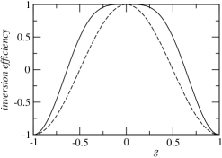
Figure 1: Performance of naive (dashed line) and $90^{\circ}_{y}180^{\circ}_{x}90^{\circ}_{y}$ composite (solid line) inversion pulses in the presence of pulse length errors. Performance is assessed by the component of the final state lying along the $-I_{z}$ axis.

The conventional NMR method for dealing with pulse length errors in inversion pulses is to replace the simple $180^{\circ}_{x}$ pulse with the composite pulse sequence $90^{\circ}_{y}180^{\circ}_{x}90^{\circ}_{y}$. This sequence has an inversion efficiency given by

$$\cos(\pi g)+\mbox{$\frac{1}{2}$}\sin^{2}(\pi g)$$ (8)

which is also plotted in figure 1. The composite sequence performs better than the naive sequence for essentially all values of $g$, but especially for moderate errors, in the range $\pm 10\%$. The manner in which this improvement is achieved can be understood by examining the trajectory on the Bloch sphere in the presence of small errors (Freeman 1997; Claridge 1999).

The situation in the presence of off-resonance effects is more complex, as both the rotation axis and rotation angle are affected. Composite pulse sequences are known which tackle these effects (Levitt 1986), but this point will not be explored further here.

4 Pulses and logic gates

Inversion, which takes $I_{z}$ to $-I_{z}$ is clearly closely related to the NOT gate, which takes $|0\rangle$ to $|1\rangle$, but the two processes are not simply equivalent (Jones 2001). The NOT gate corresponds to a $180^{\circ}$ rotation around the $I_{x}$ axis, while inversion can be achieved by a $180^{\circ}$ rotation around any axis in the $xy$ plane. The difference is that an inversion sequence need only act correctly on the initial states $|0\rangle$ and $|1\rangle$ (corresponding to $I_{z}$ and $-I_{z}$), but a NOT gate must also act correctly on any superposition of these states. In NMR terms this means that the gate must also interchange $I_{y}$ and $-I_{y}$, and must leave $\pm I_{x}$ unchanged. It is, therefore, important to analyse the composite inversion sequence, $90^{\circ}_{y}180^{\circ}_{x}90^{\circ}_{y}$, to see how it performs with these initial states.

In the absence of pulse length errors the composite pulse sequence does, in fact, perform correctly, but in the presence of errors the situation is not so good. While the composite pulse sequence performs better than a simple $180^{\circ}_{x}$ pulse for $\pm I_{z}$ states, it performs worse than the simple sequence for $\pm I_{x}$ states; the effects of the two sequences on $\pm I_{y}$ states are identical. This behaviour is exactly what one might expect: it seems intuitively reasonable that composite pulse sequences should redistribute errors over the Bloch sphere, rather than actually reduce them (Cummins 2001). If this were indeed the case, then composite pulses would have little to offer quantum information processing, but surprisingly some composite pulses are known which perform well for all initial states. Such sequences, sometimes called Class A composite pulses (Levitt 1986), are of little use in conventional NMR, and so have received relatively little study. They are, however, ideally suited to implementing quantum logic gates.

The first application of composite pulses to quantum information processing was by Cummins & Jones (2000), who used composite $90^{\circ}$ pulses to reduce the influence of off-resonance effects on an implementation of quantum counting. More recently Cummins et al. (2002) have described two families of composite pulse sequences which correct for pulse length errors. From here I shall concentrate on one of these, the BB1 sequence originally developed by Wimperis (1994).

5 The BB1 composite pulse sequence

The BB1 composite pulse sequence was developed with two principal aims: firstly to provide good compensation for pulse length errors, and secondly to provide a composite pulse sequence which could be used to replace any simple pulse at any position in a pulse sequence (Wimperis 1994). The second aim is essentially equivalent to seeking a Class A composite pulse, and BB1 does indeed have this property. The first aim is also well achieved by BB1, which provides a quite remarkable degree of compensation for pulse length errors: it is not only better than any other known Class A composite pulse, it can also provide better compensation that many conventional sequences tailored to specific operations (such as inversion).

When assessing the quality of a Class A composite pulse it is necessary to determine how well the unitary transformation actually implemented ($V$) approximates the desired unitary transformation ($U$). A simple and convenient definition of this fidelity is given by

$$\mathcal{F}=\frac{|\text{Tr}(VU^{\dagger})|}{\text{Tr}(UU^{\dagger})}$$ (9)

(note that it is necessary to take the absolute value of the numerator as $U$ and $V$ could in principle differ by an irrelevant global phase shift). A simpler approach, appropriate to single qubit logic gates, is to note that any unitary operation on a single qubit is a rotation, and so can be represented by a quaternion

$$\mathsf{q}=\{s,\mathbf{v}\}$$ (10)

where

$$s=\cos(\theta/2)$$ (11)

depends solely on the rotation angle, $\theta$, and

$$\mathbf{v}=\sin(\theta/2)\mathbf{a}$$ (12)

depends on both the rotation angle, $\theta$, and a unit vector along the rotation axis, $\mathbf{a}$. The quaternion describing a composite pulse sequence is obtained by multiplying the quaternions for each pulse according to the rule

$$\mathsf{q_{1}}\ast\mathsf{q_{2}}=\{s_{1}\cdot s_{2}-\mathbf{v_{1}}\cdot\mathbf{v_{2}},s_{1}\mathbf{v_{2}}+s_{2}\mathbf{v_{1}}+\mathbf{v_{1}}\wedge\mathbf{v_{2}}\}$$ (13)

while two quaternions can be compared using the quaternion fidelity (Levitt 1986)

$$\mathcal{F}(\mathsf{q_{1}},\mathsf{q_{2}})=|\mathsf{q_{1}}\cdot\mathsf{q_{2}}|=|{s_{1}}\cdot{s_{2}}+\mathbf{v_{1}}\cdot\mathbf{v_{2}}|$$ (14)

(it is necessary to take the absolute value, as the two quaternions $\{s,\mathbf{v}\}$ and $\{-s,-\mathbf{v}\}$ correspond to equivalent rotations, differing in their rotation angle by integer multiples of $2\pi$). For single qubit operations the two fidelity definitions (equations 9 and 14) are equivalent, and quaternions will be used from here on.

I shall take as my target operation a NOT gate, that is a $180^{\circ}_{x}$ rotation; similar results can be obtained for any other desired rotation (Wimperis 1994; Cummins et al. 2002). Thus the quaternion representing the ideal operation is

$$\mathsf{q_{0}}=\{0,(1,0,0)\}$$ (15)

while the quaternion representing the rotation which actually occurs (as a result of pulse length errors) is

$$\mathsf{q_{1}}=\{\cos[(1+g)\pi/2],(\sin[(1+g)\pi/2],0,0)\}$$ (16)

giving rise to a quaternion fidelity of

$$\mathcal{F}_{1}=\cos(g\pi/2)\approx 1-\frac{\pi^{2}g^{2}}{8}$$ (17)

(this expression neglects taking the absolute value, and so is only valid for values of $g$ in the range $\pm 100\%$). The conventional composite pulse sequence $90^{\circ}_{y}180^{\circ}_{x}90^{\circ}_{y}$ which has the quaternion form

$$\mathsf{q_{2}}=\{\sin^{2}[g\pi/2],(\cos[g\pi/2],-\sin[g\pi]/2,0)\}$$ (18)

gives exactly the same fidelity, $\mathcal{F}_{2}=\cos(g\pi/2)=\mathcal{F}_{1}$. This confirms that the conventional sequence does not actually correct for errors, but simply redistributes them (Cummins 2001).

One BB1 version of a NOT gate takes the form $90^{\circ}_{0}180^{\circ}_{\phi_{1}}360^{\circ}_{\phi 2}180^{\circ}_{\phi_{1}}90^{\circ}_{0}$, where the phase angles $\phi_{1}$ and $\phi_{2}$ remain to be determined, and a phase angle of $0$ corresponds with an $x$ rotation. Note that this composite pulse sequence comprises a cluster of $180^{\circ}$ and $360^{\circ}$ pulses placed in the middle of a $180^{\circ}_{0}$ pulse. In the absence of errors the central cluster has no effect whatsoever, and the pulse sequence collapses to a simple $180^{\circ}_{0}$ pulse. In the presence of pulse length errors the central cluster will have some effect, and the intention is to choose values of $\phi_{1}$ and $\phi_{2}$ such that the effects of the central cluster compensate the errors in the outer pulses. Note that the sequence discussed here differs subtly from the original BB1 sequence described by Wimperis (1994) which had the cluster placed before the $180^{\circ}_{0}$ pulse; in fact it can be shown that the cluster may be placed at any point with respect to this pulse without affecting the fidelity (Cummins et al. 2002).

The quaternion describing the BB1 composite pulse sequence is complicated. Its $z$ component is zero, as expected for a time-symmetric pulse sequence (Cummins et al. 2002), but the remaining components show a complex dependence on $\phi_{1}$, $\phi_{2}$ and $g$. Progress is most easily made by expanding the quaternion as a Maclaurin series in $g$. The first order $y$ component can be set to 0 by choosing $\phi_{2}=3\phi_{1}$, leaving the approximate quaternion

$$\mathsf{q_{3}}\approx\{-\mbox{$\frac{1}{2}$}\pi[1+4\cos\phi_{1}]g,(1,0,0)\}$$ (19)

(neglecting terms $\textrm{O}(g^{2})$ and higher). Finally the scalar part of $\mathsf{q_{3}}$ can be made approximately equal to 0 by choosing $\phi_{1}=\pm\arccos(-1/4)$, and following previous practice the positive solution is taken. These choices result in a quaternion with a fidelity

$$\mathcal{F}_{3}=\frac{1}{128}\left(150\cos(g\pi/2)-25\cos(3g\pi/2)+3\cos(5g\pi/2)\right)\approx 1-\frac{5\pi^{6}g^{6}}{1024}$$ (20)

in which both the second and fourth order error terms have been cancelled. It is clear from this analysis that the BB1 composite pulse outperforms a simple $180^{\circ}$ pulse for small values of $g$. In fact it does better for all values of $g$ in the range $\pm 100\%$, as shown by the fidelity plots in figure 2; the most spectacular effects are seen within the range $\pm 10\%$, as shown in table 1. BB1 pulses can implement extremely accurate gates in the presence of moderate errors (1–10%), while naive pulses require impossibly accurate control of the RF field strength to achieve the same quality.

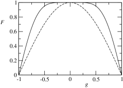
Figure 2: Quaternion fidelity of naive (dashed line) and BB1 composite (solid line) $180^{\circ}_{x}$ pulses used to implement NOT gates in the presence of pulse length errors. The BB1 sequence outperforms a simple pulse for all pulse length errors in the range $\pm 100\%$, and is particularly good in the range $\pm 25\%$.

Table 1: Quaternion infidelities ($1-\mathcal{F}$) of naive and BB1 composite $180^{\circ}_{x}$ pulses.

$g$	naive	BB1
0.1	$1.2\times 10^{-2}$	$4.6\times 10^{-6}$
0.03	$1.1\times 10^{-3}$	$3.4\times 10^{-9}$
0.01	$1.2\times 10^{-4}$	$4.7\times 10^{-12}$
0.003	$1.1\times 10^{-5}$	$3.4\times 10^{-15}$
0.001	$1.2\times 10^{-6}$	$4.7\times 10^{-18}$

It is also instructive to examine the effect of the BB1 pulse on particular initial states. For initial states lying along any of the cardinal axes the BB1 sequence results in an error term of order $g^{6}$, although the exact size of the term depends on the choice of axis. In comparison, for initial states along $\pm I_{z}$ a simple $180^{\circ}_{x}$ pulse results in an error of order $g^{2}$, while the conventional composite pulse sequence, $90^{\circ}_{y}180^{\circ}_{x}90^{\circ}_{y}$, gives an error of order $g^{4}$; thus the BB1 sequence acts as a better inversion sequence than the conventional composite pulse sequence designed to perform an inversion! For initial states along $\pm I_{y}$ the conventional composite pulse sequence provides no compensation, and both it and and the simple pulse give errors of order $g^{2}$. The only blemish on the BB1 sequence is seen when examining initial states along $\pm I_{x}$, for which the simple pulse performs perfectly (the conventional composite pulse gives an error of order $g^{2}$). This property of perfect behaviour along one single axis is a particular property of simple pulses, and cannot be achieved with composite pulses. The very best behaviour for BB1 is observed for initial states along two particular axes in the $xz$ plane, for which an error of order $g^{10}$ is seen.

While the performance of BB1 is extremely impressive, it would obviously be desirable to find an even better sequence, with even better error tolerance. Although such sequences probably exist it is not clear how they can be found. Initial attempts in this direction (G. Llewellyn, unpublished results) have had no success, but have simply made clear how unusually good BB1 actually is.

Very similar composite pulses can be obtained for other pulse angles (Wimperis 1994; Cummins et al. 2002): a $\theta_{0}$ pulse is replaced by $(\theta/2)_{0}180^{\circ}_{\phi}360^{\circ}_{3\phi}180^{\circ}_{\phi}(\theta/2)_{0}$ with $\phi=\arccos(-\theta/4\pi)$. There is, however, a subtle point concerning the accuracy with which such pulse sequences may be implemented. Typically all the pulses in such a sequence are implemented by applying the same RF field for different lengths of time, and the clock controlling the RF field has a finite time resolution. While it is not necessary to control the absolute lengths of each pulse to very great accuracy, it is essential that the relative lengths of each pulse are correct. This is easily achieved when $\theta$ is $180^{\circ}$ or some simple fraction of it, as all the pulses can then be implemented as multiples of some common element, but is much more difficult for arbitrary angles.

6 Two qubit logic gates

It is well known that any desired circuit can be constructed using single qubit logic gates in combination with any one non-trivial two qubit logic gate (Deutsch et al. 1995). The two qubit gate most commonly discussed is the controlled-NOT gate (Barenco et al. 1995) which applies a $180^{\circ}_{x}$ rotation to its target qubit conditional on its control qubit being in the state $|1\rangle$. An essentially equivalent, and frequently more convenient, alternative is the controlled-phase gate, which applies a $180^{\circ}_{z}$ rotation to its target qubit conditional on the state of its control qubit. Note that in this case the logic gate acts symmetrically on the two qubits: the control/target distinction is convenient but artificial. This choice of two qubit gate is particularly convenient in implementations, such as NMR, built around Ising couplings, as the controlled-phase gate and evolution under the Ising coupling are trivially related (Jones 2001, 2002). A controlled-NOT gate can then be implemented by applying Hadamard gates to the target nucleus before and after the controlled-phase gate.

Consider a system of two spin-$1/2$ nuclei, $I$ and $S$. The Ising coupling gate is implemented by evolution under the $J$ coupling Hamiltonian

$$\mathcal{H}_{IS}=\pi J\,2I_{z}S_{z}$$ (21)

for a time $\tau=\phi/\pi J$, where $J$ is the coupling strength and $\phi$ is the desired evolution angle. The desired controlled-phase gate requires $\phi=\pi/2$ and so $\tau=1/2J$; in NMR this is known as the antiphase condition. In order to implement accurate controlled-phase gates it is clearly necessary to know $J$ with corresponding accuracy. This is relatively simple in NMR studies of small molecules, but is much more difficult in larger systems. In particular, many experimental proposals contain an array of qubits coupled by Ising interactions (Ioffe et al. 1999; Cirac & Zoller 2000; Briegel & Raussendorf 2001; Raussendorf & Briegel 2001), with $J$ couplings that are nominally identical but in fact differ from one another as a result of imperfections in the lattice. In systems of this kind it is desirable to be able to perform some accurately known Ising evolution over a range of values of $J$. Perhaps surprisingly, this is relatively easy to achieve using composite pulse techniques.

The problem of performing accurate Ising evolutions is conceptually similar to that of correcting for pulse length errors in single qubit gates, and the solutions are closely related (Jones 2002). Ising coupling corresponds to rotation about the $2I_{z}S_{z}$ axis, and errors in $J$ correspond to errors in the rotation angle about this axis. These can be parameterised by the fractional error in the value of $J$:

$$g=\frac{J_{\textrm{real}}}{J_{\textrm{nominal}}}-1.$$ (22)

Errors of this kind can be overcome by rotating about a sequence of axes tilted from $2I_{z}S_{z}$ towards another axis, such as $2I_{z}S_{x}$. Defining

$$\theta_{\phi}\equiv\exp[-i\times\theta\times(2I_{z}S_{z}\cos\phi+2I_{z}S_{x}\sin\phi)]$$ (23)

allows the direct evolution sequence $(\pi/2)_{0}$ to be replaced by the composite pulse sequence $(\pi/4)_{0}(\pi)_{\phi}(2\pi)_{3\phi}(\pi)_{\phi}(\pi/4)_{0}$ with $\phi=\arccos(-1/8)$. The tilted evolutions can be realised (Ernst et al. 1987) by sandwiching a $2I_{z}S_{z}$ rotation (free evolution under the Ising Hamiltonian) between $\phi_{\mp y}$ pulses applied to spin $S$. After cancellation of extraneous pulses the final sequence takes the form shown in figure 3.

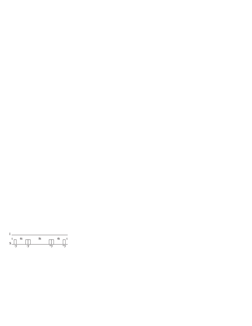
Figure 3: Pulse sequence for a BB1 based robust Ising gate to implement a controlled-phase gate. Boxes correspond to single qubit rotations with rotation angles of $\phi=\arccos(-1/8)\approx 97.2^{\circ}$ applied along the $\pm y$ axes as indicated; time periods correspond to evolution under the Ising coupling, $\pi J\,2I_{z}S_{z}$, for multiples of the time $t=1/4J$. The simple Ising gate corresponds to free evolution for a time $2t$.

Note that the labelling of the two spins as $I$ and $S$ is arbitrary, and the $\phi_{\mp y}$ pulses can be applied to the other spin if this is more convenient.

It is vital that any robust implementation of a quantum logic gate be built from components that are themselves robust. The robust Ising gate uses only two components: single qubit rotations around the $\pm y$ axes, for which robust versions are described above, and periods of evolution under the Ising coupling. As before it is not necessary to accurately control the absolute lengths of the five time periods, but they must have lengths in the integer ratios $1:4:8:4:1$.

The fidelity gain achieved for Ising coupling gates by this approach is identical to that achieved for single qubit rotations. (For two qubit gates it is necessary to use the propagator fidelity, equation 9, but as mentioned above this is equivalent to the quaternion fidelity in the single qubit case). As the controlled-phase gate corresponds to a $90^{\circ}$ rotation, rather than the $180^{\circ}$ rotations discussed in the case of single qubit gates, the fidelities are slightly different from those discussed previously. For a simple Ising gate

$$\mathcal{F}\approx 1-\frac{\pi^{2}g^{2}}{32}$$ (24)

while for a BB1 based robust Ising gate

$$\mathcal{F}\approx 1-\frac{63\pi^{6}g^{6}}{65536}.$$ (25)

The fidelities are plotted in figure 4.

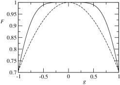
Figure 4: Propagator fidelity of simple (dashed line) and BB1 robust (solid line) Ising gates used to implement controlled-phase gates. The BB1 sequence outperforms a simple gate for errors in the range $\pm 100\%$; over the range $\pm 25\%$ the robust gate is indistinguishable from perfection on this scale.

Clearly the robust Ising gate compensates well for small errors in $J$ values, especially within the range $\pm 25\%$. Over the range $\pm 10\%$ the infidelity of the robust gate is always less that one part in $10^{6}$; to achieve comparable fidelity with a simple gate it is necessary to control $J$ to better than $0.2\%$, more than 50 times more accurately then is needed for the robust gate.

7 Conclusions

Composite rotations show great promise as a method for combatting systematic errors in quantum logic gates. Without progress in this area attempts to build large scale quantum computing devices will founder on the need for impossibly precise experimental control. Methods have been derived for tackling both pulse length errors and off-resonance effects in single qubit gates (Cummins & Jones 2000; Cummins et al. 2002) and for tackling variations in the coupling strength in the Ising coupling two-qubit gate (Jones 2002). Together these provide a universal set of robust quantum logic gates within the Ising coupling model. Although developed within the context of NMR, Ising couplings play a major role in many proposed implementations of quantum information processing (Ioffe et al. 1999; Cirac & Zoller 2000; Briegel & Raussendorf 2001; Raussendorf & Briegel 2001), and these robust gates are likely to find their final applications elsewhere.

- [1] Barenco, A., Bennett, C. H., Cleve, R., DiVincenzo, D. P., Margolus, N., Shor, P., Sleator, T., Smolin, J. A. & Weinfurter, H. 1995 Elementary gates for quantum computation. Phys. Rev. A 52, 3457–3467.
- [2]
- [3] Briegel, H. J. & Raussendorf, R. 2001 Persistent entanglement in arrays of interacting particles. Phys. Rev. Lett. 86, 910–913.
- [4]
- [5] Chuang, I. L., Gershenfeld N. & Kubinec, M. 1998 Experimental implementation of fast quantum searching. Phys. Rev. Lett. 80, 3408–3411.
- [6]
- [7] Cirac, J. I. & Zoller, P. 2000 A scalable quantum computer with ions in an array of microtraps. Nature 404, 579–581.
- [8]
- [9] Claridge, T. D. W. 1999. High-resolution NMR Techniques in organic chemistry. Pergamon, UK.
- [10]
- [11] Cory, D. G., Fahmy, A. & Havel, T. F. 1996 Nuclear magnetic resonance spectroscopy: an experimentally accessible paradigm for quantum computing. In Proc. Phys. Comp. ’96, New England Complex Systems Institute, Boston USA, 22–24 November 1996, pp. 87–91. Reprinted in Quantum computation and quantum information theory (ed. C. Macchiavello, G. M. Palma & A. Zeilinger) World Scientific, Singapore 2001.
- [12]
- [13] Cory, D. G., Fahmy, A. & Havel, T. F. 1997 Ensemble quantum computing by NMR spectroscopy. Proc. Nat. Acad. Sci. USA 94, 1634–1639.
- [14]
- [15] Cummins, H. K. 2001 Quantum information processing and nuclear magnetic resonance. D.Phil. thesis, Oxford University.
- [16]
- [17] Cummins, H. K. & Jones, J. A. 2000 Use of composite rotations to correct systematic errors in NMR quantum computation. New J. Phys. 2, 6 1–12.
- [18]
- [19] Cummins, H. K., Llewellyn, G. & Jones, J. A. 2002 Tackling systematic srrors in quantum logic gates with composite rotations. Submitted to Phys. Rev. A. quant-ph/0208092.
- [20]
- [21] Deutsch, D., Barenco, A. & Ekert, A. 1995 Universality in quantum computation. Proc. Roy. Soc. Lond. A 449, 669–677.
- [22]
- [23] Ernst, R. R., Bodenhausen, G. & Wokaun, A. 1987 Principles of Nuclear Magnetic Resonance in one and two dimensions. Oxford University Press.
- [24]
- [25] Freeman, R. 1997 Spin choreography. Spektrum, Oxford.
- [26]
- [27] Gershenfeld, N. A & Chuang, I. L. 1997 Bulk spin-resonance quantum computation. Science 275, 350–356.
- [28]
- [29] Hore, P. J., Jones, J. A. & Wimperis, S. 2000 NMR: the toolkit. Oxford University Press.
- [30]
- [31] Ioffe, L. B., Geshkenbein, V. B., Feigel’man, M. V., Fauchère, A. L. & Blatter, G. 1999 Environmentally decoupled sds-wave Josephson junctions for quantum computing. Nature 398, 679–681.
- [32]
- [33] Jones, J. A. 2000 NMR quantum computation: a critical evaluation. Fort. Der Physik 48, 909–924.
- [34]
- [35] Jones, J. A. 2001 NMR quantum computation. J. A. Prog. NMR Spectrosc. 38, 325-360.
- [36]
- [37] Jones, J. A. 2002 Robust Ising gates for practical quantum computation. Submitted to Phys. Rev. A. quant-ph/0209049.
- [38]
- [39] Jones, J. A. & Mosca M. 1998 Implementation of a Quantum Algorithm on a Nuclear Magnetic Resonance Quantum Computer. J. Chem. Phys. 109, 1648–1653.
- [40]
- [41] Levitt, M. H. 1986 Composite pulses. Prog. NMR Spectrosc. 18, 61–122.
- [42]
- [43] Nielsen, M. A. & Chuang I. L. 2000 Quantum computation and quantum information. Cambridge University Press.
- [44]
- [45] Raussendorf, R. & Briegel, H. J. 2001 A one-way quantum computer. Phys. Rev. Lett. 86, 5188–5191.
- [46]
- [47] Sørensen, O. W., Eich G. W., Levitt M. H., Bodenhausen G. & Ernst R. R. 1983 Product operator-formalism for the description of NMR pulse experiments. Prog. NMR Spectrosc. 16, 163–192.
- [48]
- [49] Wimperis, S. 1994 Broadband, narrowband, and passband composite pulses for use in advanced NMR experiments. J. Magn. Reson. A 109, 221-231.
- [50]