Macroscopic mechanical oscillators at the quantum limit using optomechanical cooling

Abstract

We discuss how the optomechanical coupling provided by radiation pressure can be used to cool macroscopic collective degrees of freedom, as vibrational modes of movable mirrors. Cooling is achieved using a phase-sensitive feedback-loop which effectively overdamps the mirrors motion without increasing the thermal noise. Feedback results able to bring macroscopic objects down to the quantum limit. In particular, it is possible to achieve squeezing and entanglement.

I Introduction

Radiation pressure is a classical effect which is however at the basis of laser cooling and of many techniques for the manipulation of quantum states of atoms. Its classical origin however naturally suggests to extend its application to a more macroscopic level. In fact, a number of recent papers MVTPRL ; HEIPRL ; PINARD ; ATTO have shown how radiation pressure can be profitably used to cool macroscopic degrees of freedom as, for example, the vibrational modes of a mirror of an optical cavity. The possibility to use optomechanical coupling to cool a cavity mirror in conjunction with a phase-sensitive feedback loop was first pointed out in Ref. MVTPRL . The optomechanical coupling allows one to detect the mirror displacement through a homodyne measurement, and then the output photocurrent can be fed-back in such a way to realize a real-time reduction of the mirror thermal fluctuations. The scheme proposed in Ref. MVTPRL roughly amounts to a continuous version of the stochastic cooling technique used in accelerators ACC . In fact, feedback continuously “kicks” the mirror in order to put it in its equilibrium position, and for this reason the feedback scheme of Ref. MVTPRL has been called “stochastic cooling feedback” in LETTER ; PRALONG . However there are important differences with the scheme used in accelerators and its natural extension in the case of atomic clouds RAIZEN .

A significant improvement has been then achieved with the first experimental realization HEIPRL of the feedback cooling scheme. The experiment however employed a slightly different feedback scheme, the so called “cold damping” technique which was already known in the study of classical electro-mechanical systems COLDD . Cold damping amounts to applying a viscous feedback force to the oscillating mirror. In the experiment of Ref. HEIPRL , the displacement of the mirror is measured with very high sensitivity, and the obtained information is fed back to the mirror via the radiation pressure of another, intensity-modulated, laser beam, incident on the back of the mirror.

The experiment of Ref. HEIPRL has been performed at room temperature, where the effects of quantum noise are blurred by thermal noise and all the results can be well explained in classical terms (see for example PINARD ). However, developing a fully quantum description of the system in the presence of feedback is of fundamental importance, for two main reasons. First of all it allows one to establish the conditions under which the effects of quantum noise in optomechanical systems become visible and experimentally detectable. For example, Ref. LETTER has shown that there is an appreciable difference between the classical and quantum description of feedback already at liquid He temperatures. Moreover, a completely quantum treatment allows one to establish the ultimate limits of the proposed feedback schemes, as for example, the possibility to reach ground state cooling of a mechanical, macroscopic degree of freedom. Quantum limits of feedback cooling have been already discussed in PRALONG ; COURTY , where the possibility to reach ground state cooling has been shown for both schemes. Here we shall review these results and make a detailed comparison of the cooling capabilities of the two different schemes. Morever, the present paper will extend the results of PRALONG for what concerns the possibility to achieve new nonclassical effects in the presence of feedback. In particular we shall see that optomechanical cooling allows purely quantum effects, as squeezing and entanglement, to come out also in macroscopic mechanical oscillators. The experimental realization of these quantum limits in optomechanical systems is extremely difficult, but the feedback methods described in this paper may be useful also for microelectromechanical systems, where the search for quantum effects in mechanical systems is also very active BLENC ; ROUK ; SCHWAB .

The outline of the paper is as follows. In Sec. II we describe the model and derive the appropriate quantum Langevin equations. In Sec. III we describe both feedback schemes using the quantum Langevin theory developed in HOW ; GTV . In Section IV we analyze the stationary state of the system, and we determine the cooling capabilities of both schemes. Section V is devoted to the various nonclassical effects that can be achieved with the feedback scheme of Ref. MVTPRL , while Section VI is for concluding remarks.

II The model

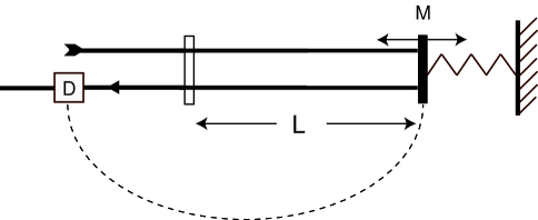
Figure 1: Schematic description of a linear Fabry-Perot cavity with the end oscillating mirror M. The equilibrium cavity length is $L$. A cavity mode is driven by an input laser beam. The output field is subjected to homodyne detection (D). The signal is then fed back to the mirror motion (dashed line).

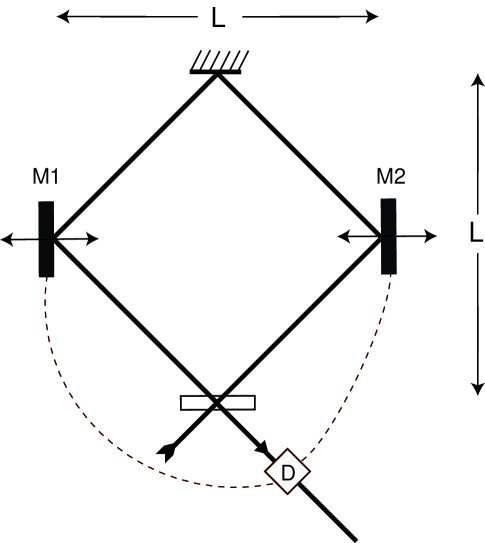
Figure 2: Schematic description of a ring cavity with two oscillating mirrors M1 and M2. The equilibrium distance between them is $L$ (this is also the distance between the fixed mirrors). A cavity mode is driven by an input laser beam. The output field is subjected to homodyne detection (D). The signal is then fed back to the mirrors motion (dashed lines).

We shall consider two examples of optomechanical systems, a Fabry-Perot cavity with an oscillating end mirror (see Fig. 1 for a schematic description), and a ring cavity with two oscillating mirrors (see Fig. 2). These kind of optomechanical systems are used in high sensitivity measurements, as the interferometric detection of gravitational waves GRAV , and in atomic force microscopes AFM . Their ultimate sensitivity is determined by the quantum fluctuations, and therefore each movable mirror has to be described as a single quantum mechanical harmonic oscillator with mass $m$ and frequency $\omega_{m}$. The mirror motion is the result of the excitation of many vibrational modes, including internal acoustic modes. The description of a movable mirror as a single oscillator is however a good approximation when frequencies are limited to a bandwidth including a single mechanical resonance, by using for example a bandpass filter in the detection loop hadjar2 .

The optomechanical coupling between the mirror and the cavity field is realized by the radiation pressure. The electromagnetic field exerts a force on a movable mirror which is proportional to the intensity of the field, which, at the same time, is phase-shifted by an amount proportional to the mirror displacement from its equilibrium position. In the adiabatic limit in which the mirror frequency is much smaller than the cavity free spectral range, one can focus on one cavity mode only, say of frequency $\omega_{c}$, because photon scattering into other modes can be neglected LAW . Moreover, in this adiabatic regime, the generation of photons due to the Casimir effect, and also retardation and Doppler effects are completely negligible HAMI .

Since we shall focus on the quantum and thermal noise of the system, we shall neglect all the technical sources of noise, i.e., we shall assume that the driving laser is stabilized in intensity and frequency. Including these supplementary noise sources is however quite straightforward and a detailed calculation of their effect is shown in Ref. KURT . Moreover recent experiments have shown that classical laser noise can be made negligible in the relevant frequency range HADJAR ; TITTO .

The dynamics of an optomechanical system is also influenced by the dissipative interaction with external degrees of freedom. The cavity mode is damped due to the photon leakage through the mirrors which couple the cavity mode with the continuum of the outside electromagnetic modes. For simplicity we assume that the movable mirrors have perfect reflectivity and that transmission takes place through a “fixed” mirror only. Each mechanical oscillator, which may represent not only the center-of-mass degree of freedom of the mirror, but also a torsional degree of freedom as in TITTO , or an internal acoustic mode as in HADJAR , undergoes Brownian motion caused by the uncontrolled coupling with other internal and external modes at thermal equilibrium.

Let us first analyze the scheme of Fig. 1, which can be described by the following Hamiltonian HAMI

$$H=\hbar\omega_{c}b^{\dagger}b+\hbar\omega_{m}\left(P^{2}+Q^{2}\right)-2\hbar Gb^{\dagger}bQ+i\hbar E\left(b^{\dagger}e^{-i\omega_{0}t}-be^{i\omega_{0}t}\right)\,,$$ (1)

where $b$ is the cavity mode annihilation operator with optical frequency $\omega_{c}$, and $E$ describes the coherent input field with frequency $\omega_{0}\sim\omega_{c}$ driving the cavity. The quantity $E$ is related to the input laser power $\wp$ by $E=\sqrt{\wp\gamma_{c}/\hbar\omega_{0}}$, being $\gamma_{c}$ the photon decay rate. Moreover, $Q$ and $P$ are the dimensionless position and momentum operator of the movable mirror M. It is $\left[Q,P\right]=i/2$, and $G=(\omega_{c}/L)\sqrt{\hbar/2m\omega_{m}}$ represents the optomechanical coupling constant, with $L$ the equilibrium cavity length.

The dynamics of the system can be described by the following set of coupled quantum Langevin equations (QLE) (in the interaction picture with respect to $\hbar\omega_{0}b^{\dagger}b$)

$$\dot{Q}(t) = \omega_{m}P(t)\,,$$ (2)

$$\dot{P}(t) = -\omega_{m}Q(t)+{\cal W}(t)-{\gamma_{m}}P(t)+Gb^{\dagger}(t)b(t)\,,$$ (3)

$$\dot{b}(t) = -\left(i\omega_{c}-i\omega_{0}+\frac{\gamma_{c}}{2}\right)b(t)+2iGQ(t)b(t)+E+\sqrt{\gamma_{c}}b_{in}(t)\,,$$ (4)

where $b_{in}(t)$ is the input noise operator GAR associated with the vacuum fluctuations of the continuum of modes outside the cavity, having the following correlation functions

$$\langle b_{in}(t)b_{in}(t^{\prime})\rangle=\langle b_{in}^{\dagger}(t)b_{in}(t^{\prime})\rangle=0\,,$$ (5)

$$\langle b_{in}(t)b_{in}^{\dagger}(t^{\prime})\rangle=\delta(t-t^{\prime})\,.$$ (6)

Furthermore, ${\cal W}(t)$ is the quantum Langevin force acting on the mirror, with the following correlation function VICTOR ,

$$\langle{\cal W}(t){\cal W}(t^{\prime})\rangle=\frac{1}{2\pi}\frac{\gamma_{m}}{\omega_{m}}\Big{\{}{\cal F}_{r}(t-t^{\prime})+i{\cal F}_{i}(t-t^{\prime})\Big{\}}\,,$$ (7)

where

$${\cal F}_{r}(t) = \int_{0}^{\varpi}d\omega\;\omega\cos(\omega t)\coth\left(\frac{\hbar\omega}{2k_{B}T}\right)\,,$$ (8)

$${\cal F}_{i}(t) = -\int_{0}^{\varpi}d\omega\;\omega\sin(\omega t)\,,$$ (9)

with $T$ the bath temperature, $\gamma_{m}$ the mechanical decay rate, $k_{B}$ the Boltzmann constant, and $\varpi$ the frequency cutoff of the reservoir spectrum. Eqs. (7), (8), and (9) show the non-Markovian nature of quantum Brownian motion, which becomes particularly evident in the low temperature limit GRAB ; HAAKE . The symmetric correlation function becomes proportional to a Dirac delta function when the high temperature limit $k_{B}T\gg\hbar\varpi$ first, and the infinite frequency cutoff limit $\varpi\rightarrow\infty$ later, are taken. It is only in this limit that the exact QLE (2)-(4) reduce to the standard ones GAR . The quantum Langevin description given by Eqs. (2)-(4) is more general than that associated with a master equation approach, which needs a high temperature assumption VICTOR .

In standard applications the driving field is very intense so that the system is characterized by a semiclassical steady state with the internal cavity mode in a coherent state $|\beta\rangle$, and a new equilibrium position for the mirror, displaced by $G|\beta|^{2}/\omega_{m}$ with respect to that with no driving field. The steady state amplitude $\beta$ is given by the solution of the classical nonlinear equation $\beta=E/(\gamma_{c}/2+i\omega_{c}-i\omega_{0}+2iG^{2}/\omega_{m}|\beta|^{2})$. In this case, the dynamics is well described by linearizing the QLE (2)-(4) around the steady state. Redefining with $Q(t)$ and $b(t)$ the quantum fluctuations around the classical steady state, introducing the field phase $Y(t)=i\left(b^{\dagger}(t)-b(t)\right)/2$ and field amplitude $X(t)=\left(b(t)+b^{\dagger}(t)\right)/2$, and choosing the resulting cavity mode detuning $\Delta=\omega_{c}-\omega_{0}+2G^{2}/\omega_{m}\beta^{2}=0$ (by properly tuning the driving field frequency $\omega_{0}$), the linearized QLEs can be rewritten as

$$\dot{Q}(t) = \omega_{m}P(t)\,,$$ (10)

$$\dot{P}(t) = -\omega_{m}Q(t)-{\gamma_{m}}P(t)+2G\beta X(t)+{\cal W}(t)\,,$$ (11)

$$\dot{Y}(t) = -\frac{\gamma_{c}}{2}Y(t)+2G\beta Q(t)+\frac{\sqrt{\gamma_{c}}}{2}Y_{in}(t)\,,$$ (12)

$$\dot{X}(t) = -\frac{\gamma_{c}}{2}X(t)+\frac{\sqrt{\gamma_{c}}}{2}X_{in}(t)\,,$$ (13)

where we have introduced the phase input noise $Y_{in}(t)=i\left(b_{in}^{\dagger}(t)-b_{in}(t)\right)$ and the amplitude input noise $X_{in}(t)=b_{in}^{\dagger}(t)+b_{in}(t)$.

Similar arguments can be used to describe the dynamics of the ring cavity scheme with two movable mirrors of Fig. 2. Assuming for simplicity that the two movable mirrors are identical (i.e., equal mass, frequency and damping), and since the two mirrors are perfectly reflecting, one can easily extend the QLEs for the Fabry-Perot cavity (2)-(4) to the optomechanical system of Fig. 2, and get (in the interaction picture with respect to $\hbar\omega_{0}b^{\dagger}b$)

$$\dot{Q_{1}}(t) = \omega_{m}P_{1}(t)\,,$$ (14)

$$\dot{P_{1}}(t) = -\omega_{m}Q_{1}(t)+{\cal W}_{1}(t)-{\gamma_{m}}P_{1}(t)+{\tilde{G}}b^{\dagger}(t)b(t)\,,$$ (15)

$$\dot{Q_{2}}(t) = \omega_{m}P_{2}(t)\,,$$ (16)

$$\dot{P_{2}}(t) = -\omega_{m}Q_{2}(t)+{\cal W}_{2}(t)-{\gamma_{m}}P_{2}(t)-{\tilde{G}}b^{\dagger}(t)b(t)\,,$$ (17)

$$\dot{b}(t) = -\left(i\omega_{c}-i\omega_{0}+\frac{\gamma_{c}}{2}\right)b(t)+2i{\tilde{G}}\left(Q_{1}(t)-Q_{2}(t)\right)b(t)+E+\sqrt{\gamma_{c}}b_{in}(t)\,,$$ (18)

where $Q_{j}$ and $P_{j}$ $(j=1,\,2)$ are the dimensionless position and momentum operators of the movable mirrors M1 and M2, with $\left[Q_{k},P_{j}\right]=(i/2)\delta_{kj}$, and ${\tilde{G}}=(\omega_{c}/2\sqrt{2}L)\sqrt{\hbar/2m\omega_{m}}$ is the new coupling constant, ($L$ now represents the equilibrium distance between the movable mirrors, as well as the distance between the fixed mirrors, see Fig. 2). The operators ${\cal W}_{1}$ and ${\cal W}_{2}$ are independent Brownian noise operators acting on the mirrors M1 and M2 respectively, each of them with a correlation function specified by Eq. (7).

It is convenient to adopt the center of mass and relative distance coordinates and conjugate momenta, $Q_{\pm}=(Q_{1}\pm Q_{2})/\sqrt{2}$, and $P_{\pm}=(P_{1}\pm P_{2})/\sqrt{2}$. Then, Eqs.(14)-(18) become

$$\dot{Q_{+}}(t) = \omega_{m}P_{+}(t)\,,$$ (19)

$$\dot{P_{+}}(t) = -\omega_{m}Q_{+}(t)+{\cal W}_{+}(t)-{\gamma_{m}}P_{+}(t)\,,$$ (20)

$$\dot{Q_{-}}(t) = \omega_{m}P_{-}(t)\,,$$ (21)

$$\dot{P_{-}}(t) = -\omega_{m}Q_{-}(t)+{\cal W}_{-}(t)-{\gamma_{m}}P_{-}(t)+\sqrt{2}{\tilde{G}}b^{\dagger}(t)b(t)\,,$$ (22)

$$\dot{b}(t) = -\left(i\omega_{c}-i\omega_{0}+\frac{\gamma_{c}}{2}\right)b(t)+2\sqrt{2}i{\tilde{G}}Q_{-}(t)b(t)+E+\sqrt{\gamma_{c}}b_{in}(t)\,,$$ (23)

where ${\cal W}_{\pm}=({\cal W}_{1}\pm{\cal W}_{2})/\sqrt{2}$ are again independent Brownian noise operators. It is evident from these equations that only the relative motion of the two mrrors is coupled to the radiation field, while the center of mass undergoes a simple Brownian motion. Thus, neglecting the latter, the QLEs for the dynamics of the relative motion and the cavity mode are identical to those of the single mirror case, Eqs. (2)-(4), except for the replacements $Q\to Q_{-}$, $P\to P_{-}$, and $G\to\sqrt{2}{\tilde{G}}$. One can again consider an intensely driven cavity mode, and the fluctuations around the semiclassical steady state, as discussed above in the Fabry-Perot case. One has a consequently modified steady state coherent amplitude $\tilde{\beta}$, and the linearized equations for the relative motion and the cavity mode (assuming again zero cavity mode detuning) become identical to those of the Fabry-Perot case, Eqs. (10)-(13), with the corresponding replacements $Q\to Q_{-}$, $P\to P_{-}$, $\beta\to\tilde{\beta}$, and $G\to\sqrt{2}\tilde{G}$.

III Position measurement and feedback

As it is shown by Eq. (12), when the driving and the cavity fields are resonant, the dynamics is simpler because only the phase quadrature $Y(t)$ is affected by the mirror position fluctuations $Q(t)$, while the amplitude quadrature $X(t)$ is not. Therefore the mechanical motion of the mirror can be detected by monitoring the phase quadrature $Y(t)$. In the ring cavity case, the phase quadrature $Y(t)$ instead reproduces the relative motion dynamics. However, to fix the ideas, we shall focus for simplicity onto the Fabry-Perot cavity case only. The mirror position measurement is commonly performed in the large cavity bandwidth limit $\gamma_{c}\gg G\beta$, $\omega_{m}$, when the cavity mode dynamics adiabatically follows that of the movable mirror and it can be eliminated, that is, from Eq. (12),

$$Y(t)\simeq\frac{4G\beta}{\gamma_{c}}Q(t)+\frac{Y_{in}(t)}{\sqrt{\gamma_{c}}},$$ (24)

and $X(t)\simeq X_{in}(t)/\sqrt{\gamma_{c}}$ from Eq. (13). The experimentally detected quantity is the output homodyne photocurrent HOW ; GTV ; homo

$$Y_{out}(t)=2\eta\sqrt{\gamma_{c}}Y(t)-\sqrt{\eta}Y_{in}^{\eta}(t)\,,$$ (25)

where $\eta$ is the detection efficiency and $Y_{in}^{\eta}(t)$ is a generalized phase input noise, coinciding with the input noise $Y_{in}(t)$ in the case of perfect detection $\eta=1$, and taking into account the additional noise due to the inefficient detection in the general case $\eta<1$ GTV . This generalized phase input noise can be written in terms of a generalized input noise $b_{\eta}(t)$ as $Y_{in}^{\eta}(t)=i\left[b_{\eta}^{\dagger}(t)-b_{\eta}(t)\right]$. The quantum noise $b_{\eta}(t)$ is correlated with the input noise $b_{in}(t)$ and it is characterized by the following correlation functions GTV

$$\langle b_{\eta}(t)b_{\eta}(t^{\prime})\rangle=\langle b_{\eta}^{\dagger}(t)b_{\eta}(t^{\prime})\rangle=0\,,$$ (26)

$$\langle b_{\eta}(t)b_{\eta}^{\dagger}(t^{\prime})\rangle=\delta(t-t^{\prime})\,,$$ (27)

$$\langle b_{in}(t)b_{\eta}^{\dagger}(t^{\prime})\rangle=\langle b_{\eta}(t)b_{in}^{\dagger}(t^{\prime})\rangle=\sqrt{\eta}\delta(t-t^{\prime}).$$ (28)

The output of the homodyne measurement may be used to devise a phase-sensitive feedback loop to control the dynamics of the mirror, as it has been done in Ref. MVTPRL , and in Refs. HEIPRL ; PINARD using cold damping. Let us now see in detail how these two feedback schemes modify the quantum dynamics of the mirror.

In the scheme of Ref. MVTPRL , the feedback loop induces a continuous position shift controlled by the output homodyne photocurrent $Y_{out}(t)$. This effect of feedback manifests itself in an additional term in the QLE for a generic operator ${\cal O}(t)$ given by

$$\dot{{\cal O}}_{fb}(t)=i\frac{\sqrt{\gamma_{c}}}{\eta}\int_{0}^{t}dt^{\prime}G_{mf}(t^{\prime})Y_{out}(t-t^{\prime})\left[g_{mf}P(t),{\cal O}(t)\right]\,,$$ (29)

where $G_{mf}(t)$ is the feedback transfer function, and $g_{mf}$ is a feedback gain factor. The implementation of this scheme is nontrivial because it is equivalent to add a feedback interaction linear in the mirror momentum, as it could be obtained with a charged mirror in a homogeneous magnetic field. For this reason here we shall refer to it as “momentum feedback” (see, however, the recent parametric cooling scheme demonstrated in Ref. ATTO , showing some similarity with the feedback scheme of Ref. MVTPRL ).

Feedback is characterized by a delay time which is essentially determined by the electronics and is always much smaller than the typical timescale of the mirror dynamics. It is therefore common to consider the zero delay-time limit $G_{mf}(t)\sim\delta(t)$, which is quite delicate in general HOW ; GTV . However, for linearized systems, the limit can be taken directly in Eq. (29) PRALONG , so to get the following QLE in the presence of feedback

$$\dot{Q}(t) = \omega_{m}P(t)+g_{mf}\gamma_{c}Y(t)-\frac{g_{mf}}{2}\sqrt{\frac{\gamma_{c}}{\eta}}Y_{in}^{\eta}(t)\,,$$ (30)

$$\dot{P}(t) = -\omega_{m}Q(t)-{\gamma_{m}}P(t)+2G\beta X(t)+{\cal W}(t)\,,$$ (31)

$$\dot{Y}(t) = -\frac{\gamma_{c}}{2}Y(t)+2G\beta Q(t)+\frac{\sqrt{\gamma_{c}}}{2}Y_{in}(t)\,,$$ (32)

$$\dot{X}(t) = -\frac{\gamma_{c}}{2}X(t)+\frac{\sqrt{\gamma_{c}}}{2}X_{in}(t)\,,$$ (33)

where we have used Eq. (25). After the adiabatic elimination of the radiation mode (see Eq. (24)), and introducing the rescaled, dimensionless, input power of the driving laser

$$\zeta=\frac{16G^{2}\beta^{2}}{\gamma_{m}\gamma_{c}}=\frac{64G^{2}}{\hbar\omega_{0}\gamma_{m}\gamma_{c}^{2}}\wp,$$ (34)

and the rescaled feedback gain $g_{1}=-4G\beta g_{mf}/\gamma_{m}$, the above equations reduce to

$$\dot{Q}(t) = \omega_{m}P(t)-\gamma_{m}g_{1}Q(t)-\sqrt{\frac{\gamma_{m}}{\zeta}}g_{1}Y_{in}(t)+\sqrt{\frac{\gamma_{m}}{\eta\zeta}}\frac{g_{1}}{2}Y_{in}^{\eta}(t)\,,$$ (35)

$$\dot{P}(t) = -\omega_{m}Q(t)-\gamma_{m}P(t)+\frac{1}{2}\sqrt{\gamma_{m}\zeta}X_{in}(t)+{\cal W}(t)\,.$$ (36)

This treatment explicitly includes the limitations due to the quantum efficiency of the detection, but neglects other possible technical imperfections of the feedback loop, as for example the electronic noise of the feedback loop, whose effects have been discussed in PINARD .

Cold damping techniques have been applied in classical electromechanical systems for many years COLDD , and only recently they have been proposed to improve cooling and sensitivity at the quantum level GRAS . This technique is based on the application of a negative derivative feedback, which increases the damping of the system without correspondingly increasing the thermal noise COLDD ; GRAS . This technique has been succesfully applied for the first time to an optomechanical system composed of a high-finesse cavity with a movable mirror in the experiments of Refs. HEIPRL ; PINARD ; ATTO . In these experiments, the displacement of the mirror is measured with very high sensitivity ATTO ; HADJAR , and the obtained information is fed back to the mirror via the radiation pressure of another, intensity-modulated, laser beam, incident on the back of the mirror. Cold damping is obtained by modulating with the time derivative of the homodyne signal, in such a way that the radiation pressure force is proportional to the mirror velocity. The results of Refs. HEIPRL ; PINARD ; ATTO referred to a room temperature experiment, and have been explained using a classical description. The quantum description of cold damping has been instead presented in GRAS using quantum network theory, and in PRALONG ; LETTER using a quantum Langevin description. In this latter treatment, cold damping implies the following additional term in the QLE for a generic operator ${\cal O}(t)$,

$$\dot{{\cal O}}_{fb}(t)=\frac{i}{\eta\sqrt{\gamma_{c}}}\int_{0}^{t}dt^{\prime}G_{cd}(t^{\prime})Y_{out}(t-t^{\prime})\left[g_{cd}Q(t),{\cal O}(t)\right]\,.$$ (37)

As in the previous case, one usually assume a Markovian feedback loop with negligible delay. Since one needs a derivative feedback, this would ideally imply $G_{cd}(t)=-\delta^{\prime}(t)$, i.e., $\tilde{G}_{cd}(\omega)=i\omega$, $\forall\omega$, even though, in practice, it is sufficient to satisfy this condition within the detection bandwidth $\Delta\omega$. In this case, the QLEs for the cold damping feedback scheme become

$$\dot{Q}(t) = \omega_{m}P(t)\,,$$ (38)

$$\dot{P}(t) = -\omega_{m}Q(t)-{\gamma_{m}}P(t)+2G\beta X(t)-g_{cd}\dot{Y}(t)+\frac{g_{cd}}{2\sqrt{\gamma_{c}\eta}}\dot{Y}_{in}^{\eta}(t)+{\cal W}(t)\,,$$ (39)

$$\dot{Y}(t) = -\frac{\gamma_{c}}{2}Y(t)+2G\beta Q(t)+\frac{\sqrt{\gamma_{c}}}{2}Y_{in}(t)\,,$$ (40)

$$\dot{X}(t) = -\frac{\gamma_{c}}{2}X(t)+\frac{\sqrt{\gamma_{c}}}{2}X_{in}(t)\,.$$ (41)

Adiabatically eliminating the cavity mode, and introducing the rescaled, dimensionless feedback gain $g_{2}=4G\beta\omega_{m}g_{cd}/\gamma_{m}\gamma_{c}$, one has

$$\dot{Q}(t)=\omega_{m}P(t),$$ (42)

$$\dot{P}(t)=-\omega_{m}Q(t)-{\gamma_{m}}P(t)+\frac{1}{2}\sqrt{\gamma_{m}\zeta}X_{in}(t)+{\cal W}(t)$$

$$-\frac{\gamma_{m}g_{2}}{\omega_{m}}\dot{Q}(t)-\frac{g_{2}\sqrt{\gamma_{m}}}{\omega_{m}\sqrt{\zeta}}\dot{Y}_{in}(t)+\frac{g_{2}\sqrt{\gamma_{m}}}{2\omega_{m}\sqrt{\eta\zeta}}\dot{Y}_{in}^{\eta}(t).$$ (43)

The presence of an ideal derivative feedback implies the introduction of two new quantum input noises, $\dot{Y}_{in}(t)$ and $\dot{Y}_{in}^{\eta}(t)$, whose correlation functions can be simply obtained by differentiating the corresponding correlation functions of $Y_{in}(t)$ and $Y_{in}^{\eta}(t)$. We have therefore

$$\langle\dot{Y}_{in}(t)\dot{Y}_{in}(t^{\prime})\rangle = \langle\dot{Y}_{in}(t^{\prime})\dot{Y}_{in}(t)\rangle=\langle\dot{Y}_{in}^{\eta}(t)\dot{Y}_{in}^{\eta}(t^{\prime})\rangle=\langle\dot{Y}_{in}^{\eta}(t^{\prime})\dot{Y}_{in}^{\eta}(t)\rangle=-\ddot{\delta}(t-t^{\prime}),$$ (44)

$$\langle\dot{Y}_{in}^{\eta}(t)\dot{Y}_{in}(t^{\prime})\rangle = \langle\dot{Y}_{in}(t^{\prime})\dot{Y}_{in}^{\eta}(t)\rangle=-\sqrt{\eta}\ddot{\delta}(t-t^{\prime}),$$ (45)

$$\langle X_{in}(t)\dot{Y}_{in}^{\eta}(t^{\prime})\rangle = -\langle\dot{Y}_{in}^{\eta}(t^{\prime})X_{in}(t)\rangle=-i\sqrt{\eta}\dot{\delta}(t-t^{\prime}),$$ (46)

which however, as discussed above, have to be considered as approximate expressions valid within the detection bandwidth only.

The two sets of QLE for the mirror Heisenberg operators, Eqs. (35)-(36) and (42)-(43), show that the two feedback schemes are not exactly equivalent. They are however physically analogous, as it can be seen, for example, by looking at the differential equation for the displacement operator $Q(t)$. In fact, from Eqs. (35) and (36) one gets

$$\ddot{Q}(t)+\left(1+g_{1}\right)\gamma_{m}\dot{Q}(t)+\left(\omega_{m}^{2}+\gamma_{m}^{2}g_{1}\right)Q(t)$$

$$=\omega_{m}\left[\frac{1}{2}\sqrt{\gamma_{m}\zeta}X_{in}(t)+{\cal W}(t)\right]-\sqrt{\frac{\gamma_{m}}{\zeta}}g_{1}\left(\dot{Y}_{in}(t)+\gamma_{m}Y_{in}(t)\right)$$ (47)

$$+\sqrt{\frac{\gamma_{m}}{\eta\zeta}}\frac{g_{1}}{2}\left(\dot{Y}_{in}^{\eta}(t)+\gamma_{m}Y_{in}^{\eta}(t)\right),$$

for the momentum feedback scheme, while from Eqs. (42) and (43) one gets

$$\ddot{Q}(t)+\left(1+g_{2}\right)\gamma_{m}\dot{Q}(t)+\omega_{m}^{2}Q(t)$$ (48)

$$=\omega_{m}\left[\frac{1}{2}\sqrt{\gamma_{m}\zeta}X_{in}(t)+{\cal W}(t)-\frac{g_{2}\sqrt{\gamma_{m}}}{\omega_{m}\sqrt{\zeta}}\dot{Y}_{in}(t)+\frac{g_{2}\sqrt{\gamma_{m}}}{2\omega_{m}\sqrt{\eta\zeta}}\dot{Y}_{in}^{\eta}(t)\right],$$

for the cold damping scheme. The comparison shows that in both schemes the main effect of feedback is the modification of mechanical damping $\gamma_{m}\rightarrow\gamma_{m}(1+g_{i})$ ($i=1,2$). In the momentum feedback scheme one has also a frequency renormalization $\omega_{m}^{2}\rightarrow\omega_{m}^{2}+\gamma_{m}^{2}g_{1}$, which is however negligible when the mechanical quality factor ${\cal Q}=\omega_{m}/\gamma_{m}$ is large. Moreover, the noise terms are similar, but not identical. In particular, the feedback scheme of Ref. MVTPRL is also subject to the phase noises $Y_{in}(t)$ and $Y_{in}^{\eta}(t)$, while cold damping is not. However, the comparison shows that also momentum feedback provides a cold damping effect of increased damping without an increased temperature.

IV Cooling and stationary state

We now study the stationary state of the movable mirror in the presence of both feedback schemes, which is obtained by considering the dynamics in the asymptotic limit $t\to\infty$. We shall see that, in both cases, ground state cooling can be achieved.

IV.1 Cold damping

Now we characterize the stationary state of the mirror in the presence of cold damping. This stationary state has been already studied using classical arguments in HEIPRL ; PINARD , while the discussion of the cooling limits of cold damping in the quantum case has been recently presented in COURTY . The results of COURTY have been generalized to the case of nonideal quantum efficiency $\eta<1$ in PRALONG , and here we shall review these results and compare in detail the cooling capabilities of the two feedback schemes.

The stationary variances can be expressed in terms of the Fourier transforms of the noise correlation functions, and using the correlation functions (5), (6), (7), (26)-(28), and (44)-(46), one can write

$$\langle Q^{2}\rangle_{st} = \gamma_{m}\int_{-\infty}^{\infty}\frac{d\omega}{2\pi}\left|{\tilde{\chi}}_{cd}(\omega)\right|^{2}\left[\frac{\zeta}{4}+\frac{g_{2}^{2}}{4\eta\zeta}\frac{|\tilde{G}_{cd}(\omega)|^{2}}{\omega_{m}^{2}}\right.$$ (49)

$$\left.+\frac{\omega}{2\omega_{m}}\coth\left(\frac{\hbar\omega}{2k_{B}T}\right)\Theta_{[-\varpi,\varpi]}(\omega)\right],$$

$$\langle P^{2}\rangle_{st} = \gamma_{m}\int_{-\infty}^{\infty}\frac{d\omega}{2\pi}\frac{\omega^{2}}{\omega_{m}^{2}}\left|{\tilde{\chi}}_{cd}(\omega)\right|^{2}\left[\frac{\zeta}{4}+\frac{g_{2}^{2}}{4\eta\zeta}\frac{|\tilde{G}_{cd}(\omega)|^{2}}{\omega_{m}^{2}}\right.$$ (50)

$$\left.+\frac{\omega}{2\omega_{m}}\coth\left(\frac{\hbar\omega}{2k_{B}T}\right)\Theta_{[-\varpi,\varpi]}(\omega)\right],$$

where

$${\tilde{\chi}}_{cd}(\omega)=\frac{\omega_{m}}{\omega_{m}^{2}-\omega^{2}+i\omega\gamma_{m}\left(1+g_{2}\right)}$$ (51)

is the frequency-dependent susceptibility of the mirror in the cold damping feedback scheme, and $\Theta_{[-\varpi,\varpi]}(\omega)$ is a gate function equal to 1 for $|\omega|<\varpi$ and zero otherwise.

In general, each steady state variance has three contributions: i) the back action of the radiation pressure, proportional to the input power $\zeta$; ii) the feedback-induced noise term proportional to the feedback gain squared, and inversely proportional to the input power; iii) the thermal noise term due to the mirror Brownian motion. The back-action contribution can be evaluated in a straightforward way for both variances, and it is given by

$$\langle Q^{2}\rangle_{st}^{ba}=\langle P^{2}\rangle_{st}^{ba}=\frac{\zeta}{8(1+g_{2})}.$$ (52)

The feedback-induced contribution generally depends upon the form of $|\tilde{G}_{cd}(\omega)|^{2}$, where $\tilde{G}_{cd}(\omega)$ is a causal function (i.e., it is analytic for ${\rm Im}\omega<0$) and approximatively equal to $i\omega$ within the detection bandwidth $\Delta\omega$. The factor $|{\tilde{\chi}}_{cd}(\omega)|^{2}$ is highly peaked around the mechanical resonance $\omega=\omega_{m}$, with width $\gamma_{m}(1+g_{2})$. Since it is usually $\gamma_{m}(1+g_{2})<\Delta\omega$, one can safely approximate $|\tilde{G}_{cd}(\omega)|^{2}$ with its value at the resonance peak, $|\tilde{G}_{cd}(\omega)|^{2}\simeq\omega_{m}^{2}$, and obtain

$$\langle Q^{2}\rangle_{st}^{fb}=\langle P^{2}\rangle_{st}^{fb}=\frac{g_{2}^{2}}{8\eta\zeta(1+g_{2})}.$$ (53)

The Brownian motion contribution is generally cumbersome and it has been already exactly evaluated for both variances in GRAB . However, in optomechanical systems, the condition $\hbar\omega_{m}\ll k_{B}T$ is commonly met, and the classical approximation $\coth(\hbar\omega/2k_{B}T)\simeq 2k_{B}T/\hbar\omega$ can be made in the expression for $\langle Q^{2}\rangle_{st}$, obtaining

$$\langle Q^{2}\rangle_{st}^{BM}=\frac{k_{B}T}{2\hbar\omega_{m}(1+g_{2})}.$$ (54)

In the evaluation of $\langle P^{2}\rangle_{st}^{BM}$ instead, the classical approximation has to be made with care, because, due to the presence of the $\omega^{2}$ term, the integral (50) has an ultraviolet divergence in the usually considered $\varpi\to\infty$ limit (see also Eq. (51)). This means that, differently from $\langle Q^{2}\rangle_{st}^{BM}$, the classical approximation for $\langle P^{2}\rangle_{st}^{BM}$ is valid only under the stronger condition $\hbar\varpi\ll k_{B}T$ GRAB , and that in the intermediate temperature range $\hbar\varpi\gg k_{B}T\gg\hbar\omega_{m}$ (which may be of interest for optomechanical systems), one has an additional logarithmic correction, so to get

$$\langle P^{2}\rangle_{st}^{BM}=\frac{k_{B}T}{2\hbar\omega_{m}}\frac{1}{1+g_{2}}+\frac{\gamma_{m}}{\pi\omega_{m}}\ln\left(\frac{\hbar\varpi}{2\pi kT}\right).$$ (55)

However, in the common situation of a high ${\cal Q}$ mechanical mode, this logarithmic correction can be neglected, the dependence on the frequency cutoff $\varpi$ vanishes, and one finally gets

$$\langle Q^{2}\rangle_{st}=\langle P^{2}\rangle_{st}=\left[\frac{g_{2}^{2}}{8\eta\zeta}+\frac{\zeta}{8}+\frac{k_{B}T}{2\hbar\omega_{m}}\right]\frac{1}{1+g_{2}}.$$ (56)

This fact, together with the fact that

$$\langle PQ+QP\rangle_{st}=\frac{1}{\omega_{m}}\lim_{t\to\infty}\frac{d}{dt}\langle Q(t)^{2}\rangle=0,$$ (57)

implies that the stationary state in the presence of cold damping is an effective thermal state with a mean excitation number $\langle n\rangle=2\langle Q^{2}\rangle_{st}-1/2$, where $\langle Q^{2}\rangle_{st}$ is given by Eq. (56). This effective thermal equilibrium state in the presence of cold damping has been already pointed out in HEIPRL ; PINARD , within a classical treatment neglecting both the back-action and the feedback-induced terms. The present fully quantum analysis shows that cold damping has two opposite effects on the effective equilibrium temperature of the mechanical mode: on one hand $T$ is reduced by the factor $(1+g_{2})^{-1}$, but, on the other hand, the effective temperature is increased by the additional noise terms.

Let us now consider the optimal conditions for cooling, and the cooling limits of the cold damping feedback scheme. Neglecting the logarithmic correction to $\langle P^{2}\rangle_{st}^{BM}$, the stationary oscillator energy is given by

$$U_{st}=2\hbar\omega_{m}\langle Q^{2}\rangle_{st}=\frac{\hbar\omega_{m}}{4\left(1+g_{2}\right)}\left[\frac{g_{2}^{2}}{\eta\zeta}+\zeta+\frac{4k_{B}T}{\hbar\omega_{m}}\right].$$ (58)

This expression coincides with that derived and discussed in COURTY , except for the presence of the homodyne detection efficiency $\eta$, which was ideally assumed equal to one in COURTY . The optimal conditions for cooling can be derived in the same way as it has been done in COURTY . The energy $U_{st}$ is minimized with respect to $\zeta$ keeping $g_{2}$ fixed, thereby getting $\zeta_{opt}=g_{2}/\sqrt{\eta}$. Under these conditions, the stationary oscillator energy becomes

$$U_{st}=\frac{\hbar\omega_{m}}{2}\frac{g_{2}}{1+g_{2}}\left[\frac{1}{\sqrt{\eta}}+\frac{2k_{B}T}{\hbar\omega_{m}}\frac{1}{g_{2}}\right]\;,$$ (59)

showing that, in the ideal limit $\eta=1$, $g_{2}\to\infty$ (and therefore $\zeta\sim g_{2}\to\infty$), cold damping is able to reach the quantum limit $U_{st}=\hbar\omega_{m}/2$, i.e., it is able to cool the mirror to its quantum ground state, as first pointed out in COURTY .

Fig. 3 shows the rescaled steady-state energy $2U_{st}/\hbar\omega_{m}$ versus $\zeta$ plotted for increasing values of $g_{2}$ (a: $g_{2}=10$, b: $g_{2}=10^{3}$, c: $g_{2}=10^{5}$, d: $g_{2}=10^{7}$), with $k_{B}T/\hbar\omega_{m}=10^{5}$ and $\eta=0.8$. For high gain values, ground state cooling can be achieved, even with nonunit homodyne detection efficiency.

IV.2 Momentum feedback

One can proceed in a similar manner for the evaluation of the steady-state variances in the case of the feedback of Ref. MVTPRL . One has again the back-action, the feedback-induced, and the Brownian motion contributions. Differently from cold damping however, the variances now strongly depend on the mechanical quality factor ${\cal Q}$ and each noise contributes differently to $\langle Q^{2}\rangle_{st}$ and $\langle P^{2}\rangle_{st}$. In the Markovian, zero-delay limit it is $\tilde{G}_{mf}(\omega)=1$, and the feedback-induced noise is delta-correlated as the back-action noise. Using the correlation functions (5), (6), (7), and (26)-(28), one arrives at PRALONG

$$\langle Q^{2}\rangle_{st}^{ba} = \frac{\zeta{\cal Q}^{2}}{8\left(1+g_{1}\right)\left({\cal Q}^{2}+g_{1}\right)},$$ (60)

$$\langle P^{2}\rangle_{st}^{ba} = \frac{\zeta\left({\cal Q}^{2}+g_{1}^{2}+g_{1}\right)}{8\left(1+g_{1}\right)\left({\cal Q}^{2}+g_{1}\right)},$$ (61)

for the back-action contribution, and

$$\langle Q^{2}\rangle_{st}^{fb} = \frac{g_{1}^{2}}{8\eta\zeta}\frac{1+{\cal Q}^{2}+g_{1}}{\left(1+g_{1}\right)\left({\cal Q}^{2}+g_{1}\right)},$$ (62)

$$\langle P^{2}\rangle_{st}^{fb} = \frac{g_{1}^{2}}{8\eta\zeta}\frac{{\cal Q}^{2}}{\left(1+g_{1}\right)\left({\cal Q}^{2}+g_{1}\right)},$$ (63)

for the feedback-induced contribution.

Finally, for the Brownian motion contribution, one has a situation analogous to that discussed for the cold damping scheme. The generally valid expressions for the variances have been already exactly evaluated in GRAB . However, in the limit $\hbar\omega_{m}\ll k_{B}T$, we can make the classical approximation $\coth(\hbar\omega/2k_{B}T)\simeq 2k_{B}T/\hbar\omega$ in the expression for $\langle Q^{2}\rangle_{st}$, obtaining

$$\langle Q^{2}\rangle_{st}^{BM}=\frac{k_{B}T}{2\hbar\omega_{m}}\frac{{\cal Q}^{2}}{(1+g_{2})({\cal Q}^{2}+g_{1})}.$$ (64)

Also in this feedback scheme, the Brownian motion contribution to $\langle P^{2}\rangle_{st}$ has an ultraviolet divergence in the usually considered $\varpi\to\infty$ limit PRALONG . Again, the classical approximation for $\langle P^{2}\rangle_{st}^{BM}$ is valid only under the stronger condition $\hbar\varpi\ll k_{B}T$ GRAB , and, in the intermediate temperature range $\hbar\varpi\gg k_{B}T\gg\hbar\omega_{m}$, one has an additional logarithmic correction, i.e.,

$$\langle P^{2}\rangle_{BM}=\frac{k_{B}T}{2\hbar\omega_{m}}\frac{g_{1}^{2}+{\cal Q}^{2}+g_{1}}{\left(1+g_{1}\right)\left({\cal Q}^{2}+g_{1}\right)}+\frac{\gamma_{m}}{\pi\omega_{m}}\ln\left(\frac{\hbar\varpi}{2\pi kT}\right).$$ (65)

Summing up the three contributions, we arrive at PRALONG

$$\langle Q^{2}\rangle_{st} = \frac{g_{1}^{2}}{8\eta\zeta}\frac{1+{\cal Q}^{2}+g_{1}}{\left(1+g_{1}\right)\left({\cal Q}^{2}+g_{1}\right)}+\left[\frac{\zeta}{8}+\frac{k_{B}T}{2\hbar\omega_{m}}\right]\frac{{\cal Q}^{2}}{\left(1+g_{1}\right)\left({\cal Q}^{2}+g_{1}\right)},$$ (66)

$$\langle P^{2}\rangle_{st} = \frac{g_{1}^{2}}{8\eta\zeta}\frac{{\cal Q}^{2}}{\left(1+g_{1}\right)\left({\cal Q}^{2}+g_{1}\right)}+\left[\frac{\zeta}{8}+\frac{k_{B}T}{2\hbar\omega_{m}}\right]\frac{g_{1}^{2}+{\cal Q}^{2}+g_{1}}{\left(1+g_{1}\right)\left({\cal Q}^{2}+g_{1}\right)}$$ (67)

$$+\frac{\gamma_{m}}{\pi\omega_{m}}\ln\left(\frac{\hbar\varpi}{2\pi kT}\right).$$

These expressions coincide with the corresponding ones obtained in MVTPRL using a Master equation description, except for the logarithmic correction for $\langle P^{2}\rangle_{st}$, which however, in the case of mirror with a good quality factor ${\cal Q}$, is quite small, even in the intermediate temperature range $\hbar\varpi\gg k_{B}T\gg\hbar\omega_{m}$.

The feedback scheme of Ref. MVTPRL has been introduced just for significantly cooling the cavity mirror. Let us therefore study the cooling capabilities of this scheme and compare them with those of the cold damping scheme. The stationary oscillator energy $U_{st}$, neglecting the logarithmic correction of Eq. (67)), can be written as

$$U_{st}=\hbar\omega_{m}\left[\langle Q^{2}\rangle_{st}+\langle P^{2}\rangle_{st}\right]=\frac{\hbar\omega_{m}}{8}\left[\frac{g_{1}^{2}}{\eta\zeta}\frac{\left(1+2{\cal Q}^{2}+g_{1}\right)}{\left(1+g_{1}\right)\left({\cal Q}^{2}+g_{1}\right)}\right.$$

$$+\left.\left(\zeta+\frac{4k_{B}T}{\hbar\omega_{m}}\right)\frac{\left(g_{1}^{2}+2{\cal Q}^{2}+g_{1}\right)}{\left(1+g_{1}\right)\left({\cal Q}^{2}+g_{1}\right)}\right].$$ (68)

It is evident from Eq. (68) that the effective temperature is decreased only if both ${\cal Q}$ and $g_{1}$ are very large. At the same time, the additional terms due to the feedback-induced noise and the back-action noise have to remain bounded for ${\cal Q}\to\infty$ and $g_{1}\to\infty$, and this can be obtained by minimizing $U_{st}$ with respect to $\zeta$ keeping ${\cal Q}$ and $g_{1}$ fixed. It is possible to check that these additional terms are bounded only for very large ${\cal Q}$, that is, if ${\cal Q}/g_{1}\to\infty$ and in this case the minimizing rescaled input power is $\zeta_{opt}\simeq g_{1}/\sqrt{\eta}$. Under these conditions, the steady state oscillator energy becomes

$$U_{st}\simeq\frac{\hbar\omega_{m}}{2}\left[\frac{1}{\sqrt{\eta}}+\frac{2k_{B}T}{\hbar\omega_{m}}\frac{1}{g_{1}}\right]\;,$$ (69)

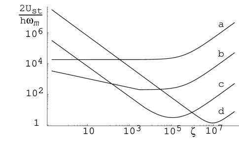
Figure 4: Rescaled steady-state energy $2U_{st}/\hbar\omega_{m}$ versus the rescaled input power $\zeta$, plotted for different values of $g_{1}$ (a: $g_{1}=10$, b: $g_{1}=10^{3}$, c: $g_{1}=10^{5}$, d: $g_{1}=10^{7}$) at fixed ${\cal Q}=10^{7}$, and with $k_{B}T/\hbar\omega_{m}=10^{5}$ and $\eta=0.8$. The optimal input power $\zeta_{opt}$ correspondingly increases, and for high gain values, ground state cooling can be achieved.

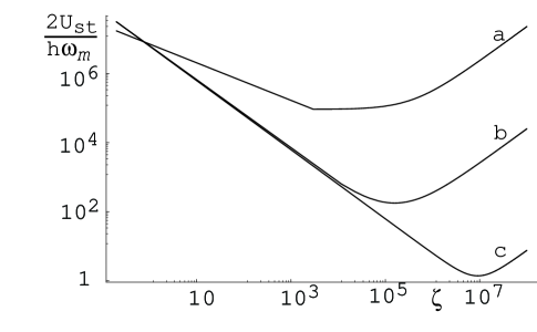
Figure 5: Rescaled steady-state energy $2U_{st}/\hbar\omega_{m}$ versus $\zeta$ for increasing values of the mechanical quality factor ${\cal Q}$ (a: ${\cal Q}=10^{3}$, b: ${\cal Q}=10^{5}$, c: ${\cal Q}=10^{7}$) at fixed $g_{1}=10^{7}$, and with $k_{B}T/\hbar\omega_{m}=10^{5}$ and $\eta=0.8$.

showing that, in the ideal limit $\eta=1$, $g_{1}\to\infty$, $\zeta\sim g_{1}\to\infty$, ${\cal Q}/g_{1}\to\infty$, also momentum feedback is able to reach the quantum limit $U_{st}=\hbar\omega_{m}/2$, i.e., it is able to cool the mirror down to its quantum ground state. The behavior of the steady-state energy is shown in Figs. 4 and 5, where $U_{st}$ (in zero-point energy units $\hbar\omega_{m}/2$) is plotted as a function of the rescaled input power $\zeta$. In Fig. 4, $2U_{st}/\hbar\omega_{m}$ is plotted for increasing values of $g_{1}$ (a: $g_{1}=10$, b: $g_{1}=10^{3}$, c: $g_{1}=10^{5}$, d: $g_{1}=10^{7}$) at fixed ${\cal Q}=10^{7}$, and with $k_{B}T/\hbar\omega_{m}=10^{5}$ and $\eta=0.8$. The figure shows the corresponding increase of the optimal input power minimizing the energy, and that for high gain values, ground state cooling can be essentially achieved, even with a nonunit detection efficiency. In Fig. 5, $2U_{st}/\hbar\omega_{m}$ is instead plotted for increasing values of the mechanical quality factor ${\cal Q}$ (a: ${\cal Q}=10^{3}$, b: ${\cal Q}=10^{5}$, c: ${\cal Q}=10^{7}$) at fixed $g_{1}=10^{7}$. The figure clearly shows the importance of ${\cal Q}$ in momentum feedback and that ground state cooling is achieved only when ${\cal Q}$ is sufficiently large. In the limit ${\cal Q}/g_{1}\to\infty$, the steady state in the presence of momentum feedback becomes very similar to that of cold damping, as it can be checked by comparing the expressions for the steady state variances in both cases. Under this limit, the two schemes have comparable cooling capabilities, even though it is evident that cold damping is more suitable to reach ground state cooling just because the requirement of a very good mechanical quality factor is not needed. The possibility to reach ground state cooling of a macroscopic mirror using the feedback scheme of Ref. MVTPRL was first pointed out, using an approximate treatment, in RON , where the need of a very large mechanical quality factor is underlined. Here we confirm this result using an exact QLE approach.

The ultimate quantum limit of ground state cooling is achieved in both schemes only if both the input power and the feedback gain go to infinity. If instead the input power is kept fixed, the effective temperature does not monotonically decrease for increasing feedback gain, but, as it can be easily seen from Eqs. (58) and (68), there is an optimal feedback gain, giving a minimum steady state energy, generally much greater than the quantum ground state energy. The existence of an optimal feedback gain at fixed input power is a consequence of the feedback-induced noise term originating from the quantum input noise of the radiation. In a classical treatment neglecting all quantum radiation noises, one would have instead erroneously concluded that the oscillator energy can be made arbitrarily small, by increasing the feedback gain, and independently of the radiation input power. This is another example of the importance of including the radiation quantum noises, showing again that a full quantum treatment is necessary to get an exhaustive description of the system dynamics LETTER .

The experimental achievement of ground state cooling via feedback is prohibitive with present day technology. For example, the experiments of Refs. HEIPRL ; PINARD ; ATTO have used feedback gains up to $g_{2}=40$ and an input power corresponding to $\zeta\simeq 1$, and it is certainly difficult to realize in practice the limit of very large gains and input powers. This is not surprising, since this would imply the preparation of a mechanical macroscopic degree of freedom in its quantum ground state, which is remarkable.

V Nonclassical effects with momentum feedback

The explicit dependence upon the mechanical quality factor ${\cal Q}$ of the steady state variances makes momentum feedback less suitable than cold damping for ground state cooling. However, the presence of an additional, in principle tunable, parameter, makes the steady state in the presence of the feedback scheme of Ref. MVTPRL richer, and capable of showing interesting and unexpected nonclassical effects at the macroscopic level.

For example, a peculiar aspect of momentum feedback is its capability of inducing steady-state correlations between the position and the momentum of the mirror, i.e., the fact that $\langle QP+PQ\rangle_{st}\neq 0$. This correlation can be evaluated solving the QLEs Eqs. (35)-(36), and one gets PRALONG

$$\frac{\langle QP+PQ\rangle_{st}}{2}=\left(\frac{\zeta}{8}+\frac{k_{B}T}{2\hbar\omega_{m}}\right)\frac{g_{1}{\cal Q}}{(1+g_{1})({\cal Q}^{2}+g_{1})}-\frac{g_{1}^{2}}{8\eta\zeta}\frac{{\cal Q}}{(1+g_{1})({\cal Q}^{2}+g_{1})}\,.$$ (70)

Due to the linearization of the problem (see Eqs. (10)-(12)), the steady state in the presence of momentum feedback is a Gaussian state, which however is never exactly a thermal state, because it is always $\langle Q^{2}\rangle_{st}\neq\langle P^{2}\rangle_{st}$ and $\langle QP+PQ\rangle_{st}\neq 0$. Its phase space contours are therefore ellipses, rotated by an angle

$$\phi=\frac{1}{2}\arctan\left[\frac{\langle QP+PQ\rangle_{st}}{\left(\langle Q^{2}\rangle_{st}-\langle P^{2}\rangle_{st}\right)}\right]$$

with respect to the $Q$ axis. The steady state becomes approximately a thermal state only in the limit of very large ${\cal Q}$ (and ${\cal Q}^{2}\gg g_{1}$), as it can be seen from Eqs. (66), (67) and (70). This thermal state approaches the quantum ground state of the oscillating mirror when also the feedback gain and the input power become very large.

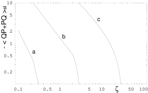
Figure 6: Steady state position-momentum correlation $-\langle QP+PQ\rangle_{st}$ versus $\zeta$ for three values of the feedback gain, $g_{1}=10^{5}$ (a), $g_{1}=10^{6}$ (b) and $g_{1}=10^{7}$ (c). The other parameters are: ${\cal Q}=10^{4}$, $k_{B}T/\hbar\omega_{m}=10^{5}$ and $\eta=0.8$.

A first example of nonclassical behavior is that this Gaussian steady state can become a contractive state, which has been shown to be able to break the standard quantum limit in YUEN , when $\langle QP+PQ\rangle_{st}$ becomes negative, and this can be achieved at sufficiently large feedback gain, that is, when $g_{1}>\eta\zeta\left(\zeta+4k_{B}T/\hbar\omega_{m}\right)$ (see Eq. (70)). This is shown in Fig. 6.

A second interesting example is that it is possible to achieve steady state position squeezing, that is, to beat the standard quantum limit $\langle Q^{2}\rangle_{st}<1/4$. The strategy is similar to that followed for cooling. First of all one has to minimize $\langle Q^{2}\rangle_{st}$ with respect to the input power $\zeta$ at fixed $g_{1}$ and ${\cal Q}$, obtaining

$$\langle Q^{2}\rangle_{st}^{min}=\frac{g_{1}{\cal Q}\sqrt{1+{\cal Q}^{2}+g_{1}}}{4\sqrt{\eta}(1+g_{1})({\cal Q}^{2}+g_{1})}+\frac{k_{B}T}{2\hbar\omega_{m}}\frac{{\cal Q}^{2}}{(1+g_{1})({\cal Q}^{2}+g_{1})}.$$ (71)

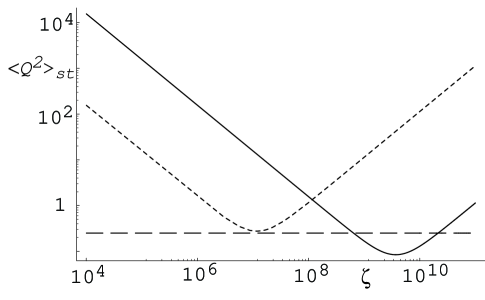
Figure 7: Steady state position variance $\langle Q^{2}\rangle_{st}$ versus $\zeta$ for two values of the feedback gain, $g_{1}=10^{7}$ (dotted line), and $g_{1}=10^{9}$ (full line). The dashed line denotes the standard quantum limit $\langle Q^{2}\rangle_{st}=1/4$, while the other parameters are: ${\cal Q}=10^{4}$, $k_{B}T/\hbar\omega_{m}=10^{5}$ and $\eta=0.8$.

This quantity can become arbitrarily small in the limit of very large feedback gain, and provided that $g_{1}\gg{\cal Q}^{2}$. That is, differently from cooling, position squeezing is achieved in the limit $g_{1}\to\infty$ (implying $\zeta\to\infty$), and there is no condition on the mechanical quality factor. Under this limiting conditions, $\langle Q^{2}\rangle_{st}$ goes to zero as $g_{1}^{-1/2}$, and, at the same time, $\langle P^{2}\rangle_{st}$ diverges as $g_{1}^{3/2}$, so that, in this limit, the steady state in the presence of momentum feedback approaches the position eigenstate with $Q=0$, that is, the mirror tends to be perfectly localized at its equilibrium position. The possibility to beat the standard quantum limit for the position uncertainty is shown in Fig. 7, where $\langle Q^{2}\rangle_{st}$ is plotted versus $\zeta$ for two different values of the feedback gain, $g_{1}=10^{7}$ (dotted line), and $g_{1}=10^{9}$ (full line), with ${\cal Q}=10^{4}$, $k_{B}T/\hbar\omega_{m}=10^{5}$, and $\eta=0.8$. For the higher value of the feedback gain, the standard quantum limit $\langle Q^{2}\rangle_{st}=1/4$ (dashed line) is beaten in a range of values of the input power $\zeta$.

This capability to achieve quantum squeezing can be exploited to get a third interesting and somewhat unexpected nonclassical effect, i.e., the possibility to have an entangled stationary state of the two movable mirrors in the ring cavity scheme of Fig. 2. This entangled state corresponds to a squeezed state of the relative motion of the two mirrors, in which their positions are strongly correlated. Such a squeezing could be obtained by applying the feedback scheme of Ref. MVTPRL to the relative motion of the mirror, which amounts to apply a continuous position shift to both mirror (see Fig. 2), in such a way that each mirror is shifted exactly opposite to the other. This means having the following additional term in the QLE for a generic operator ${\cal O}(t)$ of the two-mirror system, given by

$$\dot{{\cal O}}_{fb}(t)=i\frac{\sqrt{\gamma_{c}}}{\eta}\int_{0}^{t}dt^{\prime}G_{mf}^{-}(t^{\prime})Y_{out}(t-t^{\prime})\left[g_{mf}^{-}P_{-}(t),{\cal O}(t)\right]\,,$$ (72)

where $G_{mf}^{-}(t)$ and $g_{mf}^{-}$ are the corresponding feedback transfer function and gain factor, respectively. Assuming again a zero-delay time limit $G_{mf}^{-}(t)=\delta(t)$, the treatment of the preceding Section for a single movable mirror can be easily applied also to the case of this feedback loop acting simultaneously on the two mirrors. In fact, redefining the corresponding rescaled, dimensionless, input power of the driving laser

$$\tilde{\zeta}=\frac{32\tilde{G}^{2}\tilde{\beta}^{2}}{\gamma_{m}\gamma_{c}}=\frac{128\tilde{G}^{2}}{\hbar\omega_{0}\gamma_{m}\gamma_{c}^{2}}\wp,$$ (73)

and the corresponding rescaled feedback gain $g_{3}=-4\sqrt{2}\tilde{G}\tilde{\beta}g_{mf}^{-}/\gamma_{m}$, one gets an expression for the relative distance variance $\langle Q_{-}^{2}\rangle_{st}$ analogous to that of Eq. (66), that is,

$$\langle Q_{-}^{2}\rangle_{st}=\frac{g_{3}^{2}}{8\eta\tilde{\zeta}}\frac{1+{\cal Q}^{2}+g_{3}}{\left(1+g_{3}\right)\left({\cal Q}^{2}+g_{3}\right)}+\left[\frac{\tilde{\zeta}}{8}+\frac{k_{B}T}{2\hbar\omega_{m}}\right]\frac{{\cal Q}^{2}}{\left(1+g_{3}\right)\left({\cal Q}^{2}+g_{3}\right)},$$ (74)

Entanglement between the two mirrors in the steady state could be demonstrated using one of the sufficient critera for entanglement recently appeared in the literature TAN ; DUAN ; SIMON ; PRL02 ; REID ; NOI . The entanglement criterion easiest to satisfy is the so-called product criterion TAN ; PRL02 ; REID ; NOI , which, using the oscillator operators defined above, can be written as

$${\cal E}=16\;\langle Q_{-}^{2}\rangle_{st}\;\langle P_{+}^{2}\rangle_{st}<1\,,$$ (75)

where we have defined the marker of entanglement ${\cal E}$. This means that the two movable cavity mirrors become entangled when the above product of variances of the relative motion and of the center of mass of the system of two mirrors goes below a certain limit. The total momentum is not affected either by the radiation field, or by feedback (see Eq. (72)), and therefore it is simply given by the Brownian motion contribution $\langle P_{+}^{2}\rangle_{st}=\langle P_{+}^{2}\rangle_{BM}$, which is

$$\langle P_{+}^{2}\rangle_{BM}=\frac{k_{B}T}{2\hbar\omega_{m}}+\frac{\gamma_{m}}{\pi\omega_{m}}\ln\left(\frac{\hbar\varpi}{2\pi kT}\right).$$ (76)

In order to achieve the best conditions for entanglement one follow the same strategy adopted to get position squeezing in the Fabry-Perot cavity case, because one has essentially to squeeze the relative distance. One has first to minimize Eq. (74) with respect to the input power $\tilde{\zeta}$ at fixed $g_{3}$ and ${\cal Q}$, obtaining the optimal input power

$$\tilde{\zeta}_{opt}=\frac{g_{3}}{\cal Q}\sqrt{\frac{1+{\cal Q}^{2}+g_{3}}{\eta}}\,,$$ (77)

giving exactly expression (71) for $\langle Q_{-}^{2}\rangle_{st}^{min}$, with $g_{1}\to g_{3}$. This quantity can become arbitrarily small in the limit of very large feedback gain (implying a very large input power, see Eq. (77)) and fixed ${\cal Q}$. Since $\langle P_{+}^{2}\rangle_{st}$ does not depend upon $g_{3}$, this implies that the marker of entanglement ${\cal E}$ can be reduced below $1$. This means the possibility to entangle the two mirrors by only means of the feedback action. This is shown in Fig. 8. Notice that in such a case an extremely high feedback gain is needed, showing the difficulty in obtaining such effect. This is in apparent contrast with what has been obtained in Ref. PRL02 showing that entanglement could be achieved without feedback, and in a large temperature range, in the frequency domain, within a narrow bandwidth around the mechanical resonance. The key point is that in the present model, the feedback-induced entanglement is achieved for the full stationary state, integrated over all frequencies, and is not limited to a small bandwidth in the frequency domain. This is a much stronger effect, and it is not surprising that it is much more difficult to achieve.

VI Conclusions

We have studied how quantum feedback schemes can be used in optomechanical system to achieve cooling of vibrational degrees of freedom of a mirror. We have analysed and compared the momentum feedback scheme introduced in Ref. MVTPRL , and the cold damping scheme of HEIPRL ; PINARD ; ATTO ; COURTY . The main effect of feedback is the increase of mechanical damping, accompanied by the introduction of a controllable, measurement-induced, noise. The increase of damping means reduction of the susceptibility at resonance, and the consequent suppression of the resonance peak in the noise spectrum. We have then shown the possibility to achieve the ultimate quantum limit of ground state cooling with both feedback schemes. Cold damping is more suitable for cooling than momentum feedback because its capabilities are not influenced by the mechanical quality factor of the oscillators ${\cal Q}$. Instead momentum feedback requires a very large ${\cal Q}$, and in this limit it tends to coincide with cold damping. However, for fixed ${\cal Q}$ and for very large feedback gain (and input powers), the steady state in the presence of momentum feedback shows unexpected nonclassical features. In fact, it can become a position squeezed, or contractive state. Moreover, applying momentum feedback to the relative motion of two movable mirrors of a ring cavity, one can even get an entangled stationary state of the two mirrors, again in the limit of very large feedback gains and input powers.

Both ground state cooling and nonclassical effects are achieved in a parameter region which is extremely difficult to achieve with present day technology. This is expected, because it would imply the demonstration of genuine quantum effects for a macroscopic mechanical degree of freedom.

Figure 3: Rescaled steady-state energy $2U_{st}/\hbar\omega_{m}$ versus the rescaled input power $\zeta$, plotted for different values of $g_{2}$ (a: $g_{2}=10$, b: $g_{2}=10^{3}$, c: $g_{2}=10^{5}$, d: $g_{2}=10^{7}$), with $k_{B}T/\hbar\omega_{m}=10^{5}$ and $\eta=0.8$. The optimal input power correspondingly increases, and for high gain values, ground state cooling can be obtained.

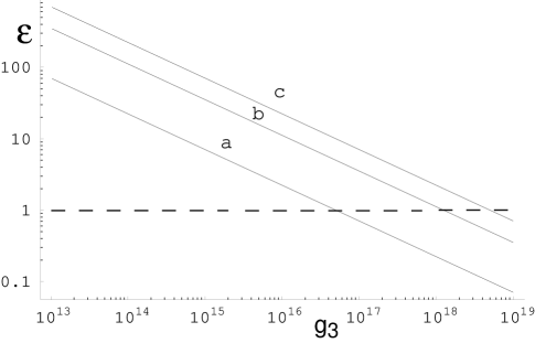
Figure 8: The marker of entanglement ${\cal E}$ is plotted versus the feedback gain $g_{1}$ for three values of the mechanical quality factor ${\cal Q}=10^{3}$ (a), ${\cal Q}=3\times 10^{3}$ (b) and ${\cal Q}=10^{4}$ (c). The other parameters are: $k_{B}T/\hbar\omega_{m}=10^{5}$ and $\eta=0.8$.

References

- (1) S. Mancini, D. Vitali, and P. Tombesi, Phys. Rev. Lett. 80, 688 (1998).
- (2) P. F. Cohadon, A. Heidmann and M. Pinard, Phys. Rev. Lett. 83, 3174 (1999).
- (3) M. Pinard, P. F. Cohadon, T. Briant and A. Heidmann, Phys. Rev. A 63, 013808 (2000).
- (4) T. Briant, P. F. Cohadon, M. Pinard, and A. Heidmann, e-print quant-ph/0207049.
- (5) S. van der Meer, Rev. Mod. Phys. 57, 689 (1985).
- (6) D. Vitali, S. Mancini, and P. Tombesi, Phys. Rev. A 64, 051401(R) (2001).
- (7) D. Vitali, S. Mancini, L. Ribichini and P. Tombesi, Phys. Rev. A 65, 063803 (2002).
- (8) M. G. Raizen, J. Koga, B. Sundaram, Y. Kishimoto, H. Takuma, and T. Tajima, Phys. Rev. A 58, 4757 (1998).
- (9) J. M. W. Milatz and J. J. van Zolingen, Physica 19, 181 (1953); J. M. W. Milatz, J. J. van Zolingen, and B. B. van Iperen, Physica 19, 195 (1953).
- (10) J-M. Courty, A. Heidmann, and M. Pinard, Eur. Phys. J. D 17, 399 (2001).
- (11) M. P. Blencowe and M. N. Wybourne, Physica B 280, 555 (2000).
- (12) A. N. Cleland and M. L. Roukes, Nature (London) 392, 160 (1998).
- (13) A. D. Armour, M. P. Blencowe, K. C. Schwab, Phys. Rev. Lett. 88, 148301 (2002).
- (14) H. M. Wiseman, Phys. Rev. A 49, 2133 (1994).
- (15) V. Giovannetti, P. Tombesi and D. Vitali, Phys. Rev. A 60, 1549 (1999).
- (16) C. M. Caves, Phys. Rev. Lett. 45, 75 (1980); R. Loudon, Phys. Rev. Lett. 47, 815 (1981); C.M. Caves, Phys. Rev. D 23, 1693 (1981); P. Samphire, R. Loudon and M. Babiker, Phys. Rev. 51, 2726 (1995).
- (17) J. Mertz, O. Marti, and J. Mlynek, Appl. Phys. Lett. 62, 2344 (1993); T. D. Stowe, K. Yasamura, T. W. Kenny, D. Botkin, K. Wago, and D. Rugar, Appl. Phys. Lett. 71, 288 (1997); G. J. Milburn, K. Jacobs, and D. F. Walls, Phys. Rev. A 50, 5256 (1994).
- (18) M. Pinard, Y. Hadjar, and A. Heidmann, Eur. Phys. J. D 7, 107 (1999).
- (19) C. K. Law, Phys. Rev. A 51, 2537 (1995).
- (20) A. F. Pace, M. J. Collett, and D. F. Walls, Phys. Rev. A 47, 3173 (1993); K. Jacobs, P. Tombesi, M. J. Collett, and D. F. Walls, Phys. Rev. A 49, 1961 (1994); S. Mancini and P. Tombesi, Phys. Rev. A 49, 4055 (1994).
- (21) K. Jacobs, I. Tittonen, H. M. Wiseman, and S. Schiller, Phys. Rev. A 60, 538 (1999).
- (22) Y. Hadjar, P. F. Cohadon, C. G. Aminoff, M. Pinard, and A. Heidmann, Europhys. Lett. 47, 545 (1999).
- (23) I. Tittonen, G. Breitenbach, T. Kalkbrenner, T. Müller, R. Conradt, S. Schiller, E. Steinsland, N. Blanc, and N. F. de Rooij, Phys. Rev. A 59, 1038 (1999).
- (24) C. W. Gardiner, Quantum Noise (Springer-Verlag, Berlin, 1991).
- (25) V. Giovannetti and D. Vitali, Phys. Rev. A 63 023812 (2001).
- (26) H. Grabert, U. Weiss, P. Talkner, Z. Phys. B 55, 87 (1984).
- (27) F. Haake and R. Reibold, Phys. Rev. A 32, 2462 (1985).
- (28) H. M. Wiseman, and G.J. Milburn, Phys. Rev. A 47, 642 (1993).
- (29) F. Grassia, J. M. Courty, S. Reynaud and P. Touboul, Eur. Phys. J. D 8, 101 (2000).
- (30) R. Folman, J. Schmiedmayer, H. Ritsch, and D. Vitali, Eur. Phys. J. D, 13, 93 (2001).
- (31) H. P. Yuen, Phys. Rev. Lett. 51, 719 (1983); M. Ozawa, Phys. Rev. Lett. 60, 385 (1988).
- (32) S. M. Tan, Phys. Rev. A 60, 2752 (1999).
- (33) L. M. Duan, et al., Phys. Rev. Lett. 84, 2722 (2000);
- (34) R. Simon, Phys. Rev. Lett. 84, 2726 (2000).
- (35) S. Mancini, V. Giovannetti, D. Vitali and P. Tombesi, Phys. Rev. Lett. 88, 120401 (2002).
- (36) M. D. Reid, e-print quant-ph/0112038.
- (37) S. Mancini, D. Vitali, V. Giovannetti, and P. Tombesi, quant-ph/0209014.