Laser cooling of trapped Fermi gases

Abstract

The collective Raman cooling of trapped one- and two-component Fermi gases is considered. We obtain the quantum master equation that describes the laser cooling in the festina lente regime, for which the heating due to photon reabsorption can be neglected. For the two-component case the collisional processes are described within the formalism of quantum Boltzmann master equation. The inhibition of the spontaneous emission can be overcome by properly adjusting the spontaneous Raman rate during the cooling. Our numerical results based in Monte Carlo simulations of the corresponding rate equations, show that three-dimensional temperatures of the order of $0.08$ $T_{F}$ (single-component) and $0.03$ $T_{F}$ (two-component) can be achieved. We investigate the statistical properties of the equilibrium distribution of the laser-cooled gas, showing that the number fluctuations are enhanced compared with the thermal distribution close to the Fermi surface. Finally, we analyze the heating related to the background losses, concluding that our laser-cooling scheme should maintain the temperature of the gas without significant additional losses.

I Introduction

The achievement of Bose-Einstein condensation (BEC) BEC in trapped dilute atomic gases has stimulated a large interest in the physics of ultracold gases, both bosonic and fermionic ones. Related with the latter, similar cooling methods as those employed to reach BEC have been recently employed to accomplish a degenerate Fermi gas, i.e. a Fermi gas with temperature $T$ below the Fermi temperature ($T_{F}$) Jin ; Schreck ; Hulet ; Granade ; Hadzibabic ; Roati . For $T<T_{F}$ the Fermi pressure becomes noticeable, and as a consequence the Fermi cloud becomes significantly broader than a BEC under the same temperature. Additionally, for temperatures below a critical one, $T_{c}$, the system should undergo a Bardeen-Cooper-Schrieffer (BCS) transition DeGennes . When this occurs the system becomes superfluid, due to the Cooper pairing of particles near the Fermi surface. The accomplishment of BCS pairing and its observation have been considered in detail Stoof ; Baranov ; Houbiers ; Bruun . However, the employed cooling schemes have not yet allowed for temperatures below $T_{c}$, which has been predicted to be much smaller than $T_{F}$. Those cooling methods rely on collisional processes, which in the degenerate regime are strongly suppressed due to Pauli blocking. As a consequence, the cooling efficiency decreases, and technical losses have prevented until now from reaching temperatures well below $T_{F}$ HollandF . Recently, however, it has been proposed that the latter obstacle could be overcome by employing Feshbach resonances Holland ; Griffin or optical lattices OptLatt in order to increase the ratio $T_{c}/T_{F}$ up to $\approx 0.2$, opening the possibility to achieve BCS in a temperature range where the collisional processes are still efficient enough. In fact, very recently temperatures $T\leq 0.2T_{F}$ have been reported by O’Hara et al. OHara , which are below the predicted value of $T_{C}$.

In this paper we show that laser cooling could provide an effective and realistic tool to cool one- and two-component Fermi gases well below $T_{F}$. The proposed method is realized in the festina lente (FL) regime Festina , in which the spontaneous emission rate $\gamma$ is smaller than the trap frequency $\omega$. In this regime the heating introduced by photon reabsorptions can be suppressed. In the absence of technical losses the major limitation to the laser cooling in the festina lente regime is set up by the finite value of Lamb-Dicke parameter, defined as the square root of the ratio of the recoil energy to $\hbar\omega$. In practice, when the spontaneous emission rate becomes much smaller than the trap frequency, the finite available time sets limit on achievable temperatures, due to always present loss mechanism. Reaching FL regime is experimentally feasible, and has been in fact demonstrated in experiments by the group of Weiss Weiss ; Salomon , in which a suppression of reabsorptions for decreasing $\gamma/\omega$ has been observed for tightly bound atoms in an optical lattice. The laser cooling in the FL regime down to the quantum degeneracy has been already predicted to work for bosons 1atom ; Natoms and for polarized fermions fermicool . The latter case is particularly interesting, since evaporative cooling cannot be employed to a single-component fermionic system, due to the absence of $s$-wave scattering, while less restrictive, sympathetic cooling techniques Schreck ; Hulet ; Hadzibabic ; Roati , are also eventually limited due to Pauli blocking. The BCS transition in such a system could be realized by externally inducing interatomic interactions, for instance dipole-dipole ones dipols .

In the present paper we analyze the three-dimensional laser cooling of Fermi gases down to temperatures $T\ll T_{F}$, by performing Monte Carlo simulations of the quantum dynamics governed by the Master Equation (ME). For $T$ comparable to $T_{F}$, the laser cooling of fermions is affected by the statistical inhibition of the spontaneous emission, which results in a decrease of the cooling efficiency. In a previous work fermicool we have analyzed the laser cooling of a polarized Fermi gas. We have theoretically predicted that the above mentioned problem can be overcome by either dynamically adjusting the spontaneous emission rate in a Raman cooling process, or by employing appropriately designed anharmonic traps.

We first consider the single-component case. In particular, we analyze the statistics of the laser-cooled gases, comparing the results with those expected for a thermal distribution. We show that whereas the mean-number distribution can be well approximated by a corresponding thermal one, the fluctuations significantly differ from the thermal case. This could have significant effects in the BCS pairing of these gases after an interatomic interaction is induced in the way discussed above.

In the second part of this work, we analyze the laser-cooling of a two-component Fermi gas. For this case, the collisions between different components cannot be neglected. We consider them within the formalism of Quantum Boltzmann Master Equation (QBME). This formalism is shown to produced the expected thermal distribution in the absence of laser cooling. We analyze the case in which only one of the fermionic species is laser-cooled, whereas the other one is sympathetically cooled as a result of the collisions between different components. We show that the laser-cooling is significantly favored by the presence of the second component. We analyzed also the statistics of the atom distribution, showing that the fluctuations at the Fermi surface are significantly enhanced compared to the thermal case. Finally, we analyze the heating induced by background collisions, and show that the laser cooling can be employed to maintain a two-component Fermi gas at a fixed temperature for a relatively long time without significant atom losses.

The paper is organized as follows. In section II, we discuss our cooling scheme, and obtain the ME that describes the Raman cooling in the FL regime. We also describe in this section the corresponding ME for the two-component case. We present the resulting rate equations and discuss their physical properties. In section III we present our numerical results concerning the laser cooling of a single component gas, characterizing the statistical properties of the laser-cooled gas. In section IV we present our results for the case of a two–component Fermi gas, in which one of the components is laser-cooled. We discuss the statistics for this case, as well as the heating induced by losses, and its control using laser-cooling. We finalize in section V with some conclusions.

II Quantum Master Equation

We consider $N$ fermionic atoms with an accessible electronic three–level $\Lambda$ scheme, with levels $|g\rangle$, $|e\rangle$ and $|r\rangle$. We assume that the ground state $|g\rangle$ is coupled via a Raman transition to $|e\rangle$ (which is assumed metastable). Another laser couples $|e\rangle$ to the upper state $|r\rangle$, which rapidly decays into $|g\rangle$. After the adiabatic elimination of $|r\rangle$, a two–level system is obtained, with an effective Rabi frequency $\Omega$, and an effective spontaneous emission rate $\gamma$. The latter can be controlled by modifying the coupling from $|e\rangle$ to $|r\rangle$. The atoms are confined in a non-isotropic dipole trap with frequencies $\omega^{g}_{x,y,z}$, $\omega^{e}_{x,y,z}$, different for the ground and the excited states, and non-commensurable one with another. The latter assumption simplifies enormously the dynamics of the spontaneous emission processes in the FL limit. When deriving the quantum ME, it is important to cancel the off-diagonal terms of the density matrix, in order to reduce the ME to a rate equation, which is possible to simulate numerically with Monte Carlo methods. The anisotropy of the trap does not need to be very large, and for practical purposes can be rather small. Its effects in the rate equations is not relevant at all, and consequently in our simulation we consider the simple case of isotropic trap. The cooling process consists of sequences of Raman pulses of appropriate frequencies, adjusted is such a way that they induce the transition of atoms to the lower motional states of the trap. We assume weak optical excitation, so that no significant population in $|e\rangle$ is present. This allows to adiabatically eliminate $|e\rangle$, and consequently to consider only the density matrix $\rho(t)$ describing all atoms in $|g\rangle$, and being diagonal in the Fock representation corresponding to the bare trap levels.

Let us introduce the annihilation and creation operators of atoms in the ground (excited) state and in the trap level $m$ ($l$), which we denote by $g_{m}$, $g_{m}^{{\dagger}}$ ($e_{l}$, $e_{l}^{{\dagger}}$). These operators fulfill standard fermionic anticommutation relations: $\{g_{m},g_{n}^{{\dagger}}\}=\delta_{m,n}$, $\{e_{m},e_{n}^{{\dagger}}\}=\delta_{m,n}$. We use the standard theory of quantum-stochastic processes GardinerB ; Carmichael to develop the quantum ME that governs the dynamics of cooling Castin . The derivation of the ME for fermions proceeds basically in a similar way to the corresponding derivation for bosons. The latter was presented in details in Natoms . The ME that describes the dynamics of the density matrix $\rho$ of the atoms in the FL regime is

$$\dot{\rho}(t)={\cal L}_{0}\rho+{\cal L}_{1}\rho,$$ (1)

where

$${\cal L}_{0}\rho = -i\hat{H}_{eff}\rho(t)+i\rho(t)\hat{H}_{eff}^{{\dagger}}+{\cal J}\rho(t),$$ (2)

$${\cal L}_{1}\rho = -i[\hat{H}_{las},\rho(t)],$$ (3)

with

$$\hat{H}_{eff} = \sum_{m}\omega_{m}^{g}g_{m}^{{\dagger}}g_{m}+\sum_{l}(\omega_{l}^{e}-\delta)e_{l}^{{\dagger}}e_{l}$$ (4)

$$- i\gamma\sum_{l,m}\xi_{lm}e_{l}^{{\dagger}}g_{m}g_{m}^{{\dagger}}e_{l},$$

$$\hat{H}_{las} = \frac{\Omega}{2}\sum_{l,m}\eta_{lm}(k_{L})e_{l}^{{\dagger}}g_{m}+H.c.,$$ (5)

$${\cal J}\rho(t) = 2\gamma\sum_{l,m}\xi_{lm}g_{m}^{{\dagger}}e_{l}\rho(t)e_{l}^{{\dagger}}g_{m}.$$ (6)

Here, $2\gamma$ is the single–atom effective spontaneous emission rate, $\Omega$ is the Rabi frequency associated with the atom transition and the laser field, $\omega_{m}^{g}$ ($\omega_{l}^{e}$) are the energies of the ground (excited) harmonic trap level $m$ ($l$), $\delta$ is the laser detuning from the atomic transition, $\xi_{lm}=\int_{0}^{2\pi}d\phi\int_{0}^{\pi}d\theta\,\sin\theta\,{\cal W}(\theta,\phi)|\eta_{lm}(\vec{k})|^{2}$, where ${\cal W}(\theta,\phi)$ is the fluorescence dipole pattern, and $\eta_{lm}(k_{L})=\langle e,l|e^{i\vec{k}_{L}\cdot\vec{r}}|g,m\rangle$ are the Frank–Condon factors. In the following we assume that $\Omega<\gamma$ and $\Omega^{2}/\gamma\ll\omega$, which allows for adiabatic elimination of excited state $|e\rangle$. To assure the FL regime we require also $\gamma<\omega$ at least in the initial phase of the cooling process.

The dynamics of the two-component system in the FL limit, where only the first component is laser cooled, may be described by the following ME:

$$\dot{\rho}(t)={\cal L}_{0}\rho+{\cal L}_{1}\rho+{\cal L}_{2}\rho.$$ (7)

The new term ${\cal L}_{2}$ that appears in Equation (7) describes the process of elastic collisions between the two species:

$${\cal L}_{2}\rho = -i[\hat{H}_{coll},\rho(t)],$$ (8)

where

$$\hat{H}_{coll}=\sum_{n,m,q,p}U_{n,m;q,p}g_{n}^{{\dagger}}b_{m}^{{\dagger}}b_{q}g_{p}.$$ (9)

Here, $b_{m}$ and $b_{m}^{{\dagger}}$ are respectively the annihilation and creation operators of atoms of the second component in the trap state $m$. Since at low temperatures collisions between atoms are purely of $s$-wave type, the operator $\hat{H}_{coll}$ accounts only for collisions between atoms in the second component and those atoms in the ground electronic state $|g\rangle$ of the first species. The collisions with the atoms in the $|e\rangle$ can be neglected if the laser is sufficiently weak to assure that only a small fraction of atoms is excited in each pulse. The amplitude $U_{n,m;p,q}$ in Equation (9) reads

$$U_{n,m;q,p}=\frac{4\pi\hbar a_{sc}}{m}\int_{R^{3}}d^{3}x\phi_{n}^{\ast}({\bf x})\beta_{m}^{\ast}({\bf x})\beta_{q}({\bf x})\phi_{p}({\bf x}),$$ (10)

where $\phi_{n}$ ($\beta_{n}$) denotes the wavefunction of the $n$-th level of the $|g\rangle$, ($|b\rangle$) trap, and $a_{sc}$ is the scattering length. The term ${\cal L}_{1}$ from the ME (7), includes the effective Hamiltonian $H_{eff}$, which in the presence of two components, accounts also for the energies of atoms of the second component

$$\hat{H}_{eff} = \sum_{m}\omega_{m}^{g}g_{m}^{{\dagger}}g_{m}+\sum_{l}(\omega_{l}^{e}-\delta)e_{l}^{{\dagger}}e_{l}+$$ (11)

$$+ \sum_{n}\omega_{n}^{b}b_{n}^{{\dagger}}b_{n}-i\gamma\sum_{l,m}\xi_{lm}e_{l}^{{\dagger}}g_{m}g_{m}^{{\dagger}}e_{l}.$$

For the assumed regime of parameters, the excited state may be adiabatically eliminated. To this end we use standard projection operator techniques GardinerB . The corresponding calculus proceed in the same way as in the case of bosons, which was described in detail in Natoms . Here, we present only the final results. For sufficiently weak interactions between the two species, the dynamics due to the collisions and the dynamics due to the laser–cooling are independent Coll . The process of laser cooling may be described by the ME (1) without the collisional part, while the collisional part of dynamics after the adiabatic elimination takes the form of QBME, similar to the one formulated for bosons and presented in Gardiner1 ; Gardiner2 . The rate equations for the populations $N_{n}^{1}$ and $N_{m}^{2}$ in level $n$ and $m$ of the trap $|g\rangle$ and $|b\rangle$ respectively, are given by

$$\dot{N}_{n}^{1} = \sum_{p}P^{opt}_{p\rightarrow n}N_{p}^{1}+\sum_{m,p,q}P^{coll}_{p,q\rightarrow n,m}N_{p}^{1}N_{q}^{2}$$ (12)

$$\mbox{}-\sum_{p}P^{opt}_{n\rightarrow p}N_{n}^{1}-\sum_{m,p,q}P^{coll}_{n,m\rightarrow p,q}N_{n}^{1}N_{m}^{2},$$

$$\dot{N}_{m}^{2} = \sum_{n,p,q}P^{coll}_{p,q\rightarrow n,m}N_{p}^{1}N_{q}^{2}$$ (13)

$$\mbox{}-\sum_{n,p,q}P^{coll}_{n,m\rightarrow p,q}N_{n}^{1}N_{m}^{2},$$

where $P^{opt}_{p\rightarrow n}$ is the rate of laser-induced transition from state $m$ to state $n$ of the $|g\rangle$ trap

$$P^{opt}_{p\rightarrow n} = \frac{\Omega^{2}}{2\gamma}(1-N_{n}^{1})\times$$

$$\times \sum_{l} \frac{\gamma^{2}\xi_{ln}\eta_{lp}(k_{L})}{[\delta-(\omega_{l}^{e}-\omega_{p}^{g})]^{2}+\gamma^{2}(R_{l}+\xi_{lp})^{2}},$$ (14)

with $R_{l}=\sum_{n^{\prime}}\xi_{ln^{\prime}}(1-N_{n^{\prime}}^{1})$. The rate $P^{coll}_{p,q\rightarrow n,m}$ of a collision between two fermions of different species, occupying the states $p$ and $q$ of the trap respectively, resulting in a transition to the states $n$ and $m$, is given by

$$P^{coll}_{p,q\rightarrow n,m}=\frac{\pi}{\omega}\left|U_{n,m;q,p}\right|^{2}\delta_{E_{n}+E_{m},E_{p}+E_{q}}(1-N_{n}^{1})(1-N_{m}^{2}).$$ (15)

In the transition rate (14) one can clearly identify two contributions due to the quantum–statistical character of fermions: (a) If the system becomes more degenerate, $R_{l}$ vanishes, and the atoms remain for very long times in the excited state $l$, i.e. the spontaneous emission is inhibited. This affects negatively the cooling process in two ways: first, it prolongs the cooling, and second, the excited-ground collisions can occur and lead to heating and losses. In addition, the adiabatic elimination used in the derivation of Equation. (14) ceases to be valid. (b) The fermionic inhibition factor $(1-N_{n})$ appears in the numerator of the probabilities, introducing also a slowing-down of the cooling process.

The negative influence of Fermi statistics above can be overcome by dynamically changing of $\gamma$ in Raman cooling fermicool . One can increase it gradually during the cooling in order to avoid the inhibition effects, but still remaining in the FL regime. Note that, the FL condition involves the spontaneous emission rate modified in the presence of other atoms: $\gamma R_{l}<\omega$. Still, even if one uses such approach some small fraction of the atoms will remain in the excited state after the cooling pulse, and has to be removed from the trap in order to avoid non-elastic collisions. The latter aim can be achieved by optically pumping the excited atoms to a third non-trapped level. This introduces a new loss mechanism which we take into account in the simulations.

The calculations of the laser cooling were performed for the case of a three-dimensional harmonic trap. For simplicity we assumed that the trap is isotropic with frequency $\omega$. The main difficulty for performing Monte–Carlo simulations of the laser–cooling for fermions is the large number of states in the calculation. Since one state can be populated maximally by one fermion, in order to perform a simulation for a medium-size atomic sample (in our case $10^{4}$ atoms), we had to consider rather large trap ( $80$ energy levels in our case). In addition if the simulation starts from a temperature above $T_{F}$, the number of states must be much larger than the number of atoms in the trap. For an initial number of $10^{4}$ atoms, we calculated the cooling dynamics for the trap consisting of approximately $10^{5}$ states. For a single component gas of fermions, where the collisions between the atoms are absent, we were able to perform simulations treating each state of the trap separately. In this case the transition is only induced by the laser, and its rate given by (14) depends only on two states. The number of different probabilities that one have to recalculate after the change of the atomic distribution is roughly $10^{9}$.

In the case of the two–component Fermi gas, one has to account for the process of collisions, in which the transition rate (15) depends on four numbers: two initial states and two final states. The number of different probabilities that one has to recalculate after a single transition takes place is roughly $10^{18}$. The number of operations required to calculate the probabilities is orders of magnitude too large for numerical computations. Therefore for simulating the cooling in two-species gas, we have applied the ergodic approximation. We assume that the populations of the states with the same energy are equal: $N_{m}^{n}=\bar{N}_{E(m)}^{n}/g_{E(m)}$, where $n\in\{1,2\}$, $\bar{N}_{E}^{n}$ is the number of atoms of the $n$-th component occupying the energy shell $E$ and $g_{E}$ is the degeneracy of the energy shell $E$. This approximation relies on the fact that for typical parameters, the collisional processes are much faster than the laser cooling. Additionally the thermalization inside a single energy shell is much faster than the thermalization between energy shells of different energies.

The assumption that collisions occur much more frequently than laser induced transitions, is necessary, since the laser cooling is not fully “compatible” with the ergodic approximation. The cooling is based on the process of absorption of a photon from one of three orthogonal laser beams, therefore the rate of transition depends on the three dimensional structure of the initial and the final state. Due to this dependence, we have not been able to find a simpler formula, which would be a counterpart of Equation (14) in ergodic approximation. In the case of the collisional process, however, one can further develop the rate (15) in order to fully utilize the advantages of the ergodic approximation.

The rate of collision, between fermions occupying the energy shells $e_{1}$ and $e_{2}$, resulting in a transition to the energy shells $e_{3}$ and $e_{4}$ in the ergodic approximation is given by

$$P^{coll}_{e_{1},e_{2}\rightarrow e_{3},e_{4}}=\frac{\pi}{\omega}\frac{(g_{e_{3}}-\bar{N}_{e_{3}}^{1})(g_{e_{4}}-\bar{N}_{e_{4}}^{2})}{g_{e_{1}}g_{e_{2}}g_{e_{3}}g_{e_{4}}}\left|\tilde{U}_{e_{1},e_{2};e_{3},e_{4}}\right|^{2},$$ (16)

where the amplitude of the transition $\tilde{U}_{e_{1},e_{2};e_{3},e_{4}}$ is defined as follows

$$\left|\tilde{U}_{e_{1},e_{2};e_{3},e_{4}}\right|^{2} = \sum_{n,m,p,q}\delta_{E_{p},e_{1}}\delta_{E_{q},e_{2}}\delta_{E_{n},e_{3}}\delta_{E_{m},e_{4}}\times$$ (17)

$$\times \left|U_{n,m;q,p}\right|^{2}.$$

In principle, the amplitude of transition $\tilde{U}_{e_{1},e_{2};e_{3},e_{4}}$ may be calculated directly from Equation. (17), by performing a summation of the terms $\left|U_{n,m;q,p}\right|^{2}$ given by formula (10). This requires, however, a lot of numerical efforts, since the number of operations is of the order $N_{st}^{4}$, where $N_{st}$ is the number of states in the trap. This can be avoided, if the trap is isotropic, in which case we were able to derive a simplified expression

$$\left|\tilde{U}_{e_{1},e_{2};e_{3},e_{4}}\right|^{2} = \frac{2}{\pi^{4}}\left(\frac{4\pi\hbar a_{sc}}{m\xi^{3}}\right)^{2}\times$$ (18)

$$\times \sum_{n,m,p,q}\frac{I_{nmpq}^{4}I_{nmpq}^{0}-(I_{nmpq}^{2})^{2}}{2^{n+m+p+q}n!m!p!q!},$$

where $\xi=\sqrt{\hbar/m\omega}$. The coefficients $I_{nmpq}^{k}$ are defined by

$$I_{nmpq}^{k}=\int_{-\infty}^{\infty}dxe^{-x^{2}}x^{k}H_{n}(x)H_{m}(x)H_{p}(x)H_{q}(x),$$ (19)

where $H_{n}(x)$ denotes the $n$-th Hermite polynomial. Note that the summation over indices $n$ ($m$, $p$, $q$) in Equation (18), runs from $0$ if $e_{n}$ ($e_{m}$, $e_{p}$, $e_{q}$) is even, or from $1$ if $e_{n}$ ($e_{m}$, $e_{p}$, $e_{q}$) is odd, up to $e_{n}$ ($e_{m}$, $e_{p}$, $e_{q}$) with an increment equal to $2$. In order to obtain Equation (18), we have used standard summation formulas for Hermite polynomials Ryzhik . Equation (18) can be further simplified, if the collisions involves distant energy shells, i.e. the minimum $e_{min}$ of the set of numbers $\{e_{1},e_{2};e_{3},e_{4}\}$ is much smaller than its maximum $e_{max}$. According to Ref. HollandB , the following approximate formula holds

$$\left|\tilde{U}_{e_{1},e_{2};e_{3},e_{4}}\right|^{2}\simeq\left(\frac{4\pi\hbar a_{sc}}{m\xi^{3}}\right)^{2}\frac{g_{e_{min}}}{4\pi^{4}}.$$ (20)

With the help of the exact expression (18), we have verified numerically that the approximation (20) gives correct results, already for $e_{max}-e_{min}\gtrsim 2\hbar\omega$. Equation (20) leads to small errors for low lying energy shells, and for the transitions between neighboring shells. In the simulations, however, we have used the values calculated numerically with the help of the exact formula (18).

III Results for one–component gas

The numerical simulations of the cooling were performed using Monte Carlo techniques. In the calculation we assumed that the atoms are confined in a dipole trap, characterized by a Lamb-Dicke parameter $\eta=2\pi a/\lambda=2$, with $a=\sqrt{\hbar/2m\omega}$ being the size of the ground state of the trap, and $\lambda$ the laser wavelength. In the context of laser cooling, an optical dipole trap was recently employed in experiments on all-optical production of a degenerate gas of two species of Li Granade , and it is also considered in current experiments in Mg Ernst . Due to numerical limitations we assumed Lamb-Dicke parameter $\eta=2$ LambDicke . The assumed value of $\eta$ is not unrealistic, and can be realized for instance by trapping potassium atoms in a dipole trap with $\omega=2\pi\times 2.4$ kHz, which is the trapping frequency employed in experiments in $Li$ Granade , and a laser wavelength $\lambda\simeq 720$ nm. In the calculation we use the above mentioned values to calculate real cooling time. We start our simulations with an initial number of atoms $N=10660$, which corresponds to a Fermi energy $E_{F}=38\hbar\omega$. The three-dimensional isotropic harmonic trap contains $81$ energy levels, which corresponds to $91881$ states.

In the gas of fermions the main sources of losses are background collisions and photoassociation. Background collisions result from non ideal vacuum conditions in the experiment, and introduce a relevant heating mechanism for temperatures well below Fermi temperature Timmer . In the simulations we assumed a background collision rate $\gamma_{bg}=1/350$ Hz HollandF . Photoassociation losses (when the laser is tuned between molecular resonances) are typically of the order of $10^{-14}$cm³/s for laser intensities of $1$mW/cm² Machholm . In our case the laser intensities needed are typically $1000$ times smaller and we estimate that for $N=10660$ atoms, the atomic density is smaller than $3.5\times 10^{14}$cm^-3. Therefore the photoassociation losses can be safely neglected. The other type of losses which we account for in our calculations is the removal process of long-living excited atoms at the end of each cooling pulse.

Figure 1 shows the time-dependence of the temperature of a laser-cooled one-component gas of fermions. The inset shows the time dependence of the number of fermions, that decreases due to losses. As the initial state of the system we consider a thermal distribution with temperature $T_{0}=1.04T_{F}$. The cooling process was divided into three stages, each consisting of a sequence of two Raman pulses. The employed pulses that are used are characterized by the following parameters: detuning $\delta/\omega=\{(-11,-12)$, $(-16,-17)$, $(-19,-20)\}$ respectively, Rabi frequency $\Omega/\gamma=\{(0.013,0.013)$, $(0.007,0.01)$, $(0.1,0.8)\}$ respectively, and length $\Delta t/\omega^{-1}=\{(250,250)$, $(500,500)$, $(2000,4000)\}$ respectively. The use of two pulses with slightly different detunings in each cooling stage allows to compensate for the oscillatory character of the Frank-Condon factors. The values of $\Omega$ were chosen in such way that not more than $10\%$ of the atoms is excited during each pulse, in order to fulfill the condition of the adiabatic elimination. The temperature of the system was determined by fitting of the thermal distribution to the current distribution of fermions. At the end of cooling, the system reaches the temperature $T=0.08T_{F}$.

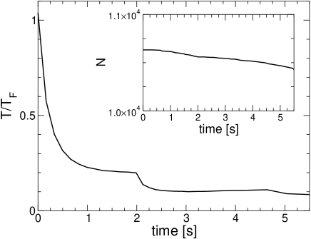
Figure 1: Time-dependence of the temperature during the laser cooling of a single component Fermi gas by controlling the effective spontaneous Raman rate. Inset: time dependence of the number of atoms, which decreases due to background collisions and the removal of long-living excited atoms. The different Raman cooling stages discussed in the text extend from $0$ $s$ to $2$ $s$, from $2$ $s$ to $4.6$ $s$, and from $4.6$ $s$ to $5.5$ $s$.

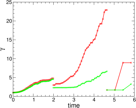
Figure 2: Time-dependence of the effective single-atom spontaneous emission rate for the case considered in Fig. 1. The values for the first pulse in the sequence (solid line with diamonds) and those for the second pulse (solid line with squares) are indicated. The different Raman cooling stages discussed in the text extend from $0$ $s$ to $2$ $s$, from $2$ $s$ to $4.6$ $s$, and from $4.6$ $s$ to $5.5$ $s$.

The time dependence of the spontaneous emission rate is presented in Figure 2. The two curves depict the values for the two pulses used at each stage of cooling. From this figure one can see how $\gamma$ was controlled in order to speed up the cooling, and at the same time avoid inhibition of the spontaneous emission, and remain in the festina lente regime. In the simulation it was realized by increasing of $\gamma$ gradually during the cooling process, in such a way that the average value of the spontaneous emission rate calculated for many-atom system: $\gamma_{N}$, remains approximately constant, and equal to $0.8\omega$, except for the last pulses. In the last cooling stage rather long pulses were applied, and therefore $\gamma_{N}$ could be considered smaller than in the other pulses. The expectation value of $\gamma_{N}$ is presented on Figure 3. It was calculated at the end of each pulse, averaging over all possible laser-induced transition that may take place. With each transition $m\rightarrow n$ one can associate the spontaneous emission rate $\gamma_{N}(l)=\gamma R_{l}$, where $l$ denote an intermediate state, when the atom is excited.

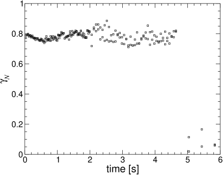
Figure 3: Time-dependence of the expectation value of the spontaneous emission rate for the case considered in Fig. 1. The spontaneous emission rate $\gamma_{N}$ takes into account the inhibition due to the presence of the other fermions in the trap. The average was calculated for the atomic distribution after each cooling pulse. The different Raman cooling stages discussed in the text extend from $0$ $s$ to $2$ $s$, from $2$ $s$ to $4.6$ $s$, and from $4.6$ $s$ to $5.5$ $s$.

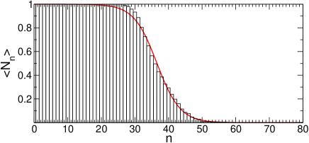
Figure 4: Mean distribution of fermions (bars) obtained by averaging in time during the prolonged last stage of the cooling process presented in Fig. 1. Solid line - fit of the thermal distribution.

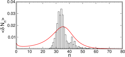
Figure 5: Fluctuations of the distribution of fermions (bars) obtained by averaging in time during the prolonged last stage of the cooling process presented in Fig. 1. Solid line - fluctuations of the thermal gas, with the temperature and the chemical potential determined from the fit of the mean distribution.

At the end of the cooling process, the temperature of the gas of fermions stabilizes and the system reaches an equilibrium distribution. In the absence of collisions, this distribution is purely determined by the laser–induced transitions, and in general may be very different than the thermal distribution. In order to investigate this point, we studied the mean population and the fluctuations of the energy shells. The statistics was calculated by time-averaging during the last stage of cooling. To this end, the final stage of cooling was extended to the time $t=4\times 10^{5}\omega^{-1}\approx 26s$. This time correspond, in average to four absorption and spontaneous emission cycles for each atom. The average distribution of atoms is plotted in Figure 4. The bars depict the distribution obtained from the simulation, whereas the solid line shows the fit of the thermal distribution. According to Figure 4, the mean population numbers are well described in the framework of the grand canonical ensemble. The fluctuations of the occupation numbers are presented in Figure 5. The solid line as before represents the fluctuations of the thermal gas, with the temperature and the chemical potential determined from the fit of the mean distribution. As can be seen, the fluctuations in the laser cooled gas have completely different properties than the fluctuations in the thermal distribution. In a small energy range below $E_{F}$, the fluctuations are enhanced, whereas deeply in the Fermi sea they completely vanish. From this peculiar behavior we may conclude that the laser cooling strongly affects the atoms near the Fermi surface. On the other hand, it does not excite those atoms deeply in the Fermi sea, due to the large negative detunings of the employed pulses.

The existence of such non-thermal fluctuations is a peculiar feature of the proposed cooling method. The observed enhancement of the fluctuation near the Fermi energy could have an important influence on the formation of Cooper pairs in laser cooled Fermi gases. This question, however, lies beyond the scope of this paper and it will be the subject of further investigations. It is worth stressing that our cooling scheme can be applied to a Fermi mixture with scattering length modified in the vicinity of a Feshbach resonance. With the help of this technique, the critical temperature for the BCS transition is predicted to reach $0.2$-$0.5$ $T_{F}$ Holland ; Griffin . Laser cooling should then allow to achieve such temperatures, presumably in a time scale shorter that $1$ $s$ (see Figure 1).

IV Results for two–component gas

In the simulation of laser cooling in the two–component Fermi system we considered the same parameters as in the case of the single component gas. We assumed that the two species are placed in the same isotropic optical trap with frequency $\omega=2\pi\times 2.4$ kHz. The Lamb-Dicke parameter is $\eta=2$ and the wavelength of the cooling laser is $\lambda\simeq 720$ nm. The trap considered in the simulation has the same depth for both species, and contains $81$ energy levels. The losses due to the background collisions affect in this case both components. In the simulations we assumed the same background-collision rate $\gamma_{bg}=1/350$ Hz for both species. The two components have equal initial number of atoms $N=10660$. The scattering length for the interactions between the two species is equal to $a_{sc}=157a_{0}$, where $a_{0}$ is the Bohr radius. This value correspond to the interactions between two spin states $|F=9/2,m_{F}=9/2\rangle$ and $|F=9/2,m_{F}=7/2\rangle$ of ⁴⁰K DeMarco .

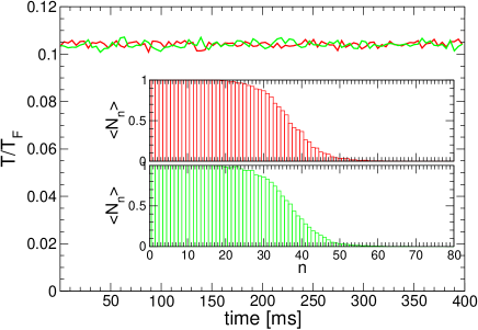
Figure 6: Time dependence of the temperatures of the two components during the evolution in the presence of collisions only. The inset presents the final distribution of the first component (upper plot) and of the second component (lower plot).

Our first aim was to investigate the dynamics and the properties of the equilibrium distribution of the two–component Fermi gas where the collisions are described by the QBME, and the resulting probabilities (15). In this case we do not take into account the laser cooling mechanism. The energy levels in the trap are initially populated according to a thermal distribution with temperature $T=0.1T_{F}$. Then, we let the system evolve in the presence of collisions during a time $t=400$ ms, corresponding to about $30$ collisions per atom in average. The time dependence of the temperatures of the two components is presented in Figure 6, whereas the inset shows their final distributions. As one can notice, the temperature in the system slightly fluctuates, but its mean value remains constant during the evolution. Therefore the final equilibrium distribution can not be very different from the thermal distribution. The detailed comparison may be carried out on the basis of the mean populations and the fluctuations of the energy shells, depicted in Figures 7 and 8 respectively. The bars present the averages calculated in the simulation, during the whole time of evolution. The solid lines depict the corresponding values for the thermal distribution. We see, that both the mean values and fluctuations in the two–component system are very close to the functions calculated for a thermal distribution. This means that the QBME correctly describes the process of thermalization. In addition we conclude that for $N=10660$ atoms, finite size effects are not observed, and the distributions correspond to the ones derived in the thermodynamic limit.

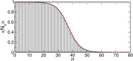
Figure 7: Average distribution of atoms of the first component calculated during the evolution in the presence of collisions. Solid line - fit of the thermal distribution.

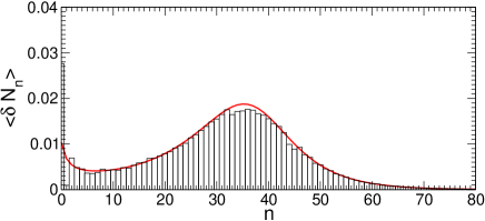
Figure 8: Fluctuations of the atomic distribution for the first component, calculated during the evolution in the presence of collisions. Solid line - fluctuations of the thermal gas with the temperature and the chemical potential determined from the fit of the mean distribution.

Let us now discuss the results calculated with the inclusion of the cooling mechanism. The time dependence of the temperature for the cooling of the two-component gas of fermions is presented in Figure 9. The inset shows the number of fermions as a function of time. The initial state of the system is given by a thermal distribution with temperature $T_{0}=T_{F}$. As for the case of single component Fermi gas, the cooling process was divided into three stages, each consisting of a sequence of two Raman pulses. The pulses that are used are characterized by the following parameters: detuning $\delta/\omega=\{(-11,-12)$, $(-16,-17)$, $(-19,-20)\}$ respectively, Rabi frequency $\Omega/\gamma=\{(0.113,0.113)$, $(0.008,0.012)$, $(0.0025,0.004)\}$ respectively, and length $\Delta t/\omega^{-1}=\{(250,250)$, $(2000,2000)$, $(4000,4000)\}$ respectively. For the considered parameters, not more than $10\%$ of the atoms is excited during each pulse. As one can observe, a final temperature $T\simeq 0.03T_{F}$ may be reached within $6$ s.

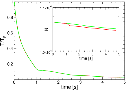
Figure 9: Time-dependence of the temperatures of the two components (darker and lighter curves) during the cooling of a two-component Fermi gas by controlling the effective spontaneous emission rate. Inset: time dependence of the number of atoms. The losses are due to background collisions and the removal of long-living excited atoms. The different Raman cooling stages discussed in the text extend from $0$ $s$ to $1.3$ $s$, from $1.3$ $s$ to $3.2$ $s$, and from $3.2$ $s$ to $5$ $s$.

We have investigated also the statistical properties of the equilibrium distribution in the two-component system, in the presence of both laser-cooling and collisions. The results are presented in Figure 10 (mean occupation numbers) and in Figure 11 (fluctuations). The bars represent the numerical results, calculated by time–averaging during the last stage of the cooling. The solid curves depict the corresponding functions for the thermal distribution, with the temperature and the chemical potential determined from the fit of the average distribution. The mean occupation numbers are exactly the same as predicted by the thermal distribution. The fluctuations in the laser–cooled system, however, are substantially larger than the fluctuations in thermal ensemble. The laser-cooling process induces additional migration of the atoms in the region close to the Fermi energy, leading to the increased fluctuations in this region.

Finally we have studied the storage of the degenerate Fermi gas produced in the cooling process. The main limitation in this case is provided by the background losses, which may generate holes deep within the Fermi sea. The latter increases the corresponding energy per particle, and via collisional thermalization leads to an important source of heating Timmer . We calculate the dynamics of the system, which was already cooled to a temperature $T=0.03T_{F}$. The time dependence of the temperature is presented in Figure 12. The plot compares two cases: (i) the laser is turned off, and the gas is heated due to the background collisions, (ii) the laser is turned on, and the cooling pulses of the last stage are continuously applied. As we may observe from the figure, in the latter case, the laser cooling compensate for the heating induced by the creation of holes in the degenerate distribution. Hence, it helps to maintain the degenerate gas for a relatively long time in the trap. We have also verified that the presence of laser-cooling does not lead to substantially larger losses.

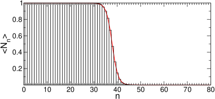
Figure 10: Mean final distribution of fermions (bars) obtained by averaging in time during the last stage of the cooling process presented in Fig. 9. Solid line - fit of the thermal distribution.

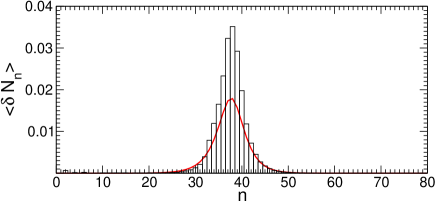
Figure 11: Fluctuations of the final distribution of fermions (bars) obtained by averaging in time during the last stage of the cooling process presented in Fig. 9. Solid line - fluctuations of the thermal gas, with the temperature and the chemical potential determined from the fit of the mean distribution.

V Conclusion

In this paper we have analyzed the laser cooling of trapped one and two-component Fermi gases. We have developed the quantum master equation that describes the laser cooling of fermions, and the process of collisions in the case of the two-component gas. We have considered the FL regime where the heating due to photon reabsorptions can be neglected. We have shown that the inhibition of the spontaneous emission due to Pauli blocking can be overcome employing collective Raman cooling with dynamically modified spontaneous Raman rate. Additionally, a slightly anharmonic trap could be employed. By means of Monte Carlo simulations of the corresponding rate equations, we have shown that it is possible to cool one- and two-component Fermi gases down to temperatures of the order of a few percent of $T_{F}$. The results obtained in this paper present by no means fundamental limits of laser cooling; temperatures below 1% of $T_{F}$ can be achieved by optimizing the cooling procedure TwoComp .

The laser cooling is an external process that influences the dynamics of trapped atoms, therefore one can expect that the equilibrium distribution of the laser-cooled system may differ from the thermal distribution. We have analyzed, both for the single- and the two-component case, the statistics of the laser-cooled gas, comparing the results to the predictions of the grand canonical ensemble. We have shown that although the mean-number distribution can be well approximated by a thermal one, the fluctuations are significantly different. In particular, the fluctuations are considerably enhanced at the Fermi surface. This effect could play a significant role in the BCS pairing in laser cooled gases, and it will be the subject of further analysis.

Additionally, we have discussed the possible loss sources that may affect the laser cooled gas. In particular, for the two-component gas, the creation of holes deep in the Fermi sea due to background collisions could lead to a significant heating of the sample, which should importantly reduce the life-time of the degenerate gas. In this sense, we have shown that our laser-cooling scheme can be employed to maintain a two-component Fermi gas at a fixed temperature without significant additional atom losses.

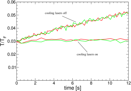
Figure 12: Heating due to background collisions in the degenerate two–component Fermi system. The background collisions rate is assumed to be $\gamma=350$ Hz. The temperature of the system slowly increases when the cooling lasers are turned off. In the presence of the cooling lasers the temperature of the system remain unchanged.

- (1) M. H. Anderson et al., Science 269, 198 (1995); K.B. Davis et al., Phys. Rev. Lett. 75, 3969 (1995); C.C. Bradley et al., ibid 75, 1687 (1995); 79, 1170 (1997).
- (2) B. DeMarco and D. S. Jin, Science 285, 1703 (1999).
- (3) F. Schreck et al, Phys. Rev. Lett. 87, 080403 (2001).
- (4) A.G. Truscott et al., Science 291, 2570 (2001).
- (5) S.R. Granade et al., Phys. Rev. Lett. 88, 120405 (2002).
- (6) Z. Hadzibabic et al., Phys. Rev. Lett. 88, 160401 (2002).
- (7) G. Roati et al., Phys. Rev. Lett. 89, 150403 (2002).
- (8) See e.g. P. G. de Gennes, Superconductivity in metals and alloys, W.A.Benjamin (1966).
- (9) H.T.C. Stoof et al. Phys. Rev. Lett. 76, 10 (1996).
- (10) M. A. Baranov, Yu. Kagan, and M.Yu. Kagan, JETP Lett. 64, 301 (1996).
- (11) M. Houbiers et al., Phys. Rev. A 56, 4864 (1997).
- (12) G.M. Bruun et al., Eur. Phys. J. D 7, 433 (1999).
- (13) M.J. Holland, B. DeMarco, and D.S. Jin, Phys. Rev. A 61, 053610 (2000).
- (14) M. Holland et al., Phys. Rev. Lett. 87, 120406 (2001).
- (15) Y. Ohashi and A. Griffin, Phys. Rev. Lett. 89, 130402 (2002).
- (16) W. Hofstetter et al., Phys. Rev. Lett. 89, 220407 (2002).
- (17) K. M. O’Hara et al., Science 269, 2179 (2002).
- (18) Y. Castin, J. I. Cirac, and M. Lewenstein, Phys. Rev. Lett. 80, 5305 (1998).
- (19) S. Wolf, S.J. Oliver, and D.S. Weiss, Phys. Rev. Lett. 85, 4249 (2000).
- (20) Reduction of reabsorptions has been also observed by C. Salomon (private communication, 1999).
- (21) L. Santos and M. Lewenstein, Phys. Rev. A, 59, 613 (1999).
- (22) L. Santos and M. Lewenstein, Eur. Phys. J. D 7, 379 (1999); L. Santos and M. Lewenstein, Phys. Rev. A 60, 3851 (1999).
- (23) Z. Idziaszek, L. Santos, and M. Lewenstein, Phys. Rev. A 64, 051402 (2001).
- (24) H.T.C. Stoof and M. Houbiers, in Bose-Einstein Condensation in Atomic Gases, Varenna School, 1999, course CXL; L. You and M. Marinescu, Phys. Rev. A 60, 2324 (1999); M.A. Baranov et al., Phys. Rev. A 66, 013606 (2002).
- (25) C. Gardiner, Quantum Noise (Springer-Verlag, Berlin, 1991).
- (26) H.J. Carmichael, Statistical Methods in Quantum Optics 1, (Springer-Verlag, Berlin, 1999).
- (27) Master equation techniques are being cuurently applied by Castin and Carr to study sympathetic cooling of Fermi-Bose mixtures in a cubic box (Y. Castin and L. Carr, private communication, 2002).
- (28) L. Santos and M. Lewenstein, Appl. Phys. B 69, 363 (1999).
- (29) C. Gardiner and P. Zoller, Phys. Rev. A 55, 2902 (1997).
- (30) D. Jaksch, C. W. Gardiner and P. Zoller Phys. Rev. A. 56, 575 (1997).
- (31) I.S. Gradshteyn, I.M. Ryzhik, Table of Intergrals, Series, and Products, (Academic Press, San Diego, 2000).
- (32) M. Holland, J. Williams, and J. Cooper, Phys. Rev. A 55, 3670 (1997).
- (33) Laser cooling of Mg is currently experimentally studied by E. Rasel and W. Ertmer (private communication).
- (34) In particular, it would be difficult to realize the festina lente cooling for very large Lamb-Dicke parameters (), since the smallness of , could set unfeasible requirements on .
- (35) E. Timmermans, Phys. Rev. Lett. 87, 240403 (2001).
- (36) M. Machholm, P.S. Julienne, and K.-A. Suominen, Phys. Rev. A 59, R4113 (1999).
- (37) B. DeMarco et al., Phys. Rev. Lett. 82, 4208 (1999).
- (38) Z. Idziaszek et al., cond-mat/0212538 (2002).