Maximum Fidelity Retransmission of Mirror Symmetric Qubit States

Abstract

In this paper we address the problem of optimal reconstruction of a quantum state from the result of a single measurement when the original quantum state is known to be a member of some specified set. A suitable figure of merit for this process is the fidelity, which is the probability that the state we construct on the basis of the measurement result is found by a subsequent test to match the original state. We consider the maximisation of the fidelity for a set of three mirror symmetric qubit states. In contrast to previous examples, we find that the strategy which minimises the probability of erroneously identifying the state does not generally maximise the fidelity.

1 Introduction

The principles governing communication through a quantum channel have been extensively studied. The transmitting agent, conventionally called Alice, selects a state from a predefined set {$|\psi_{j}\rangle$} with relative frequency $p_{j}$ and transmits a quantum system prepared in this state through the quantum channel. The classical information that is Alice’s message is encoded on a string of such states. The receiving agent, conventionally called Bob, knows the set of states {$|\psi_{j}\rangle$} and their relative frequencies $p_{j}$ which are the prior probabilities he assigns to the states before he makes a measurement. Bob must make a measurement on the states he receives to attempt to recover the encoded information.

The problem for Bob is to determine the best measurement to make. Which measurement is best will depend on how the results are to be used, that is how the information was encoded or what question about the signal states the measurement is designed to answer. For each such coding or question one can define a mathematical ‘figure of merit’ function which provides a measure of how appropriate a given measurement strategy is. Bob’s task in finding his optimal measurement is to maximise this function with respect to all possible measurements. Commonly considered examples of this are the minimum error probability (or minimum Bayes cost) [1, 2, 3, 4] and the accessible information [4, 5, 6, 7], both of which describe recovery of classical information about the original message.

For some applications, Bob needs to use his measurement result to reproduce the quantum signal. The objective is then that the new signal matches the original as closely as possible. We must now consider optimal strategies for the combined measurement and reconstruction process. The quality of these measurement-retransmission strategies is associated with the fidelity $F$. This is the probability that a subsequent measurement on the retransmitted state will confirm that it matches the original signal. The fidelity is a measure of the recovery of quantum information about the state of the signal rather than classical information about the original message.

One motivation for this discussion of the fidelity is the well known question of eavesdropping in quantum communication. Here a third hostile party (conventionally called Eve) wishes to measure the signal coming from Alice and transmit a new signal to Bob which matches the original as closely as possible. Then the error probability or the accessible information of the measurement strategy describes how much Eve expects to gain from eavesdropping, but the fidelity determines the probability that her interception of the signal is undetected. In cryptographic key distribution problems Eve has additional options such as an imperfect cloning and delayed measurement strategy, to take advantage of the extra information available when the preparation basis is announced. It is obviously more appropriate to consider the cloning fidelity [8, 9] than the retransmission fidelity for such strategies.

No general condition is known for maximising the fidelity of a measurement and retransmission strategy, but the maximum fidelity has been found for specific cases [10, 11]. These cases are when the possible signals form a set of symmetric qubit states [10], and where there are only two possible signal qubit states [11]. For these cases the measurement strategy which minimises the probability of incorrectly identifying the states always maximises the fidelity for the best choice of retransmission states. This optimal strategy is not, however, unique for sets of three or more symmetric states.

It is interesting to ask whether the strategy that minimises the error probability always maximises the fidelity. If this is the case then our best strategy is to identify the original signal state as well as we can and then select a corresponding retransmission state. In this paper we establish that the fidelity is not always maximised by the strategy which minimises the probability of erroneously identifying the signal state. We demonstrate this by maximising the fidelity for the mirror-symmetric qubit states for which the minimum error strategy has recently been derived [12].

2 Fidelity

The previous work on maximum fidelity for symmetric states [10] established some important results which we shall make use of. We shall use the notation contained in that work. The signal states are denoted by $|\psi_{j}\rangle$ with associated prior probabilities $p_{j}$ and the retransmission states are $|\phi_{k}\rangle$. The measurement is described by its Probability Operator Measure (POM) elements $\hat{\Pi}_{k}$. These POM elements are operators which represent the probability of occurrence of each possible outcome of a measurement. The probability $P(k|j)$ of the outcome $k$ occurring given that the system was prepared in the state $|\psi_{j}\rangle$ is

$$P(k|j)=\langle\psi_{j}|\hat{\Pi}_{k}|\psi_{j}\rangle.$$ (1)

For the POM elements $\hat{\Pi}_{k}$ to represent probabilities, they must be subject to the following constraints:

1. All the $\hat{\Pi}_{k}$’s are Hermitian.

2. Their eigenvalues are non-negative.

3. The total probability of all outcomes for any input sums to 1:

   $$\sum_{k}\hat{\Pi}_{k}=\hat{1}.$$ (2)

To find the optimal measurement-retransmission strategy we need to express the fidelity $F$ as a function of the POM elements $\hat{\Pi}_{k}$, the retransmission states $|\phi_{k}\rangle$ and the set of possible signal states $\{|\psi_{j}\rangle,p_{j}\}$. The fidelity is the probability that the state $|\phi_{k}\rangle$ selected on the basis of the measurement outcome $\hat{\Pi}_{k}$ will pass a test of the question ‘Is the state $|\psi_{i}\rangle$?’. This test is described by the POM { $|\psi_{i}\rangle\langle\psi_{i}|,\hat{1}-|\psi_{i}\rangle\langle\psi_{i}|$}, where $|\psi_{i}\rangle$ is the state of the original signal. Thus $F$ is given by

$$F=\sum_{j,k}|\langle\psi_{j}|\phi_{k}\rangle|^{2}\langle\psi_{j}|\hat{\Pi}_{k}|\psi_{j}\rangle p_{j}.$$ (3)

This can be written as [10, 11]

$$F=\sum_{k}\langle\phi_{k}|\hat{O}_{k}|\phi_{k}\rangle,$$ (4)

where the positive operator $\hat{O}_{k}$ is given by

$$\hat{O}_{k}=\sum_{j}|\psi_{j}\rangle\langle\psi_{j}|\hat{\Pi}_{k}|\psi_{j}\rangle\langle\psi_{j}|p_{j}.$$ (5)

It is clear from this that the optimal retransmission states $|\phi_{k}\rangle$ are the eigenvectors of the operators $\hat{O}_{k}$ corresponding to the largest eigenvalue $\nu_{k_{+}}$ of $\hat{O}_{k}$.

If these optimal retransmission states are used, then the fidelity is given by the sum of the largest eigenvalues of the $\hat{O}_{k}$ operators:

$$F=\sum_{k}\nu_{k_{+}}$$ (6)

and we need only consider the maximisation of the largest eigenvalues of $\hat{O}_{k}$, subject to the constraint that the operators $\hat{\Pi}_{k}$ form a POM. In such a maximisation each of the POM elements $\hat{\Pi}_{k}$ can be assumed to be proportional to a pure state projector, since the action of any mixed-state like element here would be identical to that of a number of rank 1 POM elements corresponding to the same retransmission state.

3 Mirror Symmetric States

We have recently described the minimum error strategy for a qubit which is known to be one of a set of three mirror symmetric qubit states [12]. Here mirror symmetric means that the set of states is invariant under the transformation

$$|+\rangle\longrightarrow+|+\rangle,\ |-\rangle\longrightarrow-|-\rangle,$$ (7)

with the prior probabilities associated with any mirror-symmetric pair of states being equal.

The set of three mirror symmetric qubit states can be written as

$$|\psi_{1}\rangle = \cos{\theta}|+\rangle+\sin{\theta}|-\rangle,\ p_{1}=p,$$

$$|\psi_{2}\rangle = \cos{\theta}|+\rangle-\sin{\theta}|-\rangle,\ p_{2}=p,$$

$$|\psi_{3}\rangle = |+\rangle,\ p_{3}=1-2p;$$ (8)

where $0\leq\theta\leq\frac{\pi}{2}$ and $0\leq p\leq\frac{1}{2}$.

The minimum error strategy was found to be of different form in two distinct domains of $p$ and $\theta$. The solutions in these two domains are:
for

$$p\geq\frac{1}{2+\cos{\theta}(\cos{\theta}+\sin{\theta})}$$ (9)

the minimum error measurement strategy is given by

$$\hat{\Pi}_{1} = \frac{1}{2}(|+\rangle+|-\rangle)(\langle+|+\langle-|),$$

$$\hat{\Pi}_{2} = \frac{1}{2}(|+\rangle-|-\rangle)(\langle+|-\langle-|),$$

$$\hat{\Pi}_{3} = 0;$$ (10)

and for

$$p\leq\frac{1}{2+\cos{\theta}(\cos{\theta}+\sin{\theta})}$$ (11)

the minimum error measurement strategy is given by

$$\hat{\Pi}_{1} = \frac{1}{2}(a|+\rangle+|-\rangle)(a\langle+|+\langle-|),$$

$$\hat{\Pi}_{2} = \frac{1}{2}(a|+\rangle-|-\rangle)(a\langle+|-\langle-|),$$

$$\hat{\Pi}_{3} = (1-a^{2})|+\rangle\langle+|,$$ (12)

where $a$ is the following function of $p$ and $\theta$:

$$a=\frac{p\cos{\theta}\sin{\theta}}{1-p(2+{\cos}^{2}{\theta})}.$$ (13)

At the boundary between the two domains, which is when the equality holds in the condition (9), $a=1$ and thus $\hat{\Pi}_{3}=0$.

4 Maximising Fidelity for the Mirror Symmetric States

To find the maximum fidelity for the mirror symmetric states we will follow a similar method to that used for the symmetric states [10]. We attempt to write an explicit formula for the fidelity in terms of some parameter set and find the maximum by differentiation.

To maximise the fidelity for these mirror symmetric states we choose a representation of the operator $\hat{O}_{k}$ and find its eigenvalues. To do this we first obtain a general representation of the qubit POM elements. As we stated in section 2 we need only consider elements of rank 1, that is elements proportional to pure state projectors.

The elements of such a POM can be represented by the matrices

$$\hat{\Pi}_{k}=w_{k}\left(\begin{array}[]{cc}1+\cos{\theta_{k}}&\sin{\theta_{k}}e^{i\phi_{k}}\\ \sin{\theta_{k}}e^{-i\phi_{k}}&1-\cos{\theta_{k}}\end{array}\right);$$ (14)

where the basis vectors are

$$|+\rangle=\left(\begin{array}[]{c}1\\ 0\end{array}\right),|-\rangle=\left(\begin{array}[]{c}0\\ 1\end{array}\right);$$ (15)

and $0\leq w_{k}\leq\frac{1}{2}$, $-\pi<\theta_{k}\leq\pi$, $-\frac{\pi}{2}<\phi_{k}\leq\frac{\pi}{2}$.

These POM elements are automatically Hermitian and positive. The remaining completeness constraint (2) becomes equations for $w_{k}$, $\theta_{k}$ and $\phi_{k}$:

$$1-\sum_{k}w_{k}=0,$$ (16)

$$\sum_{k}w_{k}\cos{\theta_{k}}=0,$$ (17)

$$\sum_{k}w_{k}\sin{\theta_{k}}e^{i\phi_{k}}=0.$$ (18)

The operators $\hat{O}_{k}$ for the set of three mirror symmetric states become

$$\hat{O}_{k}=w_{k}\left(\begin{array}[]{cc}\begin{array}[]{c}{2p{\cos}^{2}{\theta}(1+\cos{2\theta}\cos{\theta_{k}})}\\ {+(1-2p)(1+\cos{\theta_{k}})}\end{array}&{p{\sin}^{2}{2\theta}\sin{\theta_{k}}\cos{\phi_{k}}}\\ &\\ {p{\sin}^{2}{2\theta}\sin{\theta_{k}}\cos{\phi_{k}}}&{2p{\sin}^{2}{\theta}(1+\cos{2\theta}\cos{\theta_{k}})}\end{array}\right).$$ (19)

The eigenvalues $\nu_{k_{\pm}}$ of this matrix are given by

$$\begin{array}[]{lcl}\frac{\nu_{k_{\pm}}}{w_{k}}&=&{p(1+\cos{2\theta}\cos{\theta_{k}})+(\frac{1}{2}-p)(1+\cos{\theta_{k}})}\\ &&{\pm[(p\cos{2\theta}(1+\cos{2\theta}\cos{\theta_{k}})+(\frac{1}{2}-p)(1+\cos{\theta_{k}}))^{2}}\\ &&{+p^{2}{\sin}^{4}{2\theta}{\sin}^{2}{\theta_{k}}{\cos}^{2}{\phi_{k}}}]^{\frac{1}{2}},\end{array}$$ (20)

of which the greater eigenvalue is clearly $\nu_{k_{+}}$.

From the form of these eigenvalues we see that the fidelity $F$ is not a function of $\sin{\theta_{k}}$. This means that any element with the parameters $(w_{k},\theta_{k},\phi_{k})$ gives the same contribution to the fidelity as would an element with the parameters $(w_{k},-\theta_{k},\phi_{k})$, and thus the same contribution as the pair of elements $(\frac{w_{k}}{2},\theta_{k},\phi_{k})$ and $(\frac{w_{k}}{2},-\theta_{k},\phi_{k})$. Thus we can replace all of the elements in a POM with such pairs of elements without changing the fidelity, and we need only find the maximum fidelity for POMs consisting of such pairs. Such POMs satisfy condition (18) automatically. Since there is now no condition restricting our choice of $\phi_{k}$, we are free to select $\phi_{k}$ to maximise each eigenvalue $\nu_{k_{+}}$ independently. It is clear from examination of (20) that the best choice is always $\phi_{k}=0$ and thus $\cos{\phi_{k}}=1$. In truth we should have expected such a symmetry of our measurement strategy, since this simply corresponds to the POM also being both mirror symmetric and confined to the plane of the states {$|\psi_{j}\rangle$}.

Since the pair of elements corresponding to $\pm\theta_{k}$ are equally weighted and each contributes the same amount to the fidelity, we now use the parameter $w_{k}$ to represent the combined weight of the pair of elements with the same value of $\cos{\theta_{k}}$.

We can then write the eigenvalues as

$$\nu_{k_{+}}=w_{k}\left[{p\left(1+\cos{2\theta}\cos{\theta_{k}}\right)+\left(\frac{1}{2}-p\right)\left(1+\cos{\theta_{k}}\right)+Q_{k}^{\frac{1}{2}}}\right],$$ (21)

where the functions $Q_{k}$ are given by

$$\begin{array}[]{lcl}Q_{k}&=&\left[p\cos{2\theta}\left(1+\cos{2\theta}\cos{\theta_{k}}\right)+\left(\frac{1}{2}-p\right)\left(1+\cos{\theta_{k}}\right)\right]^{2}\\ &&+p^{2}\sin^{4}{2\theta}\sin^{2}{\theta_{k}}.\end{array}$$ (22)

The POM constraints (16, 17) allow us to simplify the fidelity $F$:

$$F=\sum_{k}\nu_{k_{+}}=\frac{1}{2}+\sum_{k}w_{k}Q_{k}^{\frac{1}{2}}.$$ (23)

To find the stationary points of $F$, subject to the constraints (16, 17) on $w_{k}$ and $\theta_{k}$ we shall use Lagrange’s method of undetermined multipliers. We can construct the function $G$:

$$G=F+\alpha_{1}\left(1-\sum_{k}w_{k}\right)+\alpha_{2}\left(\sum_{k}w_{k}\cos{\theta_{k}}\right),$$ (24)

with the constraint (18) being irrelevant since this $F$ depends on neither $\sin{\theta_{k}}$ nor $\phi_{k}$. The full detail of the maximisation calculation can be found in appendix A, but the main points are summarised here.

The equation $\frac{\partial G}{\partial\theta_{k}}=0$ has four solutions for $\theta_{k}$: $\theta_{k}=0,\pi$ and $\pm\Omega$, where $\Omega$ is some angle depending on the unknown multiplier $\alpha_{2}$. This limits the number of elements in any optimal POM to four.

The minimum value of $w_{k}$, $w_{k}=0$, clearly corresponds to trivial zero operators. The maximum value of $w_{k}$ for a mirror symmetric pair of elements arises from the positivity of the POM elements and the completeness condition (2). These conditions impose a tight bound on $\langle+|\hat{\Pi}_{k}|+\rangle$ and $\langle-|\hat{\Pi}_{k}|-\rangle$, and thus on $w_{k}$. If this bound is reached, then there can be only one other element in the POM, which must be proportional to either $|+\rangle\langle+|$ or $|-\rangle\langle-|$ to satisfy the completeness condition. Thus, if the optimal measurement strategy is composed of more than three elements, then all of the elements must satisfy the equation $\frac{\partial G}{\partial w_{k}}=0$ as well as $\frac{\partial G}{\partial\theta_{k}}=0$.

It is possible to show that there are no values of the unknown multipliers $\alpha_{1}$ and $\alpha_{2}$ which simultaneously satisfy $\frac{\partial G}{\partial w_{k}}=0$ for all four solutions of $\frac{\partial G}{\partial\theta_{k}}=0$, except in special cases where $F$ does not depend on $\theta_{k}$ (for $\cos{\phi}_{k}=1$).

Having established that the optimal strategy consists of three or less elements we simplify the problem by applying the POM conditions (16) and (17) to obtain the most general three element mirror symmetric POM. This POM has only one free parameter, $\cos{\Omega}$, and it is now a simple matter to maximise $F$. The optimal measurement strategy is always found to be one or other of the two mirror symmetric two element strategies.

Obtaining the optimal retransmission states is simply a matter of finding the eigenvector of $\hat{O}_{k}$ corresponding to the larger of its two eigenvalues. The determination of these states is detailed in appendix B.

5 Complete Maximum Fidelity Strategy

We summarise the results for the measurement-retransmission strategy maximising the fidelity for a set of three mirror symmetric states.

If

$$p(1-\cos{2\theta})[p(1-\cos{2\theta})+\cos{2\theta}]=0,$$ (25)

then any POM consisting of elements of the form:

$$\hat{\Pi}_{k}=w_{k}\left(\begin{array}[]{cc}1+\cos{\theta_{k}}&\sin{\theta_{k}}\\ \sin{\theta_{k}}&1-\cos{\theta_{k}}\end{array}\right);$$ (26)

which satisfies the POM conditions (16, 17, 18) with $\phi_{k}=0$, will maximise the fidelity. The optimal retransmission state for each element is then given by

$$|\phi_{k}\rangle=\left({Y_{k}}^{2}+1\right)^{-\frac{1}{2}}(|+\rangle+Y_{k}|-\rangle),$$ (27)

with $Y_{k}$ given by equation (62).

If

$$p\ <\ -\frac{\cos{2\theta}}{1-\cos{2\theta}},\ p\ \neq\ 0,$$ (28)

then the unique optimal measurement strategy consists of the two elements:

$$\hat{\Pi}_{0} = |+\rangle\langle+|$$

$$\hat{\Pi}_{\pi} = |-\rangle\langle-|,$$ (29)

and the optimal retransmission state is $|+\rangle$ if the result is $\hat{\Pi}_{0}$ and $|-\rangle$ if the result is $\hat{\Pi}_{\pi}$.

If

$$p\ >\ -\frac{\cos{2\theta}}{1-\cos{2\theta}},\ p\ \neq\ 0,\cos{2\theta}\ \neq\ 1,$$ (30)

then the unique optimal measurement strategy consists of the two elements:

$$\hat{\Pi}_{+\frac{\pi}{2}} = \frac{1}{2}(|+\rangle+|-\rangle)(\langle+|+\langle-|)$$

$$\hat{\Pi}_{-\frac{\pi}{2}} = \frac{1}{2}(|+\rangle-|-\rangle)(\langle+|-\langle-|),$$ (31)

with the optimal retransmission state for these elements given by

$$|\phi_{\pm\frac{\pi}{2}}\rangle=\left[1+(\sqrt{{\eta}^{2}+1}-\eta)^{2}\right]^{-\frac{1}{2}}\left[|+\rangle\pm(\sqrt{{\eta}^{2}+1}-\eta)|-\rangle\right],$$ (32)

where $\eta$ is given by

$$\eta=\frac{2p\cos{2\theta}+1-2p}{2p\sin^{2}{2\theta}}.$$

6 Comments on the Optimal Strategy

There are only two POMs, (29) and (31), consisting of two pure state projector elements which are mirror symmetric and confined to the plane of the original states. At least one of these two POMs will always be the optimal measurement strategy. The other will give least fidelity of all POMs composed of elements in that plane. In the case where these two give the same fidelity, that is when condition (25) holds, any measurement strategy composed of elements in that plane will also be optimal. This condition (25) can be decomposed into to two obvious cases and one intriguing case. The first two are when there is only one possible signal state ($p=0$) and when all of the signal states are identical ($\theta=0$). The remaining case corresponds to the situation that the sum of the density matrices of the states, each multiplied by the probability of NOT selecting that state, sums to the identity matrix, as described by the equation

$$\sum_{j}(1-p_{j})|\psi_{j}\rangle\langle\psi_{j}|=\hat{1}.$$ (33)

The meaning of this final condition remains unclear.

The retransmission states $|\phi_{k}\rangle$ for the $\theta_{k}=0,\pi$ solution are simple to understand as they are just the states that the POM elements project on to. The origin of the retransmission states for the $\theta_{k}=\pm\frac{\pi}{2}$ case seems less transparent, but they are simply the states that the POM elements project onto, rotated to increase their overlap with the a priori state of the signal.

We wish to compare the optimal measurement strategy for maximum fidelity with that for minimum error. The $\theta_{k}=0,\pi$ strategy is never optimal for distinguishing between three mirror symmetric states with least probability of error. The POM given by $\theta_{k}=\pm\frac{\pi}{2}$ is the strategy which distinguishes $|\psi_{3}\rangle$ and $|\psi_{2}\rangle$ (the mirror symmetric pair) with minimum error probability. This strategy is optimal for distinguishing some mirror symmetric sets of states with least error. These sets are given by the condition (9). This equation (9) bears little resemblance to the condition (30) for the $\theta_{k}=\pm\frac{\pi}{2}$ strategy being the optimal fidelity measurement, save that both are satisfied for larger values of $p$. This is to be expected as we know from [10, 11] that the optimal strategies must coincide for two equiprobable states, that is for $p=\frac{1}{2}$. The domains in which these strategies are optimal, and the boundaries between them are shown in figure 1.

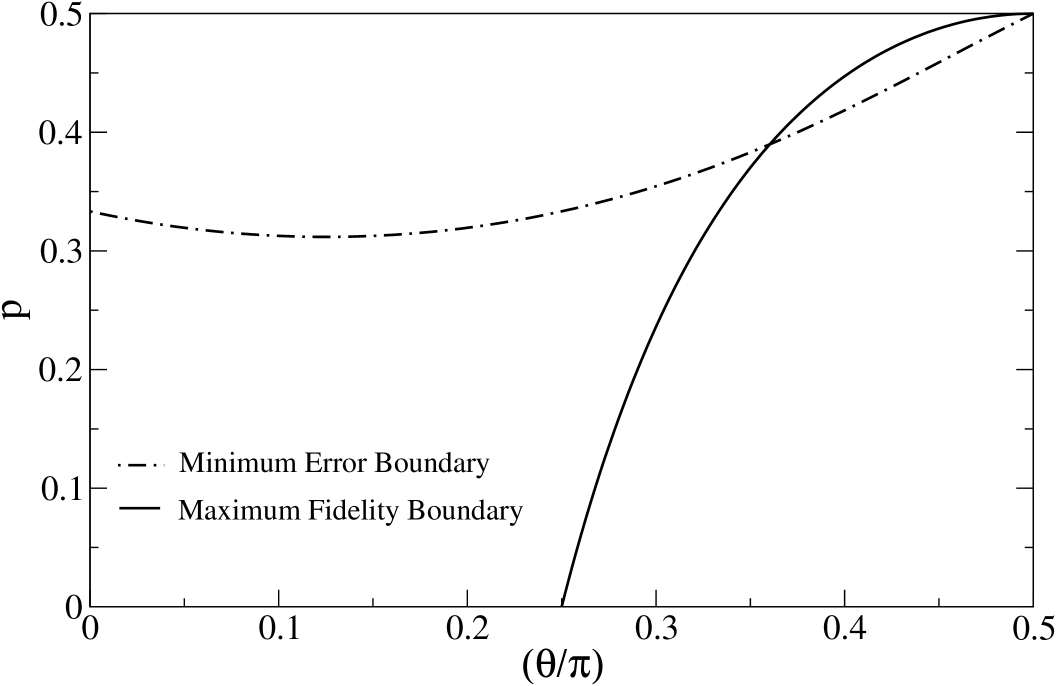
Figure 1: A comparison of the domains in which the $\theta_{k}=\pm\frac{\pi}{2}$ strategy is optimal for minimum error [equation (9), above the dash-dot line] and for maximum fidelity [equation (30), to the left of the solid line], in terms of the state parameters $p$ and $\theta$.

From this diagram we can see that the region where $\theta_{k}=\pm\frac{\pi}{2}$ is the fidelity maximising measurement strategy (left of the solid line) contains most of the region where this POM is the minimum error measurement strategy (above the dot-dash line). There is, however, a sizable region where the $\theta_{k}=\pm\frac{\pi}{2}$ strategy maximises the fidelity without minimising the error probability and a smaller region where it minimises the error probability without maximising the fidelity.

It could be argued that the lack of correlation should not surprise us, as the two boundaries have very different significance. The boundary (9) for the minimum error strategy shows where the two element (10) and three element (12) strategies are identical in form, and the two element strategy is only optimal when one of the three elements given by (12) is not a positive operator. Conversely the boundary for optimal fidelity strategies corresponds to the situation where the two very different strategies which are optimal in their respective domains give the same fidelity. The fidelity is generally maximised by a two element strategy.

There is a unique strategy minimising the probability of error for all possible mirror symmetric sets of three qubit states, and a unique fidelity maximising strategy everywhere not on the solid boundary in figure 1. Since these unique strategies coincide only in the region of figure 1 to the left of the solid line and above the dot-dash line, it is clear that the minimum error strategy does not generally maximise the fidelity.

Two of the previous solutions [10, 11] for a strategy maximising fidelity for a certain class of state sets overlap somewhat with the mirror symmetric states. The case of two equiprobable pure states clearly just corresponds to our mirror symmetric states with $p=\frac{1}{2}$. Unsurprisingly our solution is in complete agreement with [10, 11] in predicting that fidelity is maximised by the minimum error measurement strategy in this case. The second case is that of the Trine states, an example of a set of symmetric states which is also dealt with in [10]. Their solution predicts that any POM with elements in the common plane of the three Trine states will be optimal. It is easy to show that the Trine states, with $p=\frac{1}{3}$ and $\theta=60^{o}$, satisfies the equality (59), and hence also (25), and thus our solution is also in accord here. It is interesting to note that we predict the same solution for a much wider class of state sets than just the Trine states, so it may be possible to extend the solution for the general set of symmetric states to a broader class of sets.

Finally, in the course of the solution for a set of three mirror symmetric states we only referred to the nature and number of the states themselves in finding the eigenvalues of our $\hat{O}_{k}$ matrices. The only property of these eigenvalues that we used in deriving our solution was that the sum of them depended only on the values of $\cos{\theta_{k}}$ and ${\cos}^{2}{\phi_{k}}$, and not otherwise on $\sin{\theta_{k}}$ or $\phi_{k}$. The rest of the analysis was done using the coefficients of $\cos{\theta}_{k}$ ($A$, $B$ and $C$ in the appended calculations) and holds true for any form of these coefficients. This implies that for any set of qubit states for which this eigenvalue sum has a similar dependence only on $\cos{\theta_{k}}$ and ${\cos}^{2}{\phi_{k}}$, the optimal measurement strategy will again be either $\theta_{k}=\{\pm\frac{\pi}{2}\}$ or $\theta_{k}=\{0,\pi\}$, or any set of elements in the linear plane if the fidelity of these two strategies is the same. In particular this means our strategy maximising the fidelity for a set of three mirror symmetric states is also the measurement strategy for maximising the fidelity for any number of mirror symmetric states sharing a common plane. The form of the condition (59) will obviously become more complex in terms of the original variables when there are more states, but will be unchanged as a function of the coefficients of $\cos{\theta_{k}}$ (54).

7 Conclusions

The fidelity of a measurement and reconstruction strategy is defined as the average probability that a subsequent measurement on the reconstructed state will identify it as being identical to the original state. We sought to find a strategy which maximised the fidelity for a mirror symmetric set of three qubit states. This was done by parameterising the POM, evaluating the fidelity as a function of these parameters and conducting a variational calculation using Lagrange’s method of undetermined multipliers to identify the sets of elements which could constitute the maximum.

The optimal measurement strategy was found to be whichever of the two mirror symmetric two element POMs gives the larger fidelity for a given set of states, and that any POM whose elements lie in the plane of the states is optimal if these two strategies give the same fidelity. The optimal retransmission states were found using an eigenvector equation (61).

Unlike all previous solutions for maximum fidelity strategies, the minimum error measurement strategy does not generally maximise the fidelity of a set of mirror symmetric states.

Appendix A Derivation of the Fidelity Maximising Measurement

In attempting to maximise the fidelity $F$ subject to the POM conditions (16, 17) it is helpful to begin by using Lagrange’s method of undetermined multipliers. We construct the function $G$:

$$G=F+\alpha_{1}\left(1-\sum_{k}w_{k}\right)+\alpha_{2}\left(\sum_{k}w_{k}\cos{\theta_{k}}\right).$$ (34)

Varying $G$ with respect to $w_{k}$ gives us a restriction on the possible positions of the global maxima and minima of $G$, which must be located either at a stationary point with respect to $w_{k}$:

$$\frac{\partial G}{\partial w_{k}}=Q_{k}^{\frac{1}{2}}-\alpha_{1}+\alpha_{2}\cos{\theta_{k}}=0,$$ (35)

or at the maximum or minimum possible values of $w_{k}$:

$$w_{k:min}=0,\ \ w_{k:max}=\frac{1}{1+|\cos{\theta}_{k}|};$$ (36)

with this maximum arising from the fact that $w_{k}$ represents the combined weight of the pair of POM elements corresponding to $\pm{\theta}_{k}$, and that the component of such a pair in either the $|+\rangle$ or $|-\rangle$ direction cannot exceed 1. The minimum value of $w_{k}$ clearly corresponds to trivial zero operators.

Since $Q_{k}$ is a function of $\cos{\theta_{k}}$ only, differentiating $G$ with respect to $\theta_{k}$ gives

$$\frac{\partial G}{\partial\theta_{k}}=\frac{w_{k}}{2}Q_{k}^{-\frac{1}{2}}\frac{\partial Q_{k}}{\partial\cos{\theta_{k}}}(-\sin{\theta_{k}})-\alpha_{2}w_{k}\sin{\theta_{k}}=0$$ (37)

at a stationary point of $G$. This has the nontrivial solutions:

$$\sin{\theta_{k}}=0\ =>\ \theta_{k}=0\ or\ \pi$$ (38)

and

$$\frac{\partial Q_{k}}{\partial\cos{\theta_{k}}}=-2\alpha_{2}Q_{k}^{\frac{1}{2}},$$ (39)

as well as the $w_{k}=0$ solution corresponding to the element not being part of the POM.

To simplify further analysis we shall assign the coefficients of $\cos{\theta_{k}}$ in $Q_{k}$ to be

$$A=p\cos{2\theta}+\left(\frac{1}{2}-p\right),$$

$$B=p\sin^{2}{2\theta}=\frac{1}{2}-C\ \geq\ 0,$$

$$C=p\cos^{2}{2\theta}+\left(\frac{1}{2}-p\right)=\frac{1}{2}-B\ \geq\ 0;$$

so that $Q_{k}$ is given by

$$Q_{k}=(A+C\cos{\theta_{k}})^{2}+B^{2}(1-\cos^{2}{\theta_{k}}).$$

We can then solve equation (39) to find the remaining values of $\theta_{k}$ which satisfy $\frac{\partial G}{\partial\theta_{k}}=0$. Since equation (39) contains only $\cos{\theta_{k}}$ terms, it is simplest to express the solution as a value of $\cos{\theta_{k}}$ given in terms of our $A,B,C$ coefficients as

$$\cos{\theta_{k}}=\frac{1}{C^{2}-B^{2}}\left(-AC-\alpha_{2}B\sqrt{\scriptstyle{\frac{A^{2}+B^{2}-C^{2}}{\alpha_{2}^{2}+B^{2}-C^{2}}}}\right),$$ (40)

which can only take one value for a given POM since $\alpha_{2}$ must have a single value for all of the elements of one POM.

We can now say that any measurement maximising the fidelity has at most four elements, corresponding to the four solutions of $\frac{\partial G}{\partial\theta_{k}}=0$ (37) for $\theta_{k}$, given by equations (38) and (40). For each of these possible elements, either equation (35) holds (a stationary point of $G$ with respect to $w_{k}$) or $w_{k}$ takes its maximum or minimum value.

Now we must consider whether it is possible to have all four of these elements present in one POM, i.e. that none of the weight factors $w_{k}$ are zero for these elements. Clearly this implies that none of them take their maximum values either, since the maximum value of $w_{k}$ for an element (or mirror symmetric pair of elements) is found by noting that the positivity and completeness of the POM implies that neither the $|+\rangle\langle+|$ or $|-\rangle\langle-|$ component of any element (or pair) can exceed 1. If any element saturates this bound, there can be only one more nonzero element corresponding to either $|+\rangle\langle+|$ or $|-\rangle\langle-|$ to satisfy the completeness condition (2).

Since no weight factor $w_{k}$ can attain its maximum value when there are four nonzero elements present in the POM, the equation (35) must be simultaneously satisfied for all four elements. This occurs if there is a pair of values for $\alpha_{1}$ and $\alpha_{2}$ which will satisfy (35) for all three solutions for $\cos{\theta_{k}}$ obtained from (37).

For $\theta_{k}=0$ and $\pi$, equation (35) gives

$$\theta_{k}=0:|A+C|=\alpha_{1}-\alpha_{2},$$ (41)

$$\theta_{k}=\pi:|A-C|=\alpha_{1}+\alpha_{2},$$ (42)

which fixes both $\alpha_{1}$ and $\alpha_{2}$ for any measurement strategy containing both of these elements. These values must satisfy the equation (35) for the value of $\cos{\theta_{k}}$ given by (40). Since the multipliers $\alpha_{1}$ and $\alpha_{2}$ can only take the values $\pm A,\mp C$ respectively or $\pm C,\mp A$ respectively for any values of $A$ and $C$ when (41, 42) hold, it is simple to show that equation (35) can only be satisfied for this value of $\cos{\theta_{k}}$ when either

$$A^{2}+B^{2}-C^{2}=0\ \mathrm{or}\ B=0.$$ (43)

Which of these two conditions is relevant depends on the relative magnitudes and signs of $A$ and $C$. Thus we see that we can only have a four element POM in certain special cases.

Examining these special cases shows that in each of them $Q_{k}$ is the square of some linear function of $\cos{\theta_{k}}$ which is either positive for all $\theta_{k}$ or negative for all $\theta_{k}$. If $|Q_{k}^{\frac{1}{2}}|$ is any linear function of $\cos{\theta_{k}}$, it can be shown by application of the POM conditions (16, 17) that $F$ does not depend on any $\cos{\theta_{k}}$ and thus the fidelity is constant for any measurement strategy composed of elements confined to the plane of the states (that is for which $\cos{\phi_{k}}=1$).

For the general case where $F$ does depend on the strategy chosen we now know that there is no strategy composed of four or more elements which can be a maximum or minimum of the fidelity. Denoting the solution of equation (40) in the range $0\ \leq\ \theta_{k}\ \leq\ \pi$ as $\theta_{k}=\Omega$, there are two possibilities for three element strategies: case (i)

$$\theta_{k}=\pi,\pm\Omega;\ 1\ \geq\ \cos{\Omega}\ \geq\ 0;$$ (44)

or case (ii)

$$\theta_{k}=0,\pm\Omega;\ -1\ \leq\ \cos{\Omega}\ \leq\ 0.$$ (45)

Both of the two element measurement strategies which are mirror symmetric in this basis are special cases of these three element strategies, and are located at the edge of the domains of the three element strategies. The $\theta_{k}=\{0,\pi\}$ strategy corresponds to $\cos^{2}{\Omega}=1$ in either of the above cases, and the $\theta_{k}=\{\pm\frac{\pi}{2}\}$ strategy corresponds to $\cos{\Omega}=0$.

For these three element strategies the POM conditions (16) and (17) place a strict limit on the values of the weight factors $w_{k}$. Denoting the weights of the $\theta_{k}=0,\pi$ elements and the $\theta_{k}=\pm\Omega$ pair by $w_{0}$, $w_{\pi}$ and $w_{\Omega}$ respectively, we have either:

(i) for $\cos{\Omega}\ \geq\ 0$

$$w_{\pi}+w_{\Omega}=1,\ w_{\pi}-w_{\Omega}\cos{\Omega}=0$$ (46)

which gives

$$w_{\Omega}=\frac{1}{1+\cos{\Omega}},\ w_{\pi}=\frac{\cos{\Omega}}{1+\cos{\Omega}};$$ (47)

or (ii) for $\cos{\Omega}\ \leq\ 0$

$$w_{0}+w_{\Omega}=1,\ w_{0}+w_{\Omega}\cos{\Omega}=0$$ (48)

which gives

$$w_{\Omega}=\frac{1}{1-\cos{\Omega}},\ w_{0}=\frac{-\cos{\Omega}}{1-\cos{\Omega}}.$$ (49)

Now we need simply differentiate $F$ with respect to $\cos{\Omega}$ for each of these two strategies and select the largest value of $F$ from any stationary points and the two limiting two element strategies. Both of these strategies automatically satisfy all of the POM conditions so we no longer need to use Lagrange’s method of undetermined multipliers.

Case (i):

For the $\theta_{k}=\pi,\pm\Omega$ case the stationarity equation $\frac{\partial F}{\partial\cos{\Omega}}=0$ can be rearranged and squared to obtain

$$B^{2}(C^{2}-B^{2}-A^{2})(1+\cos{\Omega})^{2}=0.$$ (50)

The only solutions to this equation are the aforesaid special cases (43) and $\cos{\Omega}=-1$, which is not allowed since $\cos{\Omega}\ \geq\ 0$ in this case. We conclude that there are no stationary points of $F$ for this set of strategies and the maximum and minimum of the fidelity for these strategies must correspond to the two element strategies which define the end points of our variation (i.e. $\cos{\Omega}=0$ or $1$).

Case (ii):

Similarly for the $\theta_{k}=0,\pm\Omega$ case, $\frac{\partial F}{\partial\cos{\Omega}}=0$ implies that

$$B^{2}(C^{2}-B^{2}-A^{2})(1-\cos{\Omega})^{2}=0.$$ (51)

As before, the only solutions to this are our two special cases (43) and the single value of $\cos{\Omega}=1$, which is not in the domain for this strategy. We can thus conclude that there are no stationary points of $F$ for either strategy and our global maximum and minimum must correspond to the $\theta_{k}=\{\pm\frac{\pi}{2}\}$ and $\theta_{k}=\{0,\pi\}$ strategies which are at the end points of both of our three element strategy domains.

The fidelity for each of the two strategies which must constitute our maximum and minimum are

for $\theta_{k}=\{\pm\frac{\pi}{2}\}$

$$F=\frac{1}{2}+\sqrt{B^{2}+A^{2}},$$ (52)

and for $\theta_{k}=\{0,\pi\}$

$$F=\frac{1}{2}+\frac{|A+C|}{2}+\frac{|A-C|}{2},$$ (53)

which is just equal to a half plus the larger of $|A|$ or $|C|$.

The larger of these two fidelities, (52) and (53), will be the maximum fidelity, and the corresponding POM will be the optimal measurement strategy. For the $\theta_{k}=\{0,\pi\}$ strategy to be optimal, we must have $C\ \geq\ |A|$ since the fidelity of the $\theta_{k}=\{\pm\frac{\pi}{2}\}$ strategy is always at least $\frac{1}{2}+|A|$. Thus the $\theta_{k}=\{0,\pi\}$ strategy is only uniquely optimal if

$$A^{2}+B^{2}-C^{2}\ <\ 0,$$ (54)

which can be restated in terms of the original variables $p$ and $\theta$ as

$$p\ <\ -\frac{\cos{2\theta}}{1-\cos{2\theta}}.$$ (55)

The two strategies give the same fidelity when the relevant condition in (43) holds. This corresponds to the special case where any POM consisting of elements confined to the plane of the states is optimal. These conditions can be written in terms of $p$ and $\theta$ as:

$$p(1-\cos{2\theta})[p(1-\cos{2\theta})+\cos{2\theta}]=0,$$ (56)

that is either

$$p=0,$$ (57)

or

$$\cos{2\theta}=1,$$ (58)

or

$$p=-\frac{\cos{2\theta}}{1-\cos{2\theta}}.$$ (59)

The meaning of two of these three cases is clear: equation (57) is the case where there is only one possible signal state and equation (58) describes the case where all three states are identical. The fidelity obviously cannot depend on the measurement strategy at all in these cases. The third of these cases, equation (59), is less obvious. In fact it corresponds to the identity:

$$\sum_{j}(1-p_{j})|\psi_{j}\rangle\langle\psi_{j}|=\hat{1},$$ (60)

that is when the sum of the density operators of the states normalised to the prior probability of NOT selecting that state is the identity operator.

Appendix B Retransmission States

In equation (4) we found the optimal retransmission states to be the eigenvectors of $\hat{O}_{k}$, which is given by equation (5). This determines the best retransmission state for any measurement we choose to make, not only the optimal measurement. The optimal retransmission state $|\phi_{k}\rangle$ depends on the possible states of the original signal {$|\psi_{j}\rangle$} and on the direction of the corresponding measurement operator $\hat{\Pi}_{k}$. Since $|\phi_{k}\rangle$ does not depend on the weight ($w_{k}$) of this element or on the rest of the POM, $|\phi_{k}\rangle$ will be the optimal retransmission state for any POM containing an element in this direction. This is useful as we need only find $|\phi_{k}\rangle$ for each possible element, without having to consider the strategy in which the element occurs. It could therefore be said that the optimal retransmission state $|\phi_{k}\rangle$ depends on the result of the measurement (given by the direction of $\hat{\Pi}_{k}$) rather than on the measurement strategy (that is the experiment whose outcome was $k$).

It is simplest to find the states {$|\phi_{k}\rangle$} if we consider the folowing three cases separately: $\theta_{k}=0$, $0<|\theta_{k}|<\pi$ and $\theta_{k}=\pi$.

For $\theta_{k}=0$ our $\hat{O}_{k}$ matrix has eigenvectors $|+\rangle$ and $|-\rangle$. The larger eigenvalue belongs to $|+\rangle$ if $A+C>0$. Since we found previously that we must have $C\ \geq\ |A|$ for $\theta_{k}=0,\pi$ to be the best strategy, it is always the case that the optimal retransmission state for the element $\Pi_{0}$ is $|+\rangle$ when we have employed the optimal measurement strategy.

Similarly, for $\theta_{k}=\pi$ our $\hat{O}_{k}$ matrix again has eigenvectors $|+\rangle$ and $|-\rangle$. The larger eigenvalue now belongs to $|-\rangle$ if $A-C<0$, which is again always true when the optimal strategy includes a $\theta_{k}=\pi$ element.

For any other value of $\theta_{k}$, such as $\theta_{k}=\pm\frac{\pi}{2}$, we must find the general solution for the eigenvector corresponding to the larger eigenvalue of a $2\times 2$ real Hermitian matrix. We need only study nondiagonal matrices since the $\hat{O}_{k}$ matrix is diagonal when $\theta_{k}\neq 0$ or $\pi$ only for trivial sets of states {$|\psi_{j}\rangle,p_{j}$}. The equation for the unnormalised eigenvectors is

$$\left(\begin{array}[]{cc}R_{k}&S_{k}\\ S_{k}&P_{k}\end{array}\right)\left(\begin{array}[]{c}1\\ Y_{k\pm}\end{array}\right)=\nu_{k\pm}\left(\begin{array}[]{c}1\\ Y_{k\pm}\end{array}\right)$$ (61)

which gives a value for $Y_{k\pm}$ in terms of the matrix elements:

$$Y_{k\pm}=\frac{P_{k}-R_{k}}{2S_{k}}\pm\frac{\sqrt{(P_{k}-R_{k})^{2}+4S^{2}_{k}}}{2S_{k}},$$ (62)

where the $\pm$ in $Y_{k\pm}$ in this equation corresponds to the two eigenvalues $\nu_{k\pm}$, so the eigenvector of interest is that which contains $Y_{k+}$.

From the general form of $\hat{O}_{k}$ given in equation (19) we can identify the elements of our eigenvector equation as

$$R_{k} = 2p\cos^{2}{\theta}(1+\cos{2\theta}\cos{\theta_{k}})+(1-2p)(1+\cos{\theta_{k}})$$

$$P_{k} = 2p\sin^{2}{\theta}(1+\cos{2\theta}\cos{\theta_{k}})$$

$$S_{k} = p\sin^{2}{2\theta}\sin{\theta_{k}},$$ (63)

from which we can identify $Y_{k+}$ and thus find and normalise $|\phi_{k}\rangle$. It can be readily appreciated that the form of these states is not simple.

For the case where $\theta_{k}=\pm\frac{\pi}{2}$, we identify the parameter $\eta$ as

$$\eta=\frac{R_{k}-P_{k}}{2|S_{k}|}=\frac{2p\cos{2\theta}+(1-2p)}{2p\sin^{2}{2\theta}},$$ (64)

then $Y_{\pm\frac{\pi}{2}}$ is given by

$$Y_{\pm\frac{\pi}{2}}=\pm\left(\sqrt{{\eta}^{2}+1}-\eta\right).$$ (65)

The optimal retransmission state for this strategy is given by

$$|\phi_{\pm\frac{\pi}{2}}\rangle=\frac{1}{\sqrt{1+(Y_{\pm\frac{\pi}{2}})^{2}}}[|+\rangle+(Y_{\pm\frac{\pi}{2}})|-\rangle].$$ (66)

It is clear from the form of $Y_{\pm\frac{\pi}{2}}$ (65) that the retransmission state given by (66) is, as expected, on the same side of the Bloch sphere as the corresponding POM element $\hat{\Pi}_{\pm\frac{\pi}{2}}$. Further analysis of the physical meaning of these states is possible by rewriting the $\eta$ parameter as

$$\eta=\frac{\langle+|\hat{\rho}_{T}|+\rangle-\langle-|\hat{\rho}_{T}|-\rangle}{2p\sin^{2}{2\theta}},$$ (67)

where $\hat{\rho}_{T}$ is the state Bob assigns to the signal before making his measurement and is given by

$$\hat{\rho}_{T}=\sum_{j}p_{j}|\psi_{j}\rangle\langle\psi_{j}|.$$ (68)

It is clear that $\hat{\rho}_{T}$ is also a measure of the ‘average state’ of the signal sent by Alice and that $\eta$ is positive if the $|+\rangle\langle+|$ component of $\hat{\rho}_{T}$ is larger than the $|-\rangle\langle-|$ component (the ‘average state’ is closer to $|+\rangle$ than $|-\rangle$) and negative if the converse is true. Furthermore we see that $|Y_{\pm\frac{\pi}{2}}|$ is larger than one if $\eta$ is negative and smaller than one is $\eta$ is positive, so that the retransmission states $|\phi_{\pm\frac{\pi}{2}}\rangle$ are shifted from $|+\rangle\pm|-\rangle$ towards the ‘average state’, $\hat{\rho}_{T}$.

References

References

- [1] Helstrom C.W. 1976 Quantum Detection and Estimation theory (New York: Academic).
- [2] Holevo A.S. 1982 Probabilistic and Statistical Aspects of Quantum Theory (Amsterdam: North-Holland).
- [3] Yuen H.P., Kennedy R.S. and Lax M. 1975 IEEE Trans. Inf. Theor. IT-21 125.
- [4] Clarke R.B.M., Kendon V.M., Chefles A., Barnett S.M., Riis E. and Sasaki M.; 2001 Phys. Rev. A. 64 012303.
- [5] Davies E.B. 1978 IEEE Trans. Inf. Theor. IT-24 596.
- [6] Sasaki M., Barnett S.M., Jozsa R., Osaki M. and Hirota O.; 1999 Phys. Rev. A. 59 3325.
- [7] Mizuno J., Fujiwara M., Akiba M., Kawanishi T., Barnett S.M., Sasaki M.; 2002 Phys. Rev. A. 65, 012315.
- [8] Gisin N. and Massar S.; 1997 Phys. Rev. Let. 79 2153
- [9] Bruß D., Ekert A. and Machiavello C.; 2000 Phys. Rev. Let. 81 2598
- [10] Barnett S.M., Gilson C.R. , Sasaki M.; 2001 J. Phys. A: Math, Gen 34, 6755.
- [11] Fuchs C.A. and Sasaki M. (private communication).
- [12] Andersson E., Barnett S.M., Gilson C.R., and Hunter K. 2002 Phys. Rev. A. 65, 052308.