Entanglement gauge and the non-Abelian geometric phase with two photonic qubits

Abstract

We introduce the entanglement gauge describing the combined effects of local operations and nonlocal unitary transformations on bipartite quantum systems. The entanglement gauge exploits the invariance of nonlocal properties for bipartite systems under local (gauge) transformations. This new formalism yields observable effects arising from the gauge geometry of the bipartite system. In particular, we propose a non-Abelian gauge theory realized via two separated spatial modes of the quantized electromagnetic field manipulated by linear optics. In this linear optical realization, a bi-partite state of two separated spatial modes can acquire a non-Abelian geometric phase.

I Introduction

At the heart of quantum information theory is the phenomenon of entanglement between spatially separated systems. Nonlocal correlations due to entanglement allow powerful information processes that cannot be performed classically: entanglement is central to tests of local realism Bel64 and is a fundamental resource of quantum teleportation Ben93 , quantum cryptography Eke91 ; Cir97 ; Fuc97 , and possibly quantum computing Bra99 ; Eke98 . Moreover, nonlocal entanglement-generating transformations of multi-partite states can allow for communication Ben92 ; Eis00 and distributed quantum computing Eis00 ; Cir99 . The possibilities of manipulating nonlocal properties using only local operations (e.g., entanglement distillation Ben96 ) are therefore an important resource issue for quantum information.

Here we show that nonlocal properties of quantum states are simplified and isolated through the use of gauge theoretical concepts Egu80 . A powerful tool of modern mathematical physics, gauge theory is used to describe the geometric structure of systems possessing symmetry under specific (gauge) transformations. In quantum mechanics, it is known that local transformations on components of a multi-partite system do not change the entanglement. We show that local operations can be expressed as a form of gauge transformation, which we define as the entanglement gauge. Nonlocal properties such as entanglement, then, are naturally expressed as entanglement gauge invariant quantities. With this entanglement gauge formalism, general transformations on a bi-partite system can be decomposed into nonlocal and local (gauge) transformations. Nonlocal properties can be defined on a generally curved space that is given by an equivalence class of states under local operations.

One manifestation of employing entanglement gauge theory is that, for a given nonlocal transformation on this generally curved space, effects due to geometric phases Ber84 ; Sim83 can arise in non-trivial ways. These phases can arise in many different physical situations Fue02 and may even be utilized as a resource for quantum information processes; of particular interest, it has recently been proposed Jon00 that geometric phases in two-qubit systems can allow for a fault-tolerant conditional phase shift gate in quantum computation. For general systems with more than two qubits, holonomic quantum computation has also been investigated Zan99 .

Current experiments are now at the point where controlled local and nonlocal transformations in a wide variety of physical systems are accessible, and one can observe the manifestations of these geometric phases. Optical realizations offer the advantage of negligible decoherence as well as the advanced ability to implement unitary operations using linear optics. These realizations also provide a natural source of entanglement in parametric down-conversion (PDC), with which photon pairs can be created in a polarization-entangled state Kwi95 . Recent experiments Whi02 have produced a wide selection of two-photon states, with varying degrees of entanglement and disorder (entropy), and have characterized the resulting state using quantum tomography.

Many optical experiments can be described as first producing the photon pairs via PDC (with controllable degrees of entanglement and entropy), and then directing the photons through passive linear optical elements (beam splitters, phase shifters, polarization rotators). Using a setup of this form, Kwiat and Chiao Kwi91 have demonstrated an Abelian geometric phase shift in an (unentangled) two-photon system. The Abelian geometric phase for an entangled or partially-entangled system has been investigated theoretically Sjo00a , and an Abelian geometric phase for mixed states in interferometry has been proposed Sjo00b .

We show in this paper that optical states of a bi-partite system are naturally described in an entanglement gauge formalism. Also, by manipulating such states with linear optical elements, they can acquire a non-Abelian geometric phase (NAGP) Wil84 ; Ana88 . An NAGP arises if instead of a single state vector, which spans a one-dimensional subspace of Hilbert space, the cyclic evolution of a $n$-dimensional subspace is studied. In this case, the usual U(1) geometric phase factor is generalized to geometric U($n$) unitary transformations. The notion of a non-Abelian “phase” is justified because all eigenvalues of unitary operators are phase factors, despite the fact that the resulting transformation on a general state is not simply an additional phase in the traditional sense. We illustrate the concept of a NAGP using quantum interferometry to evolve bi-partite states about a closed loop; the NAGP acquired can be measured using quantum tomography, a technique that can completely characterize our proposed bi-partite states Whi02 . We discuss its relevance in the context of entanglement and quantum information theory.

The paper is structured as follows. In Sec. II, we describe the relevant Hilbert spaces and transformations in quantum interferometry, along with a description of the entanglement gauge structure. We define the NAGP for cyclic evolution in Sec. III, and give a parametrization and explicit expression for the NAGP for the relevant coset space. In Sec. IV, we calculate the NAGP acquired in a quantum interferometry setup for various types of cyclic evolution, giving specific examples. We conclude with Sec. V.

II Photon interferometry

In this section, we review the mathematical structure of two-photon quantum interferometry. This structure allows us to construct the geometrical space describing the entanglement gauge for bi-partite optical states of two photons. (We note that the general formalism developed here can be applied to other physical systems, e.g., trapped ions Cir95 with two phonons. However, working explicitly with an optical realization gives a valuable physical context.)

Consider a two-channel (four-port) optical interferometer with polarization-dependent elements. There are four boson field modes to consider, each with a corresponding annihilation operator: $a_{H}$ corresponding to the horizontal polarization for the $a$ spatial mode, $a_{V}$ corresponding to the vertical polarization for the $a$ spatial mode, and annihilation operators $b_{H},b_{V}$ for the horizontal and vertical polarizations for the $b$ spatial modes. A passive linear optical experiment can employ polarization rotation, beam splitters, phase shifters and mirrors as stages of the processing of the quantum state Bar01 . Each of these stages can be represented mathematically as a unitary transformation provided that losses are neglected. Together, these transformations close to the group $U(4)$; thus, we say that a passive polarization-dependent two channel interferometer invokes a transformation $g\in U(4)$.

For a quantum interferometer, transformations on quantum optical states are given by a representation of $U(4)$. Because passive optical transformations are photon-number-preserving, each irreducible representation (irrep) is labelled by $N$, the total number of photons. That is, the Hilbert space $\mathbb{H}_{N}$ for each irrep $N$ contains the $U(4)$ highest weight state $|\phi_{N}\rangle=\frac{1}{\sqrt{n!}}(a^{\dagger}_{H})^{N}|0\rangle$, where $|0\rangle$ is the Fock state vacuum. This highest weight state is constructed such that all the photons are in channel $a$ with horizontal polarization.

In the following, we define local operations to be those operations that act on the spatial modes $a$ (or $b$) alone, whereas nonlocal operations mix the spatial modes $a$ and $b$ together. Of course, nonlocal operations in $U(4)$ are performed using only spatially local interactions by bringing modes $a$ and $b$ together, such as at a beamsplitter. For our development, however, we define these transformations to be nonlocal. (One can consider the $U(4)$ interferometer to be a “black box”; the internal workings may bring together the spatially-distinct modes $a$ and $b$, but we consider only the resultant effect on the joint state of these modes.) Polarization rotations and polarization-dependent phase shifts in channels $a$ and $b$ describe local operations on mode $a$ and $b$ and form the subgroups $U(2)^{a}$ and $U(2)^{b}$, respectively. We define $LO=U(2)^{a}\times U(2)^{b}\subset U(4)$ as the subgroup of local operations. In contrast to these local operations, the group $U(4)$ also contains transformations such as those describing a beamsplitter, which interact the two spatial modes $a$ and $b$ and are nonlocal by our definition.

Define $\mathbb{H}_{2}$ to be the Hilbert space of all two-channel polarization-dependent states with exactly two photons. This Hilbert space is 10 dimensional, and is the carrier space for the two-photon ($N=2$) irrep of $U(4)$. The space $\mathbb{H}_{2}$ is relevant to quantum optics and quantum information because it includes the space of possible output states from PDC and in particular the maximally-entangled Bell states. It should be noted that the action of $U(4)$ is not transitive on the Hilbert space $\mathbb{H}_{2}$: it is not possible to perform arbitrary unitary transformations on two photons using only linear optics Lut99 .

Nondegenerate PDC produces two distinguishable photons, one in each spatial channel. The output states of PDC lie in the subspace of $\mathbb{H}_{2}$ spanned by the four states

$$|HH\rangle =a_{H}^{\dagger}b_{H}^{\dagger}|0\rangle\,, |HV\rangle =a_{H}^{\dagger}b_{V}^{\dagger}|0\rangle\,,$$

$$|VH\rangle =a_{V}^{\dagger}b_{H}^{\dagger}|0\rangle\,, |VV\rangle =a_{V}^{\dagger}b_{V}^{\dagger}|0\rangle\,.$$ (1)

This subspace, denoted $\mathbb{H}_{(1,1)}$, is the carrier space for $(1,0)\times(1,0)$ irrep of the group of local transformation $LO=U(2)^{a}\times U(2)^{b}$; thus, local transformations leave this subspace invariant. An alternative basis is given by the Bell states

$$|\Psi^{\pm}\rangle =\tfrac{1}{\sqrt{2}}\bigl{(}|HV\rangle\pm|VH\rangle\bigr{)}\,,$$

$$|\Phi^{\pm}\rangle =\tfrac{1}{\sqrt{2}}\bigl{(}|HH\rangle\pm|VV\rangle\bigr{)}\,.$$ (2)

The subspace $\mathbb{H}_{(1,1)}$ consists of “qubit states”; each mode can be considered as a two-level system described by the polarization state of the photon. This method for representing qubits in the polarization state of a photon is known as the dual rail representation Chu95 . The larger Hilbert space $\mathbb{H}_{2}$ contains other states (not in $\mathbb{H}_{(1,1)}$) such as the two photon state $\frac{1}{\sqrt{2}}(a_{H}^{\dagger})^{2}|0\rangle$, which do not describe “valid” qubit states in the dual rail representation.

We now consider transforming a pure state $\rho$ with support in $\mathbb{H}_{(1,1)}$ using a linear interferometer; i.e., a $U(4)$ transformation. Rather than considering the (complex) evolution as the optical state traverses in time through the elements of the interferometer, we instead consider transformations in the space of output states given by adjusting the parameters of the interferometer. The space of output states of the interferometer, then, is a $U(4)$ orbit of the state $\rho$, given by all the different output states related to $\rho$ by adjusting the interferometer parameters; see Fig. 1.

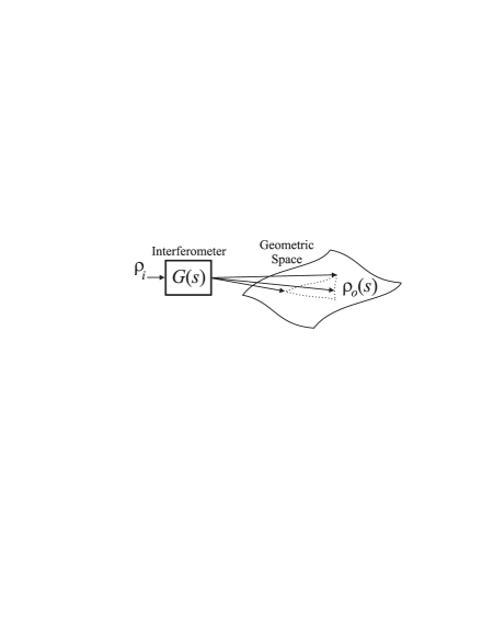
Figure 1: The transformation of the state in the geometric space is depicted diagrammatically. The input state of the interferometer, $\rho_{i}$, is transformed via a parametrized $U(4)$ transformation $G(s)$ to an output state $\rho_{o}(s)$. By adjusting the parameters of the interferometer appropriately, the output state can be made to evolve around a closed path in the geometric space.

As discussed in the introduction, we can view local transformations as gauge transformations that do not alter the entanglement or other nonlocal properties. With local transformations described in terms of this entanglement gauge, we consider two states as equivalent, $\rho^{\prime}\simeq\rho$, if $\rho^{\prime}$ can be obtained from $\rho$ by local operations only. With this equivalence, the output of the interferometer can be identified with the coset space $U(4)/LO$ describing inequivalent states obtained from $\rho$ by nonlocal operations; we refer to $U(4)/LO$ as the geometric space. A general parametrized nonlocal $U(4)$ transformation, then, describes a path $\mathcal{C}$ in this space $U(4)/LO$. If this path is closed, the state will return to the same point $\rho^{\prime}\simeq\rho$ in $U(4)/LO$, equivalent to the initial state to within a local operation. Note that, with this viewpoint, parametrized $U(4)$ transformations in the output space can be implemented without using time $t$ but instead a pseudotime parameter $s$: this parameter, which is a function of the adjustable parameters of the interferometer, can be used for controlled evolution about various paths in the output space San01 ; deG01 .

III Entanglement gauge structure and the non-Abelian geometric phase

In this section, we show how the gauge structure of this space can lead to a non-Abelian geometric phase (NAGP) Wil84 ; Ana88 upon cyclic evolution about a closed path $\mathcal{C}$ in the geometric space $U(4)/LO$. A nonlocal transformation is implemented by adjusting the parameters of the interferometer and is described by the parametrized transformation $G(s)\in U(4)$, $0\leq s\leq s_{0}$. Let the $U(4)$ interferometer initially be set to induce the identity transformation on the input state, so that $G(0)$ is the identity in $U(4)$. The endpoint is chosen such that $G(s_{0})$ closes the path in the geometric space, i.e., $G(s_{0})\in LO$ and thus for any initial state $\rho$ with support in $\mathbb{H}_{(1,1)}$ the final state is

$$\rho^{\prime} =G(s_{0})\rho G(s_{0})^{\dagger}$$

$$\simeq\rho\,.$$ (3)

That is, after cyclic evolution, the transformed state $\rho^{\prime}$ again has support in $\mathbb{H}_{(1,1)}$, and is related to the initial state $\rho$ by a local transformation. The output state of the interferometer will follow a closed path $\mathcal{C}$ in the coset space $U(4)/LO$ parametrized by $s$. Equivalently, we can think of the parametrized $U(4)$ transformation $G(s)$ propagating the subspace $\mathbb{H}_{(1,1)}$ about a closed loop in the Hilbert space $\mathbb{H}_{2}$.

Let $|\psi_{a}(0)\rangle,\ a=1,\ldots,4$ be a basis for $\mathbb{H}_{(1,1)}$ (e.g., the basis of Eq. (II)). We can define a transformed set at each point $s$ along the path as

$$|\psi_{a}(s)\rangle=G(s)|\psi_{a}(0)\rangle\,.$$ (4)

For a closed path $\mathcal{C}$ in the geometric space $U(4)/LO$, the NAGP is given Wil84 ; Ana88 by the Wilson loop

$$K_{\rm NAGP}={\rm P}\exp\{{\rm i}\oint_{\mathcal{C}}\mathcal{A}\}\,,$$ (5)

where the gauge potential $\mathcal{A}$ is given in this basis as a function of the parameter $s$ by

$$\mathcal{A}_{ab}(s) ={\rm i}\langle\psi_{a}(s)|\frac{{\rm d}}{{\rm d}s}|\psi_{b}(s)\rangle\,{\rm d}s$$

$$={\rm i}\langle\psi_{a}(0)|G^{\dagger}(s)\frac{{\rm d}G}{{\rm d}s}|\psi_{b}(0)\rangle\,{\rm d}s\,.$$ (6)

This gauge potential can be expressed in a parameter-independent way as

$$\mathcal{A}_{ab}=\langle\psi_{a}(0)|\Theta_{G}|\psi_{b}(0)\rangle\,,$$ (7)

where the Lie algebra-valued 1-form $\Theta_{G}={\rm i}G^{\dagger}{\rm d}G$ is known as the Maurer-Cartan form. In the following, we will use this Maurer-Cartan form, along with a suitable parametrization of $G$, to derive an explicit expression for the gauge potential $\mathcal{A}$.

III.1 Entanglement gauge transformations

In this formulation, a local unitary transformation $K(s)\in LO$ corresponds to a gauge transformation. Restricted to $\mathbb{H}_{(1,1)}$, it can be viewed as a basis transformation $|\psi_{a}^{\prime}(s)\rangle=K(s)|\psi_{a}(s)\rangle$ with $|\psi_{a}^{\prime}(s)\rangle\in\mathbb{H}_{(1,1)}$. One example of a gauge transformation is a polarization rotation (about any angle) in one spatial mode. Under a gauge transformation, the gauge potential transforms as

$$\mathcal{A}^{\prime}=K^{\dagger}\mathcal{A}K+{\rm i}K^{\dagger}{\rm d}K\,,$$ (8)

and the Wilson loop (5) transforms covariantly Wil84 .

For the special case when $G(s)=K(s)\in LO$, the gauge potential corresponds to a pure gauge. In this situation, $K$ restricted to $\mathbb{H}_{(1,1)}$ satisfies

$${\rm d}(K^{\dagger}{\rm d}K) ={\rm d}K^{\dagger}\wedge{\rm d}K$$

$$={\rm d}K^{\dagger}\wedge KK^{\dagger}{\rm d}K$$

$$={\rm d}K^{\dagger}K\wedge K^{\dagger}{\rm d}K$$

$$=-(K^{\dagger}{\rm d}K)\wedge K^{\dagger}{\rm d}K$$

$$=0\,,$$ (9)

where the penultimate line follows from ${\rm d}(KK^{\dagger})=0$ and the last line is a consequence of the antisymmetry of the wedge product. Hence, $K^{\dagger}{\rm d}K$ is a closed 1-form and therefore on a topologically contractible path is exact. A pure gauge thus does not contribute to the NAGP. As explained in Wil84 , for a general $U(4)$ transformation $G(s)$, it is precisely the (nontrivial) projection of $G^{\dagger}{\rm d}G$ in Eq. (7) onto the subspace $\mathbb{H}_{(1,1)}$ that can induce a nontrivial gauge field $\mathcal{A}_{ab}$. This situation occurs only if nonlocal operations are used.

III.2 Decomposition of group elements

In order to calculate the NAGP acquired by a state $\rho$ undergoing cyclic evolution in $U(4)/LO$, we first construct a decomposition of $U(4)$ into gauge transformations and complementary nonlocal transformations on the coset space $U(4)/LO$. Then, with a suitable parametrization, we derive an expression for the gauge potential $\mathcal{A}$. We begin by decomposing the group $U(4)$ in such a way as to define a simple parametrization for the coset space $U(4)/LO$.

Let $\mathfrak{k}=u(2)^{a}\times u(2)^{b}$ be the set of operators (Hamiltonians) that generate local operations, i.e., the Lie algebra of $LO$. A basis for $\mathfrak{k}$ is given by

$$J_{ax} =\frac{1}{2}(a_{H}^{\dagger}a_{V}+a_{V}^{\dagger}a_{H})\,, \ J_{bx} =\frac{1}{2}(b_{H}^{\dagger}b_{V}+b_{V}^{\dagger}b_{H})\,,$$

$$J_{ay} =\frac{1}{2{\rm i}}(a_{H}^{\dagger}a_{V}-a_{V}^{\dagger}a_{H})\,, J_{by} =\frac{1}{2{\rm i}}(b_{H}^{\dagger}b_{V}-b_{V}^{\dagger}b_{H})\,,$$

$$J_{az} =\frac{1}{2}(a_{H}^{\dagger}a_{H}-a_{V}^{\dagger}a_{V})\,, J_{bz} =\frac{1}{2}(b_{H}^{\dagger}b_{H}-b_{V}^{\dagger}b_{V})\,,$$

$$J_{a0} =\frac{1}{2}(a_{H}^{\dagger}a_{H}+a_{V}^{\dagger}a_{V})\,, J_{b0} =\frac{1}{2}(b_{H}^{\dagger}b_{H}+b_{V}^{\dagger}b_{V})\,.$$ (10)

A complementary set $\mathfrak{p}$ for the Lie algebra $u(4)$ of $U(4)$ is spanned by the eight elements

$$J_{HHx} =\frac{1}{2}(a_{H}^{\dagger}b_{H}+b_{H}^{\dagger}a_{H})\,, J_{HHy} =\frac{1}{2{\rm i}}(a_{H}^{\dagger}b_{H}-b_{H}^{\dagger}a_{H})\,,$$

$$J_{HVx} =\frac{1}{2}(a_{H}^{\dagger}b_{V}+b_{V}^{\dagger}a_{H})\,, J_{HVy} =\frac{1}{2{\rm i}}(a_{H}^{\dagger}b_{V}-b_{V}^{\dagger}a_{H})\,,$$

$$J_{VHx} =\frac{1}{2}(a_{V}^{\dagger}b_{H}+b_{H}^{\dagger}a_{V})\,, J_{VHy} =\frac{1}{2{\rm i}}(a_{V}^{\dagger}b_{H}-b_{H}^{\dagger}a_{V})\,,$$

$$J_{VVx} =\frac{1}{2}(a_{V}^{\dagger}b_{V}+b_{V}^{\dagger}a_{V})\,, J_{VVy} =\frac{1}{2{\rm i}}(a_{V}^{\dagger}b_{V}-b_{V}^{\dagger}a_{V})\,.$$ (11)

Together, $\mathfrak{k}\oplus\mathfrak{p}$ form a basis for the Lie algebra of $U(4)$; thus any group element of $U(4)$ can be expressed as $G=\exp({\rm i}\sum_{i}x_{i}J_{i})$ where $x_{i}$ are real parameters and the sum is running over all 16 generators $J_{i}$ of $\mathfrak{k}\oplus\mathfrak{p}$.

The set $\mathfrak{k}$ is a subalgebra, satisfying $[\mathfrak{k},\mathfrak{k}]\subset\mathfrak{k}$, and the set $\mathfrak{p}$ satisfies $[\mathfrak{k},\mathfrak{p}]\subset\mathfrak{p}$ and $[\mathfrak{p},\mathfrak{p}]\subset\mathfrak{k}$. These properties enable a Cartan decomposition Kna96 of the group $U(4)$, i.e., any element $G\in U(4)$ can be written in the form $G=PK$ with $K\in LO$ and $P$ of the form $\exp({\rm i}\sum_{\mu}x_{\mu}J_{\mu})$ where the sum now runs over the set $\mathfrak{p}$ only.

The group element $P$ can be further simplified via the decomposition

$$P=\bar{K}P_{0}\bar{K}^{\dagger}\,,$$ (12)

where $\bar{K}\in LO$ and

$$P_{0}=\exp({\rm i}x_{H}J_{HHx})\exp({\rm i}x_{V}J_{VVx})\,.$$ (13)

A general proof of this decomposition is given in Appendix A.

Any $\bar{K}$ can be written by using eight real parameters and $P_{0}$ contains two parameters. Thus, because $\mathfrak{p}$ is only eight-dimensional, we can further reduce Eq. (12). Using the Euler parametrization of $SU(2)$, we express $\bar{K}$ as

$$\bar{K}=e^{{\rm i}\alpha_{a}J_{az}}e^{{\rm i}\beta_{a}J_{ay}}e^{{\rm i}\gamma_{a}J_{az}}e^{{\rm i}\delta_{a}J_{a0}}\\ \times e^{{\rm i}\alpha_{b}J_{bz}}e^{{\rm i}\beta_{b}J_{by}}e^{{\rm i}\gamma_{b}J_{bz}}e^{{\rm i}\delta_{b}J_{b0}}\,.$$ (14)

The isotropy group of $x_{V}J_{HHx}+x_{H}J_{VVx}$ is parametrized by $\alpha_{a}-\alpha_{b}$ and $\delta_{a}+\delta_{b}$. Thus, we can define $\alpha_{b}=\delta_{b}=0$ in Eq. (12).

Thus, we can now express any $G\in U(4)$ in the form

$$G=\bar{K}P_{0}K^{\prime}$$ (15)

with $P_{0}$ a two-parameter transformation of the form (13), $\bar{K}$ a six-parameter transformation of the form (14) with $\alpha_{b}=\delta_{b}=0$, and $K^{\prime}=\bar{K}^{\dagger}K\in LO$. Thus, $K$ is an eight-parameter subgroup describing the local (gauge) transformations, and $\bar{K}P_{0}\bar{K}^{-1}$ is a complementary eight-parameter set that generates nonlocal transformations. This decomposition of group elements is a generalization of a method applied by Byrd Byr98 on $SU(3)$.

III.3 Gauge potential and Maurer-Cartan form

Using Eq. (6) we are now able to express the gauge potential in terms of the Maurer-Cartan forms of the group elements $\bar{K},P_{0},K^{\prime}$. With the decomposition $G=\bar{K}P_{0}K^{\prime}$ of Eq. (15), we find

$$\mathcal{A}_{ab} ={\rm i}\langle\psi_{a}(0)|G^{\dagger}{\rm d}G|\psi_{b}(0)\rangle$$

$$={\rm i}\langle\psi_{a}(0)|K^{\prime\dagger}P_{0}^{\dagger}\bar{K}^{\dagger}{\rm d}(\bar{K}P_{0}K^{\prime})|\psi_{b}(0)\rangle$$

$$={\rm i}\langle\psi_{a}(0)|(K^{\prime\dagger}P_{0}^{\dagger})(\bar{K}^{\dagger}{\rm d}\bar{K})(P_{0}K^{\prime})$$

$$\qquad+K^{\prime\dagger}(P_{0}^{\dagger}{\rm d}P_{0})K^{\prime}+K^{\prime\dagger}{\rm d}K^{\prime}|\psi_{b}(0)\rangle$$ (16)

$$=\langle\psi_{a}(0)|K^{\prime\dagger}P_{0}^{\dagger}\Theta_{\bar{K}}P_{0}K^{\prime}$$

$$\qquad+K^{\prime\dagger}\Theta_{P_{0}}K^{\prime}+\Theta_{K^{\prime}}|\psi_{b}(0)\rangle\,.$$

This expression can be greatly simplified as follows. The term containing $\Theta_{K^{\prime}}$ describes a pure gauge; it therefore does not contribute to the NAGP as shown by Eq. (9). The Maurer-Cartan form of $P_{0}$ can easily be calculated from Eq. (13) and is given by

$$\Theta_{P_{0}}=-({\rm d}x_{H})J_{HHx}-({\rm d}x_{V})J_{VVx}\,.$$ (17)

This operator, which mixes the components of the two spatial modes $a$ and $b$, maps the subspace $\mathbb{H}_{(1,1)}$ into its complement. Therefore, because $K^{\prime}|\psi_{b}(0)\rangle$ is an element of $\mathbb{H}_{(1,1)}$, we find that

$$\langle\psi_{a}(0)|K^{\prime\dagger}\Theta_{P_{0}}K^{\prime}|\psi_{b}(0)\rangle=0\,,\quad\forall\ K^{\prime}\in LO\,,$$ (18)

and thus the contribution of $\Theta_{P_{0}}$ to the gauge potential is zero. As a result, the angles $x_{H}$ and $x_{V}$ characterizing the nonlocal operation $P_{0}$ only enter the gauge potential as parameters, and there is no need to integrate over them ($\mathcal{A}$ does not contain ${\rm d}x_{H}$ or ${\rm d}x_{V}$).

The only nontrivial contribution to $\mathcal{A}$ is given by the term containing $\Theta_{\bar{K}}$. In this expression, $K^{\prime}$ only enters as a gauge transformation, and we can fix the gauge by setting $K^{\prime}$ equal to the identity. We call this choice of gauge the entanglement gauge. Thus, $G=\bar{K}P_{0}$ and the final form of the gauge potential is

$$\mathcal{A}_{ab}=\langle\psi_{a}(0)|P_{0}^{\dagger}\Theta_{\bar{K}}P_{0}|\psi_{b}(0)\rangle\,.$$ (19)

Using the Euler decomposition (14) and with $\alpha_{b}=\delta_{b}=0$, we explicitly find

$$\Theta_{\bar{K}}=-(\cos(\beta_{a}){\rm d}\alpha_{a}+{\rm d}\gamma_{a})J_{az}-({\rm d}\gamma_{b})J_{bz}\\ -(\cos(\gamma_{a})\sin(\beta_{a}){\rm d}\alpha_{a}-\sin(\gamma_{a}){\rm d}\beta_{a})J_{ax}\\ -(\cos(\gamma_{b})\sin(\beta_{b}){\rm d}\alpha_{b}-\sin(\gamma_{b}){\rm d}\beta_{b})J_{bx}\\ -(\sin(\gamma_{a})\sin(\beta_{a}){\rm d}\alpha_{a}+\cos(\gamma_{a}){\rm d}\beta_{a})J_{ay}\\ -(\sin(\gamma_{b})\sin(\beta_{b}){\rm d}\alpha_{b}+\cos(\gamma_{b}){\rm d}\beta_{b})J_{by}\\ -({\rm d}\delta_{a})J_{a0}\,.$$ (20)

This explicit expression allows us to calculate the gauge potential $\mathcal{A}_{ab}$ for any path in $U(4)/LO$.

IV Realizing a non-Abelian geometric phase in quantum interferometry

With a parametrization of the coset space $U(4)/LO$ and an explicit expression for the gauge potential in terms of this parametrization, we can now calculate the NAGP acquired by evolution of a state $\rho$ with support in $\mathbb{H}_{(1,1)}$ about a closed path $\mathcal{C}$ in the geometric space $U(4)/LO$ by a parametrized transformation $G(s)\in U(4)$.

IV.1 Parametrized transformations

In order to realize the evolution of a state $\rho$ along a path in $U(4)/LO$, we must construct an interferometer that evolves $\rho$ as $G(s)\rho G(s)^{\dagger}$ for some $G(s)\in U(4)$. Here, $s$ is a pseudotime describing the evolution, and is an adjustable parameter of the interferometer.

We will realize a closed path $\mathcal{C}$ in the geometric space as a sequence of transformations in one-parameter subgroups of $U(4)$. We show in Appendix B that any one-parameter subgroup $U(s)$ of $U(4)$ can be realized in an optical interferometer using variable phase shifts and other fixed linear optical elements. We give examples below where the number of optical elements is kept very small.

Let $\{G_{k}(s_{k});k=1,2,3\}$ be three one-parameter $U(4)$ transformations that perform evolution about a closed path $\mathcal{C}$, with $s_{k}\in\mathbb{R}$ the parameter for each path. The interferometer is constructed to perform the parametrized operation

$$G(s_{1},s_{2},s_{3})=G_{3}(s_{3})G_{2}(s_{2})G_{1}(s_{1})\,,$$ (21)

which can be used to implement cyclic evolution as follows. Initially, all parameters are set equal to zero, and the output state is the initial state $\rho^{(1)}$ in $U(4)/LO$. Parameter $s_{1}$ is made to increase from $0$ to some fixed value $s_{1}^{0}$, resulting in the output state $\rho^{(2)}=G_{1}(s_{1}^{0})\rho^{(1)}G_{1}(s_{1}^{0})^{-1}$. Following this first step, $s_{2}$ is increased from $0$ to $s_{2}^{0}$ yielding the state $\rho^{(3)}$; following that, $s_{3}$ is increased from $0$ to $s_{3}^{0}$ yielding $\rho^{(4)}$. The condition for closure is satisfied if the transformations and parameters are chosen such that

$$G_{3}(s_{3}^{0})G_{2}(s_{2}^{0})G_{1}(s_{1}^{0})\in LO\,,$$ (22)

and thus $\rho^{(4)}\simeq\rho^{(1)}$. The cyclic evolution transports the state about the path $\rho^{(1)}\to\rho^{(2)}\to\rho^{(3)}\to\rho^{(4)}$, where $\rho^{(4)}\simeq\rho^{(1)}$ are both states with support in $\mathbb{H}_{(1,1)}$.

Using our parametrization of elements in $U(4)$ as given in Sec. III.2, we explicitly calculate the NAGP acquired via evolution about such a path. To identify closed paths, we note that $P_{0}(x_{H},x_{V})$ of Eq. (13) only maps $\mathbb{H}_{(1,1)}$ onto itself if $x_{H}=m\pi$ and $x_{V}=n\pi$, for $m,n$ integers that are either both even or both odd. These two conditions identify endpoints for a closed path on $U(4)/LO$.

We now give an explicit construction for evolution about a closed path. Define $G_{1}(s_{1})$ to be

$$G_{1}(s_{1}) =\exp\bigl{(}{\rm i}s_{1}(\cos^{2}\theta J_{HHx}+\sin^{2}\theta J_{VVx})\bigr{)}$$

$$=P_{0}(s_{1}\cos^{2}\theta,s_{1}\sin^{2}\theta)\,,$$ (23)

where $\theta\in[0,\pi/2]$. This transformation, realized using two parametrized polarizing beamsplitters, is inherently nonlocal and evolves any state with support in $\mathbb{H}_{(1,1)}$ to a state with support not entirely within this subspace. The second transformation $G_{2}(s_{2})$ is defined to be

$$G_{2}(s_{2})=\bar{K}(s_{2})\,,$$ (24)

where $\bar{K}(s_{2})$ is an arbitrary one-parameter subgroup of $LO$ such that $\bar{K}(0)$ is the identity. This transformation is implemented using polarization rotators and phase shifters in each mode. Finally, the transformation $G_{3}(s_{3})$ is defined to be

$$G_{3}(s_{3})=\bar{K}P_{0}(s_{3}\cos^{2}\phi,s_{3}\sin^{2}\phi)\bar{K}^{\dagger}\,,$$ (25)

with $\bar{K}=\bar{K}(s_{2}^{0})$, $\phi\in[0,\pi/2]$ and $s_{3}^{0}$ is chosen such that

$$s_{1}^{0}\cos^{2}\theta+s_{3}^{0}\cos^{2}\phi=m\pi\,,$$ (26)

$$s_{1}^{0}\sin^{2}\theta+s_{3}^{0}\sin^{2}\phi=n\pi\,,$$ (27)

for some integers $m,n$ (either both even or both odd). This final transformation is implemented using a combination of polarization rotators and phase shifters (to realize $\bar{K}$ and $\bar{K}^{-1}$) along with two parametrized polarizing beamsplitters (to realize $P_{0}$). With these conditions, the $G_{k}(s_{k})$ satisfy

$$G_{3}(s_{3}^{0})G_{2}(s_{2}^{0})G_{1}(s_{1}^{0})=\bar{K}P_{0}(m\pi,n\pi)\in LO\,.$$ (28)

The gauge potential is zero on paths 1 and 3 because $\mathcal{A}$ does not contain ${\rm d}x_{H}$ or ${\rm d}x_{V}$ and all other differentials are zero. The only contribution to the NAGP therefore comes from path 2 on which we find

$$\mathcal{A}_{ab}=\langle\psi_{a}(0)|P^{\dagger}\Theta_{K}P|\psi_{b}(0)\rangle\,,$$ (29)

where $P=P_{0}(s_{1}^{0}\cos^{2}\theta,s_{1}^{0}\sin^{2}\theta)$. Thus, for our calculations, we only require $P_{0}$ and can otherwise ignore the evolution on paths 1 and 3.

Thus, one can use a $U(4)$ interferometer to evolve a state $\rho$ about a closed path in $U(4)/LO$, and calculate the acquired NAGP by Eqs. (5) and (29). The net transformation on the state $\rho$ upon cyclic evolution will consist of a NAGP due to the geometry of the geometric space and a local gauge transformation; thus, it is not possible to measure the NAGP directly. The effects of this geometric phase can be seen, however, by varying the cyclic paths used. In the following we give a specific example of this procedure.

IV.2 An Example

As an explicit example, we choose $G_{1}(s_{1})$ according to Eq. (IV.1) by setting $\theta=\pi/4$ and $s_{1}^{0}=\pi$. Thus,

$$G_{1}(s_{1})=\exp({\rm i}s_{1}(J_{HHx}+J_{VVx})/2)\,,$$ (30)

which corresponds to a (polarisation-independent) beamsplitter with reflectivity $r=\sin^{2}s_{1}$. As discussed above, this parametrized transformation can be constructed using a variable phaseshifter (parametrized by $s$) and fixed linear optics, in this case, in the form of a Mach-Zehnder interferometer.

For the second portion of the transformation, we choose $G_{2}(s_{2})=\bar{K}(s_{2})$ according to the parametrization of Eq. (14) with $s_{2}=2\beta_{a}=2\beta_{b}$ and all other parameters set to zero. Thus,

$$G_{2}(s_{2})=\exp({\rm i}s_{2}(J_{ay}+J_{by})/2)\,,$$ (31)

with some arbitrary endpoint $s_{2}^{0}>0$. This transformation can be implemented using polarization rotation and phase shifts in each arm (local operations). Finally, to complete the cyclic evolution, we choose $G_{3}$ according to Eq. (25) with $\phi=\pi/4$ and $s_{3}^{0}=\pi$ in order to satisfy the closure condition (26); again, this transformation can be performed using a combination of local operations and a polarization-independent beamsplitter. The interferometer that would realize this cyclic evolution is depicted in Fig. 2.

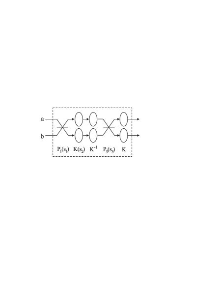
Figure 2: Diagram of an interferometer that would realize a cyclic evolution exhibiting a NAGP. The two spatial modes, $a$ and $b$, have inputs on the left. These spatial modes are combined twice at parametrized beamsplitters, realizing the nonlocal operations $P_{1}(s_{1})=P_{0}(s_{1}/2,s_{1}/2)$ and $P_{3}(s_{3})=P_{0}(s_{3}/2,s_{3}/2)$. Local operations are represented as circles in one spatial mode only, realizing the parametrized operation $K(s_{2})$ and the fixed operations $K$, $K^{-1}$. Note that the cyclic evolution does not occur as the state passes through the interferometer in time; instead, the evolution occurs in pseudotime as the parameters $s_{i}$ are increased from $0$ to $s_{i}^{0}$ in sequence.

Again, we note that only the second path contributes to the NAGP, which we now calculate explicitly. The Maurer-Cartan form for the transformation $\bar{K}(s_{2})$ is

$$\Theta_{\bar{K}}=-\frac{{\rm d}s_{2}}{2}(J_{ay}+J_{by})\,.$$ (32)

Using Eq. (29) and the basis states for $\mathbb{H}_{(1,1)}$,

$$|\psi_{1}(0)\rangle =|HH\rangle\,, |\psi_{2}(0)\rangle =|HV\rangle\,,$$

$$|\psi_{3}(0)\rangle =|VH\rangle\,, |\psi_{4}(0)\rangle =|VV\rangle\,,$$ (33)

we calculate the gauge potential to be

$$\mathcal{A}_{ab}=\frac{{\rm d}s_{2}}{4i}\begin{pmatrix}0&-1&-1&0\\ 1&0&0&-1\\ 1&0&0&-1\\ 0&1&1&0\end{pmatrix}\,.$$ (34)

Integrating along the path gives

$$K_{\rm NAGP}=\exp({\rm i}\int_{0}^{s_{2}^{0}}\mathcal{A})=\begin{pmatrix}C_{+}&-S&-S&C_{-}\\ S&C_{+}&-C_{-}&-S\\ S&-C_{-}&C_{+}&-S\\ C_{-}&S&S&C_{+}\\ \end{pmatrix}$$ (35)

with $S=\frac{1}{2}\sin(s_{2}^{0}/2)$ and $C_{\pm}=\frac{1}{2}(1\pm\cos(s_{2}^{0}/2))$.

With such a setup, it is possible to transform states in $\mathbb{H}_{(1,1)}$ about closed paths, and observe the effects of the geometric phase. The total transformation on the state will be $\bar{K}(s_{2}^{0})P_{0}(\pi,\pi)$, which consists of a combination of a NAGP given by Eq. (35) and a local gauge transformation. The effect of the NAGP can be isolated and observed by varying $s_{2}^{0}$ and evolving a given state about many different paths. In this way, the NAGP can be shown to depend on the geometry of the system, i.e., on the choice of closed path $\mathcal{C}$.

We note that the quantum tomographic techniques of White et al Whi02 have demonstrated that a two-photon state can be completely characterized (with sufficiently many copies of the state or iterations of the experiment). These techniques can be employed in the proposed setup described above to measure the NAGP. Note again that the non-Abelian “phase” described here is a U(4) transformation on a bi-partite density matrix, and thus its effect can readily be observed on an appropriate set of initial states.

It is also possible to realize other cyclic evolutions by choosing different interferometric setups. Another example would be to choose $\theta=0$ and $s_{1}^{0}=\pi$ together with $\phi=0$ and $s_{3}^{0}=\pi$; this choice corresponds to exploying variable beamsplitters which mix only the horizontal (vertical) components for transformations $G_{1}$ ($G_{3}$), respectively. In general, the resulting NAGPs acquired by cyclic evolutions about these different paths will not commute; this non-commutative property is what distinguishes the NAGP from its Abelian counterparts.

V Discussion

Gauge symmetry has proven to be immensely important in theoretical physics, and we have established both a language and a method for applying gauge theory to quantum information theory. The entanglement gauge introduced here establishes an equivalence between actions that differ only by local operations. Nonlocal properties, such as the crucial resource of entanglement, are then regarded as quantities that are invariant under entanglement gauge transformations. Although our focus has been on developing an entanglement gauge for actions on qubits and on pairs of qubits, this analysis could be extended to coupled qudit-qudit systems Bar02 , but of course the group $U(4)$ would need to be replaced by the appropriate larger group.

Gauge theory enables the dynamics to be interpreted geometrically. One way to access information about the geometry by experimental means is via measurements of the geometric phase, and we apply entanglement gauge theory to photonic qubits in interferometry as an experimental means for manifesting and measuring a non-Abelian geometric phase. Although geometric phase experiments for systems with non-Abelian dynamics have been proposed San01 , we have proposed here the first controlled experiment for realizing a non-Abelian geometric phase as opposed to an Abelian geometric phase for a system with non-Abelian dynamics.

It is particularly interesting that this non-Abelian geometric phase is manifested in interferometry, which involves manipulations of the electromagnetic field as the electromagnetic field exhibits a $U(1)$ gauge symmetry. The essential point here in realizing a non-Abelian geometric phase is that the gauge symmetry arises through the equivalence under local operations. We consider sources of entangled qubits, and transform the state to one that is equivalent under local operations with an accumulated non-Abelian geometric phase.

The transformation of the state via linear optics and including an accumulation of a non-Abelian geometric phase requires the state, during its evolution, to leave the space consisting of a single photon in each of the two channels of the interferometer. In leaving this space the evolution includes support from having two photons in one channel, increasing the dimension of the Hilbert space from four to the full ten dimensions of the two-photon irrep of $U(4)$. This evolution out of the four-dimensional Hilbert space is not problematic with respect to the entanglement gauge and the resultant geometry, though, because the interferometer functions as a ‘black box’, as we have carefully described. The key concept here is that the output state is controlled by parameters of the interferometer (which we think of as being controlled by knobs), and the output state evolves along a path in the geometric space as a function of the pseudotime determined by the settings of these knobs. The output state can then be evolved (with evolution parametrized by pseudotime) up to a state equivalent to the initial state up to local operations, with an acquired non-Abelian geometric phase.

We also note that it is possible to map a large class of pseudotime evolutions to a corresponding propagation in real time. This map can be achieved by considering the optical elements (e.g., a phase shifter) as implementing continuous unitary transformations as the photon wavepackets are propagating through the elements. In this sense an optical element that induces a change in pseudotime from $s_{0}$ to $s_{1}$ would correspond to a continuous real-time evolution from $t(s_{0})$ to $t(s_{1})$. By treating each optical element in this way, one arrives at a real- instead of a pseudotime evolution.

For propagation in real time, it is necessary to consider the dynamical evolution of the subspace $\mathbb{H}_{(1,1)}$ introduced in Sec. II. Because the dynamical evolution operator $U_{D}:=\exp(-iHt/\hbar)$ associated with a Hamiltonian $H$ may not commute with the NAGP of Eq. (5), the NAGP becomes difficult to isolate Ana88 . One of the advantages of using optical devices is that this problem can be circumvented; the two photons possess the same energy and the Hamiltonian on the Hilbert space $\mathbb{H}_{2}$ is proportional to the identity operator. Thus, the dynamical evolution $U_{D}$ always commutes with the NAGP and is not relevant.

We have presented the mathematical tools for designing photonic qubit experiments and for determining the resultant non-Abelian geometric phase from a closed-path evolution. A specific example has also been provided in Sec. IV to provide a clear illustration about how such an experiment would be conducted. We observe that three components in the ‘black box’ interferometer are controlled by the pseudotime parameter $s$, and the output state can then be measured by tomographic means: recent tomographic experiments Whi02 have in fact demonstrated the feasibility of such measurements. Generating pure states of entangled photonic qubits, transforming such states via interferometry and measuring the output states via tomography are thus all feasible technologies. Thus, the experimental manifestations of the entanglement gauge are within the reach of current technology.

In summary we have introduced the entanglement gauge and developed the non-Abelian geometric phase as an experimentally realizable manifestation of the entanglement gauge. With the rapid growth in quantum information theory, the entanglement gauge provides a new approach to tackling issues such as analyzing equivalence under local operations, realizing geometric phases in quantum information experiments and connecting operations used in quantum information to principles of differential geometry. Recent proposed applications of geometric phases to fault-tolerant quantum computation Jon00 ; Zan99 suggests that such phases may be useful for quantum information processing. We trust that our entanglement gauge formalism presented here will also prove to be a useful tool for investigations into applications of entanglement, such as entanglement distillation Ben96 , distributed quantum computation Eis00 ; Cir99 , and the ability to perform nonlocal operations using entanglement, local operations and classical communication Eis00 ; Col01 ; Dur01 .

Appendix A Proof of decomposition

The proof of Eq. (13) can be given in a more general form which also applies to a large degree to $U(n)$ in general. To do so we start with a general matrix $M$ of dimension $p\times q$ and consider the exponentation of the $(p+q)\times(p+q)$ matrix,

$$\exp\left[i\left(\begin{array}[]{cc}0&M\\ M^{\dagger}&0\end{array}\right)\right]$$ (36)

One can prove by induction that

$$\left(\begin{array}[]{cc}0&M\\ M^{\dagger}&0\end{array}\right)^{2n}=\left(\begin{array}[]{cc}(MM^{\dagger})^{n}&0\\ 0&(M^{\dagger}M)^{n}\end{array}\right)$$ (37)

which can be used to give a convenient series expansion of the exponential. One now can exploit the singular value decomposition $M=UDU^{\prime\dagger}$, where $U$ and $U^{\prime}$ are unitary matrices of dimension $p\times r$ and $q\times r$, and $r$ the minimum of $p$ and $q$. The matrix $D$ is a real diagonal matrix of dimension $r\times r$. It is then easy to show that $(MM^{\dagger})^{n}=UD^{2n}U^{\dagger}$ as well as $(M^{\dagger}M)^{n}=U^{\prime}D^{2n}U^{\prime\dagger}$. Consequently, the exponential can be written as

$$\exp\left[i\left(\begin{array}[]{cc}0&M\\ M^{\dagger}&0\end{array}\right)\right]\\ =\left(\begin{array}[]{cc}U&0\\ 0&U^{\prime}\end{array}\right)\left(\begin{array}[]{cc}\cos D&i\sin D\\ i\sin D&\cos D\end{array}\right)\left(\begin{array}[]{cc}U^{\dagger}&0\\ 0&U^{\prime\dagger}\end{array}\right)$$ (38)

Restricting to the case $p=q=2$ the exponential corresponds to a general element $P$ in the adjoint representation. In our notation this representation corresponds to the four-dimensional one-photon representation of the generators. The matrices $U$ and $U^{\prime}$ are then general $U(2)$ transformations and just describe the local operations of the subgroup ${\cal K}$. Since $D$ then just contains two independent parameters we find that any nonlocal operation $P$ can be composed of a local operation and a certain nonlocal operation that depends on two parameters only. This result is not in conflict with that of Refs. Cir91 ; mm90 in which three independent parameters are found since in these papers the local operations are restricted to $SU(2)\otimes SU(2)$ transformations only. In our approach we also consider the relative phase shift generated by $J_{a0}-J_{b0}$, which is not an element of $SU(2)\otimes SU(2)$ but of $U(2)\otimes U(2)$, as a local operation.

The explicit form of the middle matrix of the r.h.s. of Eq. (38) just corresponds to the form of $P_{0}$ with $\gamma_{i}$ equal to the diagonal entries of $D$. As this result holds in the adjoint representation and (38) is representation-independent, we infer that the result holds for any representation. This concludes the proof. We remark that this result has a straightforward extension to an $n+n$ decomposition of $U(2n)$.

Appendix B Constructing parametrized $U(4)$ operations

In order to realize a NAGP, it is necessary to perform parametrized $U(4)$ transformations using an optical interferometer. In this appendix, we prove that any one-parameter subgroup $G(s)$ in $U(4)$ can be constructed out of variable phase shifts in each mode and fixed optical elements (such as beamsplitters). This result is a generalization of the Mach-Zehnder inferferometer, where any $SU(2)$ transformation can be implemented using fixed-reflectivity beamsplitters and a variable phase shift in one arm.

A phase shift of one mode (with annihilation operator $c$) is described as a $U(1)$ transformation, generated by an operator of the form $c^{\dagger}c$. Thus, for a $U(4)$ interferometer with four modes, phase shifts in each mode form a subgroup $U(1)\times U(1)\times U(1)\times U(1)\subset U(4)$. Consider a one-parameter (variable) phase shift for the four modes of the $U(4)$ interferometer, generated by an operator of the form

$$D=c_{1}a_{H}^{\dagger}a_{H}+c_{2}a_{V}^{\dagger}a_{V}+c_{3}b_{H}^{\dagger}b_{H}+c_{4}b_{V}^{\dagger}b_{V}\,,$$ (39)

for some real coefficients $c_{i}$. The parametrized transformation

$$S(s)=\exp({\rm i}sD)\,,$$ (40)

thus describes a one-parameter variable phase shift in the four modes, where the relative phase shifts between each of the modes are determined by the coefficients $c_{i}$.

For an arbitrary one-parameter subgroup $G(s)$ of $U(4)$, there exists a fixed matrix $V$ that diagonalizes $G(s)$ for all $s$; i.e.,

$$VG(s)V^{-1}=S(s)\,,$$ (41)

for some $S(s)$ of the form (40). Thus, with the ability to implement the variable phase shift transformation $S(s)$ and the fixed transformation $V$ (and thus also $V^{-1}$), the one-parameter subgroup $G(s)$ can be implemented as $G(s)=V^{-1}S(s)V$.

In addition, it has been shown in deG01 than any (fixed) element in $SU(n)$ can be factorized into a product of $SU(2)$ transformations. With this result, it is possible to construct the required fixed transformations $V$ and $V^{-1}$ out of beamsplitters, phase shifters, and polarization rotations.

- (1) J. Bell, Physics 1, 195 (1964); Rev. Mod. Phys. 38, 447 (1966).
- (2) C. H. Bennett, G. Brassard, C. Crépeau, R. Jozsa, A. Peres and W. K. Wootters, Phys. Rev. Lett. 70, 1895 (1993).
- (3) A. K. Ekert, Phys. Rev. Lett. 67, 661 (1991).
- (4) I. Cirac and N. Gisin, Phys. Lett. A 229, 1 (1997).
- (5) C. A. Fuchs, N. Gisin, R. B. Griffiths, C.-S. Niu and A. Peres, Phys. Rev. A56, 1163 (1997).
- (6) S. L. Braunstein, C. M. Caves, R. Jozsa, N. Linden, S. Popescu and R. Schack, Phys. Rev. Lett. 83, 1054 (1999).
- (7) A. Ekert and R. Jozsa, Philos. Trans. R. Soc., London Ser. A 356, 1769 (1998).
- (8) C. H. Bennett and S. J. Wiesner, Phys. Rev. Lett. 69, 2881 (1992).
- (9) J. Eisert, K. Jacobs, P. Papadopoulos and M. B. Plenio, Phys. Rev. A62, 052317 (2000).
- (10) J. I. Cirac, A. K. Ekert, S. F. Huelga and C. Macchiavello, Phys. Rev. A59, 4249 (1999).
- (11) C. H. Bennett, G. Brassard, S. Popescu, B. Schumacher, J. A. Smolin, and W. K. Wootters, Phys. Rev. Lett. 76, 722 (1996).
- (12) T. Eguchi, P.B. Gilkey and A.J. Hanson, Phys. Rep. 66, 213 (1980).
- (13) M. V. Berry, Proc. Roy. Soc. (Lond.) 392, 45 (1984).
- (14) B. Simon, Phys. Rev. Lett. 51, 2167 (1983); F. Wilczek and A. Shapere, Geometric Phases in Physics, Advanced Series in Mathematical Physics - Vol. 5 (World Scientific, Singapore, 1989).
- (15) I. Fuentes-Guridi, A. Carollo, S. Bose and V. Vedral, Phys. Rev. Lett. 89, 220404 (2002); I. Fuentes-Guridi, S. Bose and V. Vedral, Phys. Rev. Lett. 85, 5018 (2000).
- (16) J. A. Jones, V. Vedral, A. Ekert, and G. Castagnoli, Nature 403, 869 (2000).
- (17) P. Zanardi and M. Rasetti, Phys. Lett. A 264, 94 (1999); J. Pachos, P. Zanardi and M. Rasetti, Phys. Rev. A61, 010305 (2000).
- (18) P. G. Kwiat, K. Mattle, H. Weinfurter, A. Zeilinger, A. V. Sergienko, and Y. Shih, Phys. Rev. Lett. 75, 4337 (1995).
- (19) A. G. White, D. F. V. James, W. Munro and P. G. Kwiat, Phys. Rev. A65, 012301 (2002).
- (20) P. G. Kwiat and R. Y. Chiao, Phys. Rev. Lett. 66, 588 (1991).
- (21) E. Sjöqvist, Phys. Rev. A62, 022109 (2000); B. Hessmo and E. Sjöqvist, Phys. Rev. A62, 062301 (2000).
- (22) E. Sjöqvist, A. K. Pati, A. Ekert, J. S. Anandan, M. Ericsson, D. K. L. Oi, and V. Vedral, Phys. Rev. Lett. 85, 2845 (2000).
- (23) J. I. Cirac and P. Zoller, Phys. Rev. Lett. 74, 4091 (1995).
- (24) S. D. Bartlett, D. A. Rice, B. C. Sanders, J. Daboul, and H. de Guise, Phys. Rev. A63, 042310 (2001).
- (25) N. Lütkenhaus, J. Calsamiglia and K.-A. Suominen, Phys. Rev. A59, 3295 (1999).
- (26) I. L. Chuang and Y. Yamamoto, Phys. Rev. A52, 3489 (1995).
- (27) B. C. Sanders, H. de Guise, S. D. Bartlett and W. Zhang, Phys. Rev. Lett. 86, 369 (2001).
- (28) H. de Guise, B. C. Sanders, S. D. Bartlett and W. Zhang, Czech. J. Phys. 51, 312 (2001).
- (29) F. Wilczek and A. Zee, Phys. Rev. Lett. 52, 2111 (1984).
- (30) J. Anandan, Phys. Lett. A 133, 171 (1988).
- (31) A.W. Knapp, Lie groups beyond an introduction (Birkhauser, Boston, 1996).
- (32) M. Byrd, J. Math. Phys. 39, 6125 (1998); Erratum ibid 41, 1026 (2000).
- (33) S. D. Bartlett, H. de Guise and B. C. Sanders, Phys. Rev. A65, 052316 (2002).
- (34) D. Collins, N. Linden and S. Popescu, Phys. Rev. A64, 032302 (2001).
- (35) W. Dür and J. I. Cirac, Phys. Rev. A64, 012317 (2001).
- (36) W. Dür, G. Vidal, J.I. Cirac, N. Linden, and S. Popescu, Phys. Rev. Lett. 87, 137901 (2001).
- (37) Y. Makhlin, e-print quant-ph/0002045.