Casimir interaction between two concentric cylinders: exact versus semiclassical results

Abstract

The Casimir interaction between two perfectly conducting, infinite, concentric cylinders is computed using a semiclassical approximation that takes into account families of classical periodic orbits that reflect off both cylinders. It is then compared with the exact result obtained by the mode-by-mode summation technique. We analyze the validity of the semiclassical approximation and show that it improves the results obtained through the proximity theorem.

I Introduction

The existence of an attractive force between two uncharged, perfectly conducting parallel plates was predicted by Casimir more than fifty years agoCasimir . Such force has recently been measured at the 15% precision level using cantilevers roberto . A similar force between a conducting plane and a sphere has also been measured with progressively higher precision in the last years using torsion balances Lamoreaux , atomic force microscopes Mohideen , and capacitance bridges chan1 . As described in Ref.chan1 ; chan2 , Casimir forces may be relevant in nanotechnology. The increasing experimental precision revives the interest in the theoretical calculation of Casimir forces and energies for different geometries (see Ref.Bordag for a recent review of experimental and theoretical developments). Only for a few geometries the exact results are known: parallel plates Casimir , self-energy for spheres boyer ; piro ; bowers and cylinders deraad ; nesterenko ; romeo . For the force between a plane and a sphere the exact result is not known, and only an estimation valid when both are close enough is available. This estimation is based on the so called proximity theorem derjaguin . Similar estimations have been recently obtained for the force between two spheres schaden1 . The problems of two concentric spheres saha and two concentric cylinders sahats have also been considered recently. For both cases expressions for the Casimir energy have been obtained using the Abel-Plana formalism. However a detailed numerical calculation and analysis of the results is still missing.

In this paper we compute the Casimir energy for two perfectly conducting and concentric cylinders, using approximate semiclassical methods, and compare the results with those of an exact calculation based on a mode-by-mode summation method. We will show that the semiclassical approximation describes accurately the interaction energy between the cylinders far beyond the range of validity of the proximity theorem.

Let us consider a system of conducting shells $S_{a}$, and denote by $\Lambda$ a suitable set of parameters describing the geometry of the system. For convenience the system is enclosed into a large box, whose boundary $\Sigma$ will eventually be removed to infinity. The Casimir energy can be formally defined as aclaracion

$$E_{c}=E_{0}(\Lambda)-E_{0}(\Lambda_{0})\,\,,$$ (1)

where $E_{0}(\Lambda)$ denotes the zero point energy of the electromagnetic field for the geometry under consideration, and $E_{0}(\Lambda_{0})$ is the one corresponding to the reference vacuum. For semiclassical calculations it will be enough to take the interior of $\Sigma$ without additional conductors as the reference vacuum bd2 . However, for the exact calculation we will use Eq.(1) with $\Lambda_{0}$ describing a system in which the shells are very far away.

In terms of the modes of the electromagnetic field, the Casimir energy can be written as

$$E_{c}={\hbar\over 2}\sum_{p}(w_{p}-\tilde{w}_{p})\,\,\,,$$ (2)

where $w_{p}$ are the eigenfrequencies of the electromagnetic field satisfying perfect conductor boundary conditions on $S_{a}$, and $\tilde{w}_{p}$ are those corresponding to the reference vacuum. The subindex $p$ denotes the set of quantum numbers associated to each eigenfrequency.

For some symmetric systems the Casimir energy can be computed from the sum over modes, Eq.(2). The mode-by-mode summation technique introduced in Ref.piro is based on the use of Cauchy’s theorem to convert the sum over eigenfrequencies into a contour integral, and it turns out to be a very efficient method of calculation in this context.

Alternatively, the Casimir energy can be computed from the knowledge of the density of electromagnetic modes $\rho(E)$ inside $\Sigma$. Of course this is as difficult as computing the sum over modes. However, semiclassical estimates for $\rho(E)$ allow for semiclassical approximations for the Casimir energy schaden1 ; schaden2 . The Casimir energy can be written as

$$E_{c}=\int_{0}^{\infty}\frac{1}{2}\;E\;\Delta\rho(E)\;dE\;,$$ (3)

where

$$\Delta\rho(E)\equiv\sum_{a}\rho_{int,a}+\rho_{ext}-\rho_{vac}\;,$$ (4)

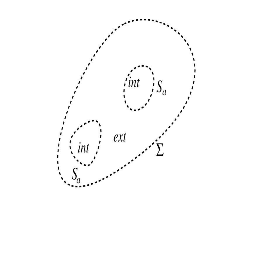
Figure 1: Conducting shells $S_{a}$, not necessarily connected, limiting internal and external regions, with the space cut-off $\Sigma$ limiting the external region.

describes the change in the density of electromagnetic modes inside the box $\Sigma$ when the conducting shells $S_{a}$ are introduced. The spectral density in each region $r=int,ext$ or $vac$ (see Fig.1), $\rho_{r}(E)=\sum_{n}\delta(E-\hbar\omega_{r_{n}})$, is given in terms of a sum on the respective eigenfrequencies $\omega_{r_{n}}$.

Given the Casimir energy, one can compute the forces acting on the shells $S_{a}$ by taking appropriate derivatives with respect to their positions. For the particular case we will consider in this paper, namely two infinite concentric cylinders of radii $a$ and $b$ with $a<b$, it is easy to see using symmetry considerations that the net force on each shell vanishes. However, the pressure is different from zero. For example, the pressure on the inner shell is given by

$$p_{c}=-\frac{1}{2\pi a\ell}\frac{\partial E_{c}}{\partial a}$$ (5)

where $E_{c}$ is the Casimir energy for a length $\ell$.

In Ref.schaden1 ; schaden2 , the Casimir energy for certain systems has been evaluated semiclassically using the fact that in the limit $\hbar\rightarrow 0$, $\Delta\rho(E)$ can be computed as a sum over periodic orbits of a free particle bouncing off the surfaces $S_{a}$. This approximation has been applied to (chaotic) non-symmetric configurations and the contribution of only one isolated periodic trajectory has been considered. This is the case for the force between a plane and a sphere, or for the force between non-concentric spheres. Here we will extend the formalism to symmetric configurations (integrable cavities) in which a whole family of non isolated periodic trajectories contribute significantly in the semiclassical limit.

The paper is organized as follows. In Section II, for those readers not acquainted with semiclassical methods, we present an overview of periodic orbit theory and semiclassical approximations. Section III is devoted to the semiclassical calculation of Casimir interaction between two coaxial cylindrical conductors. In Section IV we compute the exact Casimir energy for the same system, using the mode by mode summation technique. In Section V we present a detailed comparison between the exact, the semiclassical, and the proximity theorem results. Section VI contains the main conclusions of our work.

II Overview of semiclassical methods and Periodic orbit theory: General Formalism

Periodic orbit theory relates oscillations in the quantum level density of a given Hamiltonian to the periodic orbits in the corresponding classical system. It has its origin in the well known decomposition of the spectral density as

$$\rho(E)=\hat{\rho}(E)\,+\rho^{osc}(E);$$ (6)

that has a rigorous meaning only in the semiclassical $(\hbar\rightarrow 0)$ regime for which the scales of variation of $\hat{\rho}(E)$ and $\rho^{osc}(E)$ decouple.

To leading order in $\hbar$ the smooth term $\hat{\rho}(E)$ is the Thomas-Fermi contribution that takes into account the volume of accessible classical phase space at energy $E$. For non relativistic particles confined in cavities with reflecting walls, corrections to $\hat{\rho}(E)$ of higher order in $\hbar$ were first given by Weyl w . Later Balian and Bloch bb1 derived the generalized Weyl formula for cavities with arbitrary smooth convex boundaries and for general classes of boundary conditions. We refer the reader to the book of Baltes and Hilf bal for many details and examples on the Weyl’s expansion.

The deviations from the smooth behavior are given by the oscillating contribution $\rho^{osc}(E)$, which might be written as a sum over classical periodic orbits. The foundations of periodic orbit theory (POT) are closely related to the semiclassical quantization of integrable systems introduced by Bohr and Sommerfeld. Using a multiple reflection expansion for the time independent Green function and employing the principle of stationary phase, Balian and Bloch bb2 derived in 1972 a trace formula for cavities with ideal reflecting walls giving explicit results for spherical cavities. Later Berry and Tabor bt obtained exactly the same formula for integrable cavities using the torus quantization rule and the Poisson summation formula to express the spectral density $\rho(E)$ as a multiple integral and evaluating the integrals by the saddle point method.

The Bohr-Sommerfeld quantization rule fails for quantum Hamiltonian systems whose classical counterpart displays chaotic motion. In 1971 Guztwiller presented his famous trace formula (see Ref. gutz for a review) obtained from Feynman’s path integrals and based on the semiclassical expansion for the single particle propagator. The trace formula obtained by Gutzwiller is only applicable if all the involved periodic orbits are isolated in phase space, being for this reason particularly successful in its applications to chaotic systems. Nevertheless it fails for systems which have degenerate families of non-isolated periodic orbits, such as integrable systems.

POT has been extensively used during the last twenty years to obtain semiclassical estimates for energy spectra of quantum (many-body) systems like atoms and nuclei, with vast applications in nuclear and atomic physics. More recently in condensed matter physics, several transport properties of mesoscopic systems like metal clusters, metallic grains, quantum dots and microstructures have been studied employing the semiclassical tools brack .

In recent works the semiclassical Gutzwiller trace formula was exploited to evaluate the leading order Casimir energy for some “chaotic” configurations of pair of conductors, like two conducting spheres separated a small distance apart or an open shell and a sphere schaden1 ; schaden2 . Although the authors of these works comment on the impossibility to employ Gutzwiller method to evaluate the Casimir energy when non-isolated periodic orbits are present, they did not discuss the possible use of the Balian-Bloch (BB) or Berry-Tabor (BT) trace formulae. As we will show below, they can be properly adapted to evaluate the Casimir effect for integrable configurations of conductors (i.e. spherical shells, cylinders, parallel plates, etc.)

Our approach will be to employ a modified version of the BT trace formula bt , that provides the appropriate path to evaluate semiclassically the Casimir effect for the case of two coaxial cylindrical conductors.

We should also mention that Balian and Duplantierbd obtained the distribution of electromagnetic modes inside a conducting cavity using a multiple scattering expansion for the electromagnetic Green functions, that leads to a decomposition of the spectral density in a smooth and an oscillatory term that can be written as a sum over closed polygons. In a subsequent work they tested the convergence of their method evaluating the Casimir energy for a perfectly conducting sphere bd2 .

$\rho^{osc}$ will turn to be the main ingredient in the semiclassical evaluation of the Casimir energy Eq. (3) and can be written, to leading order in $\hbar$, as a sum gutz

$$\rho^{osc}(E)=\frac{1}{\hbar^{\nu}}\sum_{t}\;A_{t}(E)\;\sin(S_{t}(E)/\hbar\;+\mu_{t})\;,$$ (7)

running over periodic orbits labeled by $t$, where $S_{t}$ is the classical action of the periodic orbit $t$ whose period is $T=dS_{t}/dE$. For photons of energy $E$, the dispersion relation is $E=p\;c$, being $p$ the momentum and $c$ the velocity of light. The classical action along a periodic orbit $t$ is then

$$S_{t}(E)=\oint{\bf p}.\;d{\bf q}=p\;L_{t}=\frac{E}{c}\;L_{t}\;,$$ (8)

with $L_{t}$ the length of the periodic orbit.

The phase $\mu_{t}$ is the so-called Maslov index that counts the number of caustics along the periodic orbit. One should distinguish between Dirichlet and Neumann boundary conditions. For Dirichlet boundary conditions, an additional phase $\pi$ should be taken into account in $\mu_{t}$ for each bounce of the trajectory on the walls of the cavity.

The exponent $\nu$ and the amplitudes $A_{t}$ depend on the type of periodic orbit. For integrable systems with $d$ degrees of freedom, the periodic orbits are non-isolated and form $(d-1)$-parameter families, with the resulting exponent $\nu=(d\;+1)/2$. In chaotic systems the orbits are isolated and their contribution is semiclassicaly smaller with $\nu=1$, irrespective of the dimensionality.

III Semiclassical results for two coaxial cylindrical conductors

We consider two infinite and concentric cylindrical conducting shells $C_{1}$ and $C_{2}$, of radii $a$ and $b$ (with $a<b$). Let us call $\rho_{12}$ the spectral density for photons confined in the region between $C_{1}$ and $C_{2}$ and $\rho^{osc}_{12}$ the corresponding leading order oscillating contribution. To obtain $\rho^{osc}_{12}$ one can derive à la BT a trace formula for photons inside the conducting shells, starting from the Hamiltonian $H=E=p\;c$, employing Poisson summation formula and using the torus quantization rule majo . However we find it easier to proceed in two steps. Firstly, if one knows the oscillating contribution $\rho^{osc}(E_{m})$ for non-relativistic particles of mass $m$ and energy $E_{m}={p_{m}}^{2}/2m$ confined in a given cavity, the oscillating contribution for photons confined in the same cavity is obtained from $\rho^{osc}(E_{m})$ after replacing $E_{m}\rightarrow p/c$ and $p_{m}/m\rightarrow c$. This is not restricted to the oscillating contribution, and the same replacement could be done in the complete spectral density $\rho$. Secondly, for cavities with axial symmetry, and in particular for the geometry under consideration, the periodic orbits (PO) are contained in planes perpendicular to the $z$ axis (we are considering cylinders of infinite length). Therefore if one knows the oscillating contribution to the spectral density in the bidimensional annular region between two disks, $\rho^{osc}_{\odot}$, it its straightforward to obtainmajo that, for a given length $\ell$,

$$\rho^{osc}_{12}(E=\hbar c\;k)=\frac{\ell}{\hbar\;c\pi}\;\int_{0}^{k}\frac{k}{\sqrt{k^{2}-k_{z}^{2}}}\;\rho^{osc}_{\odot}(\sqrt{k^{2}-k_{z}^{2}})\;dk_{z}\;.$$ (9)

We stress that the above equation is valid for cavities with axial symmetry, but with generic transverse sections.

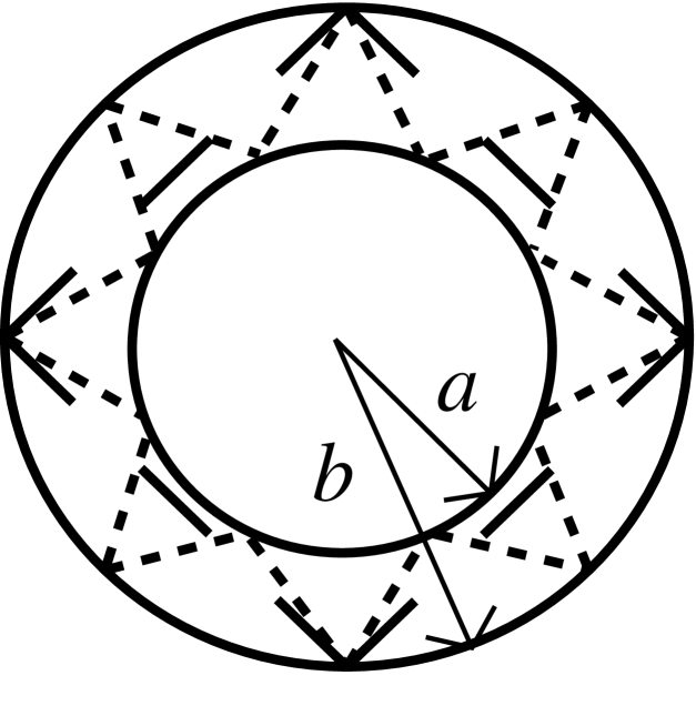
Figure 2: Two periodic orbits in a bidimensional annular region. The type-I orbit $(v=4,w=1)$ does not touch the inner disk (long-dashed line). The type-II orbit $(v=8,w=1)$ hit it (short-dashed line).

The oscillating contribution for non-relativistic particles confined in bidimensional annular regions, $\rho^{osc}_{\odot}(E_{m})$ has been previously derived (see e.g. Richter’s book in Ref.brack and Appendix A). In this configuration there are two types of PO (see Fig. 2): those which do not touch the inner disk (type-I), and those which do hit it (type-II).

The type-I orbits are polygons that may be uniquely labeled by two integers $(v,w)$ where $v$ is the number of vertices (or sides) and $w$ the winding number around the center. For $w=1$ one has ordinary regular polygons, and for $w>1$ star-like polygons, except if $v$ and $w$ are coprimes. In this situation the label $(v,w)=(n\;j,n\;k)$ describes the $n^{th}$ repetition of the primitive orbit with $j$ vertices and winding number $k$. Type-I orbits must fulfill $v\geq\hat{v}(w)\equiv Int[w\pi/\arccos(a/b)]$, that is the minimum value of $v$ depends on $w$ and the ratio $a/b$ between the radii of the inner and outer cylinders, respectively. This is a geometrical restriction due to the fact that $\cos(\pi w/v)>a/b$. The lengths $L_{vw}$ of these orbits are

$$L_{vw}=2\,v\;b\sin(\pi w/v)\;.$$ (10)

Type-II trajectories are labeled by $(v,w)$, where now $w$ is the number of turns around the inner disk in order to come back to the initial point after $v$ bounces on the outer circle of radius $b$. We have the same restriction $v\geq\hat{v}(w)$ as for type-I trajectories and the length is given by

$$\bar{L}_{vw}=2\,v\;b\;\sqrt{\left(1+\;\left(\frac{a}{b}\right)^{2}\;-2\;\frac{a}{b}\;\cos(\pi w/v)\right)}\;.$$ (11)

Following the steps described above, we write $\rho^{osc}_{12}\equiv\rho^{osc}_{12,I}+\rho^{osc}_{12,II}$ as a sum of two terms that take into account the contributions of type-I and type-II PO, respectively. We find (see Appendix A)

$$\rho^{osc}_{12,I}(E) = \sum_{w\geq 1}\;\sum_{v\geq\hat{v}}\frac{\ell}{\pi(\hbar c)^{2}}\;\frac{L_{vw}}{v^{2}}\;E\;\sin\left(\frac{E}{\hbar c}\;L_{vw}\pm\frac{v\;\pi}{2}+\frac{\pi}{2}\right)\;,$$ (12)

$$\rho^{osc}_{12,II}(E) = \sum_{w\geq 0}\;\sum_{v\geq\hat{v}}f_{vw}\;\frac{2\ell}{\pi(\hbar c)^{2}}\frac{b^{2}}{\bar{L}_{vw}}\;A_{vw}\;E\;\sin\left(\frac{E}{\hbar c}\;\bar{L}_{vw}\right)\;.$$ (13)

The $+(-)$ in Eq.(12) corresponds to Dirichlet (Neumann) boundary conditions (bc). On the other hand, there is no additional phase and therefore no difference between Dirichlet and Neumann bc in the type-II contribution, Eq.(13). The coefficient $f_{vw}$ is given by $f_{vw}=2$, except for the self-retracing type-II orbit, that has $w=0$ and $v=2$, for which $f_{20}=1$. In Eq.(13) we have defined

$$A_{vw}\equiv\sqrt{\left(1-\;\frac{a}{b}\;\cos(\pi w/v)\right)\;\left(\frac{a}{b}\;\cos(\pi w/v)-\left(\frac{a}{b}\right)^{2}\right)}\;.$$ (14)

Having obtained the explicit expression for the oscillating contribution to the spectral density in the region between two coaxial cylinders we can use this expression to estimate the semiclassical contribution to the Casimir interaction in that region. For this purpose, we need to rewrite Eq.(4) for the present configuration of conductors. The internal region is now formed by the two conducting shells. We take the outer cylindrical shell $C_{2}$ as the shell that limits the internal and external regions. Therefore we write,

$$\rho_{int}=\rho_{1}+\;\rho_{12}\;,$$ (15)

where $\rho_{1}$ is the density of electromagnetic modes inside the cylindrical shell $C_{1}$. $\rho_{12}$ has been already defined and its oscillating contribution computed in Eqs.(12) and (13).

In order to employ the semiclassical decomposition of the spectral densities in each region $r$, Eq.(6), we derive the smooth contributions $\hat{\rho}_{r}(E)$. Starting from the Weyl expansion for the non-relativistic case w ; bb2 and following again the steps described above, we obtain

$$\hat{\rho}_{r}(E)=\frac{\pi\;E^{2}}{2\;(\hbar\;c\;\pi)^{3}}\;{\cal V}_{r}\;\mp\frac{\pi\;E}{8\;(\hbar\;c\;\pi)^{2}}\;{\cal S}_{r}\;+{\cal O}(1/\hbar)\;,$$ (16)

where ${\cal V}_{r}$ and ${\cal S}_{r}$ are the volume and the surface area of each region $r$. The $-(+)$ sign in the surface term corresponds to Dirichlet (Neumann) bc.

Therefore replacing Eqs.(6), (15) and (16) in Eq.(4) we obtain, to leading order in $\hbar$,

$$\Delta\rho^{sem}(E)=\Delta\hat{\rho}(E)\;+\Delta\rho^{osc}(E)=\rho^{osc}_{1}(E)+\;\rho^{osc}_{12}(E)+\;\rho^{osc}_{ext}(E)-\;\rho^{osc}_{vac}(E)\;,$$ (17)

where the label $sem$ is employed to emphasize the explicit use of the semiclassical decomposition, Eq.(6). The cancellation, to leading order in $\hbar$, of the net smooth contribution $\Delta\hat{\rho}(E)$ is a consequence of the identity ${\cal V}_{1}\;+{\cal V}_{12}\;+{\cal V}_{ext}-{\cal V}_{vac}=0$

For the geometry under study, and when considering the total electromagnetic (e.m.) contribution, it is satisfied that $\Delta\hat{\rho}(E)=0$ to next-to-leading order in $\hbar$. This is due to the opposite sign of the surface term in Eq.(16) for the Dirichlet and Neumann bc.

As already mentioned, in order to compute the Casimir energy Eq.(3) one has to remove to infinity the boundary $\Sigma$ that enclose the reference vacuum. In this limit $\rho^{osc}_{ext}(E)\rightarrow 0$ and $\rho^{osc}_{vac}(E)\rightarrow 0$ since no PO survive in the limit $\Sigma\rightarrow\infty$. Taking this into account and in order to compare the semiclassical results with the exact calculations, we define in analogy to Eq.(3)

$$E^{sem}\equiv\frac{1}{2}\int_{0}^{\infty}E\;\Delta\rho^{sem}(E)\;dE\;=\frac{1}{2}\int_{0}^{\infty}E\ \left(\rho^{osc}_{1}(E)+\;\rho^{osc}_{12}(E)\right)\;dE\equiv E^{osc}_{1}\;+E^{osc}_{12}\;.$$ (18)

It is a well known result that in the case of cylindrical geometries the Casimir energy for the electromagnetic case (e.m.) can be computed as the sum of the Dirichlet and Neumann scalar contributions. Thus, one has

$$E^{sem}=\;E^{osc}_{1}\;+E^{osc}_{12}\;=E^{osc}_{1,D}\;+E^{osc}_{1,N}+\;E^{osc}_{12,D}\;+E^{osc}_{12,N}\;,$$ (19)

where the subscript $D(N)$ stands for Dirichlet (Neumann) bc.

We now turn our attention to $\rho^{osc}_{1}(E)$, the oscillating contribution for the density of modes inside $C_{1}$. We derive $\rho^{osc}_{1}(E)$ adapting the previous result Eq.(12). The PO are the same type-I polygons labeled by two integers $(v,w)$. Being $a$ the radius of $C_{1}$, the length of these orbits is now ${\tilde{L}}_{vw}=2\,v\;a\sin(\pi w/v)$, the shortest one corresponds to the self-retracing diametrical orbit that has $v=2,w=1$. For a cylindrical shell like $C_{1}$, it is satisfied that $v\geq 2w$, that is $\hat{v}=2\;w$. In other words, the cylindrical cavity is the annular one with a vanishing inner radius. Therefore,

$$\rho^{osc}_{1,bc}(E)=\;\sum_{w\geq 1}\;\sum_{v\geq 2w}\;g_{vw}\;\frac{\ell}{2\pi(\hbar c)^{2}}\;\frac{{\tilde{L}}_{vw}}{v^{2}}\;E\;\sin\left(\frac{E}{\hbar c}\;{\tilde{L}}_{vw}\pm\frac{v\;\pi}{2}+\frac{\pi}{2}\right)\;,$$ (20)

where again the $+(-)$ sign corresponds to $bc=D(bc=N)$. The prefactor is $g_{21}=1$ for the self-retracing orbit and $g_{vw}=2$ otherwise.

Taking into account that

$$E^{osc}_{1}=E^{osc}_{1,D}+\;E^{osc}_{1,N}=\;\frac{1}{2}\int_{0}^{\infty}E\left(\rho^{osc}_{1,D}(E)\;+\rho^{osc}_{1,N}(E)\right)dE\;,$$ (21)

we perform the energy integration employing Eq.(20) and an exponential cutoff. It is straightforward to show that

$$\int_{0}^{\infty}E^{2}\sin\left(\frac{E}{\hbar c}\;{\tilde{L}}_{vw}\pm\frac{v\;\pi}{2}+\frac{\pi}{2}\right)\;dE=\lim_{\lambda\rightarrow 0}\int_{0}^{\infty}\exp{(-\lambda\;E)}\;E^{2}\sin\left(\frac{E}{\hbar c}\;{\tilde{L}}_{vw}\pm\frac{v\;\pi}{2}+\frac{\pi}{2}\right)\;dE$$ (22)

$$= \pm 2\;\left(\frac{\hbar\;c}{{\tilde{L}}_{vw}}\right)^{3}\;\sin(\pi\;v/2)\;,$$

and in conclusion

$$E^{osc}_{1}=E^{osc}_{1,D}\;+E^{osc}_{1,N}=\;0\;.$$ (23)

Thus in the semiclassical approximation, the e.m. Casimir energy for an isolated cylinder vanishes. This is also the case to lowest order in the multiple scattering expansion bd2 .

To compute $E^{osc}_{12}=E^{osc}_{12,D}+\;E^{osc}_{12,N}$ we should take into account, in principle, both type-I and type-II PO for each scalar contribution, $D$ or $N$. However, as before, the contributions from type-I PO cancel out and only type-II PO contribute to the semiclassical e.m. Casimir interaction. We compute $E^{osc}_{12}$ noting that $\rho^{osc}_{12,II}$ is the same for Dirichlet and Neumann bc and therefore

$$E^{osc}_{12}=2\;\frac{1}{2}\int_{0}^{\infty}E\;\rho^{osc}_{12,II}(E)\;dE\;.$$ (24)

Replacing $\rho^{osc}_{12,II}$ from Eq.(13) and performing again the energy integration using an exponential cutoff, we obtain the main result of this section. Namely,

$$E^{sem}=\;E^{osc}_{12}=\;-\ell\frac{\hbar\;c}{4\;\pi\;a^{2}}\;\alpha^{1/2}\;\sum_{w\geq 0}\;\sum_{v\geq\hat{v}}f_{vw}\;\frac{1}{v^{4}}\;N(\alpha,v,w)\,\,,$$ (25)

where we have defined $\alpha\equiv b/a$, and

$$N(\alpha,v,w)\;\equiv\frac{\sqrt{\left(\alpha-\;\cos(\pi w/v)\right)\;\left(\alpha\;\cos(\pi w/v)-\;1\right)}}{\left(1\;+\alpha^{2}\;-2\;\alpha\;\cos(\pi w/v)\right)^{2}}\;.$$ (26)

It is interesting to rewrite Eq.(25) by separating the terms with $w=0$ from those with $w\geq 1$. The orbits with $w=0$ and $v\geq 1$ are the diametrical orbit and its repetitions, whose lengths are $\bar{L}_{v0}=2\;v\;(b\;-\;a)$. Therefore we write

$$E^{sem}\equiv E^{sem}_{w=0}\;+E^{sem}_{w\geq 1}=\;E^{sem}_{w=0}-\;\ell\frac{\hbar\;c}{2\;\pi\;a^{2}}\;\alpha^{1/2}\;\sum_{w\geq 1}\;\sum_{v\geq\hat{v}}\;\frac{1}{v^{4}}\;N(\alpha,v,w)\;.$$ (27)

In order to obtain $E^{sem}_{w=0}$, we calculate from Eq.(26)

$$N(\alpha,v,0)=\frac{1}{(\alpha\;-1)^{3}}\;,$$ (28)

and using the fact that $\sum_{v\geq 1}\;v^{-4}=\zeta(4)={\pi^{4}}/{90}$ we finally obtain,

$$E^{sem}_{w=0}=\;-\ell\;\frac{\hbar\;c\;\pi^{3}}{360\;a^{2}}\;\frac{\sqrt{\alpha}}{(\alpha\;-1)^{3}}\;=-\ell\;\frac{\hbar\;c\;\pi^{3}}{360}\;\frac{\sqrt{a\;b}}{(b\;-a)^{3}}\;.$$ (29)

This expression, which is valid for arbitrary values of $\alpha>1$, diverges as $\alpha\rightarrow 1$. One might wonder whether the sum of the contributions with $w\geq 1$ cancels and/or contributes, in any way, to this divergence. To investigate this problem it is interesting to note that, in such a limit, it is possible to derive an analytic expression for the sum of these contributions. Due to the fact that for $\alpha\sim 1$,

$$\hat{v}\equiv Int[w\pi/\arccos(a/b)]\sim\frac{\pi\;w\sqrt{\alpha}}{\sqrt{2\;(\alpha-\;1)}}>>\;w\;,$$ (30)

we can approximate $\cos(\pi w/v)\sim 1\;-{(\pi\;w/v)}^{2}/2$. Thus, from Eq.(26)

$$N(\alpha\sim 1,v,w)=\;\frac{1}{(\alpha\;-1)^{3}}\;\frac{v^{4}-\frac{(\pi\;w)^{4}}{16\;(\alpha-\;1)^{2}}}{\left(v^{2}+\frac{(\pi\;w)^{2}\;\alpha}{(\alpha-\;1)^{2}}\right)^{2}}\;.$$ (31)

Since $\hat{v}>>1$ we can convert the sum $\sum_{v\geq\hat{v}}\;\frac{1}{v^{4}}\;N(\alpha\sim 1,v,w)$ in Eq.(27) into an integral. Performing the integration and summing over $w\geq 1$ we obtain

$$E^{sem}_{w\geq 1}(\alpha\sim 1)=-\;\ell\frac{\hbar\;c}{4\;\pi^{3}\;a^{2}}\frac{\zeta(3)}{\alpha}\;+{\cal O}(\alpha\;-1),$$ (32)

which implies that $E^{sem}_{w\geq 1}$ remains finite as $\alpha\rightarrow 1$. Thus, in this limit the semiclassical result is divergent and completely dominated by the $w=0$ contribution. As we will see later, this dominance extends over a rather large range of values of $\alpha$.

Having shown that for $\alpha\sim 1$ one has $E^{sem}\sim E^{sem}_{w=0}$ it is interesting to compare Eq.(29) with what results from the application of the proximity theorem derjaguin . The Casimir energy between two parallel plates of area $A$ separated a small distance $\delta$ is

$$E_{||}=-\;\frac{\hbar\;c\;\pi^{2}}{720}\frac{A}{\delta^{3}}\,\,.$$ (33)

For the two coaxial cylinders, when $(b\;-a)\ll a\sim b$, the proximity approximation for the Casimir energy, $E_{P}$, is obtained taking $\delta\;=(b\;-a)$ and $A\rightarrow 2\;\pi\ell\;a\sim 2\;\pi\;\ell b\;$ in Eq.(33). The result is

$$E_{P}=\left\{\begin{array}[]{ll}-\ell\;\frac{\hbar\;c\;\pi^{3}}{360}\;\frac{a}{(b\;-a)^{3}}&\mbox{for $\;A=2\;\pi\ell\;a$ ,}\\ -\ell\;\frac{\hbar\;c\;\pi^{3}}{360}\;\frac{a\;\alpha}{(\alpha\;-1)^{3}}&\mbox{for $\;A=2\;\pi\ell\;b.$}\end{array}\right.$$ (34)

The proximity theorem does not suggest any particular choice for the area A. This is irrelevant in the limit $\alpha\sim 1$.

The semiclassical result Eq.(29) can be interpreted as a proximity approximation with a given choice for the area: the geometric mean between the areas of both cylinders. Although it has been shown that to compute a proximity force for a “chaotic” geometry, the geometric mean radius should be taken blocki , such demonstration does not apply to the present case. However, the semiclassical approximation provides a justification for it. As we will see in Section V, this choice reproduces the exact pressure with an error less than $10\%$ for $1<\alpha<4$, improving the proximity result beyond its expected range of validity.

IV Exact Casimir energy

In this section we will compute the exact Casimir energy for the coaxial cylinders using the mode by mode summation method of Ref.piro .

The zero point energy in Eq.(2) is ill defined, because both series are divergent. In order to define it properly we introduce a cutoff function as follows

$$E_{ex}(\sigma)={\hbar\over 2}\sum_{p}(e^{-\sigma w_{p}}w_{p}-e^{-\sigma\tilde{w}_{p}}\tilde{w}_{p})\;.$$ (35)

The exact Casimir energy $E_{ex}$ is the limit of $E_{ex}(\sigma)$ as $\sigma\rightarrow 0$. For simplicity we choose an exponential cutoff, although the explicit form is not relevant. In our definition we take $w_{p}$ as the eigenfrequencies of the electromagnetic field satisfying perfect conductor boundary conditions at $r=a,r=b$ and $r=R$, and $\tilde{w}_{p}$ are those corresponding to the boundary conditions at $r=R_{1},r=R_{2}$ and $r=R$, in the limit $R>R_{2}>R_{1}\gg a>b$. $R_{1},R_{2}$ and $R$ are the parameters that define the reference vacuum (see Eq. (1)). $R$ corresponds in this case to the radius of the surface $\Sigma$ in Fig.1.

In cylindrical coordinates, the eigenfunctions are of the form

$$h_{nk_{z}}(t,r,\theta,z)=e^{(-iw_{nk_{z}}t+ik_{z}z+in\theta)}R_{n}(\lambda r)\;,$$ (36)

where the function $R_{n}$ is a combination of Bessel functions satisfying the perfect conductor boundary conditions. These boundary conditions define the possible values of the constant $\lambda$. The eigenfrequencies are $w_{nk_{z}}=c\sqrt{k_{z}^{2}+\lambda^{2}}$.

The frequencies of the TE modes are defined by the following relations:

$$J_{n}(\lambda a)=0\,\,\,\,\,\,\,\,\,\,\,\,\,\,\,\,\,\,\,\,r<a$$

$$J_{n}(\lambda a)N_{n}(\lambda b)-J_{n}(\lambda b)N_{n}(\lambda a)=0\,\,\,\,\,\,\,\,a<r<b$$

$$J_{n}(\lambda b)N_{n}(\lambda R)-J_{n}(\lambda R)N_{n}(\lambda b)=0\,\,\,\,\,\,\,\,b<r<R\;.$$ (37)

For later use we introduce the notation $F_{n}^{TE}$ for the product of these three relations

$$F_{n}^{TE}(z,a,b,R)=J_{n}(za)[J_{n}(za)N_{n}(zb)-J_{n}(zb)N_{n}(za)][J_{n}(zb)N_{n}(zR)-J_{n}(zR)N_{n}(zb)]\;.$$ (38)

The frequencies of the TM modes involve derivatives of the Bessel functions:

$$J^{\prime}_{n}(\lambda_{nm}a)=0\,\,\,\,\,\,\,\,\,\,\,\,\,\,\,\,\,\,\,\,r<a$$

$$J^{\prime}_{n}(\lambda_{nm}a)N^{\prime}_{n}(\lambda_{nm}b)-J^{\prime}_{n}(\lambda_{nm}b)N^{\prime}_{n}(\lambda_{nm}a)=0\,\,\,\,\,\,\,\,a<r<b$$

$$J^{\prime}_{n}(\lambda_{nm}b)N^{\prime}_{n}(\lambda_{nm}R)-J^{\prime}_{n}(\lambda_{nm}R)N^{\prime}_{n}(\lambda_{nm}b)=0\,\,\,\,\,\,\,\,b<r<R\;.$$ (39)

As before, we introduce the notation

$$F_{n}^{TM}(z,a,b,R)=J^{\prime}_{n}(za)[J^{\prime}_{n}(za)N^{\prime}_{n}(zb)-J^{\prime}_{n}(zb)N^{\prime}_{n}(za)][J^{\prime}_{n}(zb)N^{\prime}_{n}(zR)-J^{\prime}_{n}(zR)N^{\prime}_{n}(zb)]\;.$$ (40)

The set of quantum numbers $p$ in Eq. (35) is given by $(n,m,k_{z})$, where $m$ denotes the different solutions $\lambda_{nm}$ of both $F_{n}^{TE}(z,a,b,R)=0$ and $F_{n}^{TM}(z,a,b,R)=0$ . As we are considering infinite cylinders, we can replace the sum over $k_{z}$ by an integral. The result for the Casimir energy for a length $\ell$ is

$$E_{ex}(\sigma)={\ell\hbar c\over 2}\int_{-\infty}^{\infty}{dk_{z}\over 2\pi}\sum_{n,m}\left(\sqrt{k_{z}^{2}+\lambda_{nm}^{2}}e^{-\sigma c\sqrt{k_{z}^{2}+\lambda_{nm}^{2}}}-\sqrt{k_{z}^{2}+\tilde{\lambda}_{nm}^{2}}e^{-\sigma c\sqrt{k_{z}^{2}+\tilde{\lambda}_{nm}^{2}}}\right)\;,$$ (41)

where we have denoted with $\tilde{\lambda}_{nm}$ the solutions of the equations $F_{n}^{TE}(z,R_{1},R_{2},R)=0$ and $F_{n}^{TM}(z,R_{1},R_{2},R)=0$.

Using Cauchy’s theorem it follows that

$${1\over 2\pi i}\int_{C}\,dz\;z\;e^{-\sigma z}{d\over dz}\ln f(z)=\sum_{i}x_{i}\;e^{-\sigma x_{i}}\;,$$ (42)

where $f(z)$ is an analytic function within the closed contour $C$, with simple zeros at $x_{1},x_{2},...,$ within $C$. Following Refs. piro ; bowers , we use this result to replace the sum over $m$ in Eq.(41) by a contour integral

$$E_{c}(\sigma)={\ell\hbar c\over 4\pi i}\int_{-\infty}^{\infty}{dk_{z}\over 2\pi}\sum_{n}\int_{C}dz\sqrt{k_{z}^{2}+z^{2}}e^{-\sigma c\sqrt{k_{z}^{2}+z^{2}}}{d\over dz}\ln F^{EM}_{n\ 2cyl}(z,a,b)\;,$$ (43)

where

$$F^{EM}_{n\ 2cyl}(z,a,b)=\lim_{R_{1},R_{2},R\rightarrow\infty}{F_{n}^{TE}(z,a,b,R)F_{n}^{TM}(z,a,b,R)\over F_{n}^{TE}(z,R_{1},R_{2},R)F_{n}^{TM}(z,R_{1},R_{2},R)}\;.$$ (44)

It proves to be convenient to compute the difference between the energy of the system of two concentric cylinders and the energy of two isolated cylinders of radii $a$ and $b$

$$E_{12}(\sigma)=E_{c}(\sigma)-E_{1}(\sigma,a)-E_{1}(\sigma,b)\;.$$ (45)

The energy of isolated cylinders has been computed previously using other regularizations deraad ; nesterenko . The formal expression with the cutoff can be obtained adapting the two cylinders case above. It is given by

$$E_{1}(\sigma,a)={\ell\hbar c\over 4\pi i}\int_{-\infty}^{\infty}{dk_{z}\over 2\pi}\sum_{n}\int_{C}dz\sqrt{k_{z}^{2}+z^{2}}e^{-\sigma c\sqrt{k_{z}^{2}+z^{2}}}{d\over dz}\ln F^{EM}_{n\ 1cyl}(z,a)\;,$$ (46)

where

$$F^{EM}_{n\ 1cyl}(z,a)=\lim_{R_{1},R\rightarrow\infty}{F_{n}^{(1)TE}(z,a,R)F_{n}^{(1)TM}(z,a,R)\over F_{n}^{(1)TE}(z,R_{1},R)F_{n}^{(1)TM}(z,R_{1},R)}$$ (47)

and

$$F_{n}^{(1)TE}(z,a,R) = J_{n}(za)[J_{n}(za)N_{n}(zR)-J_{n}(zR)N_{n}(za)]$$

$$F_{n}^{(1)TM}(z,a,R) = J^{\prime}_{n}(za)[J^{\prime}_{n}(za)N^{\prime}_{n}(zR)-J^{\prime}_{n}(zR)N^{\prime}_{n}(za)]\;.$$ (48)

Therefore, the explicit form for $E_{12}$ is

$$E_{12}(\sigma)={\ell\hbar c\over 4\pi i}\int_{-\infty}^{\infty}{dk_{z}\over 2\pi}\sum_{n}\int_{C}dz\sqrt{k_{z}^{2}+z^{2}}e^{-\sigma c\sqrt{k_{z}^{2}+z^{2}}}{d\over dz}\ln F_{n\ 12}(z,a,b)\;,$$ (49)

where

$$F_{n\ 12}(z,a,b)={F^{EM}_{n\ 2cyl}(z,a,b)\over F^{EM}_{n\ 1cyl}(z,a)F^{EM}_{n\ 1cyl}(z,b)}\;.$$ (50)

To proceed we must choose a contour for the integration in the complex plane. In order to compute $E_{ex}(\sigma),E_{1}(\sigma,a)$ and $E_{1}(\sigma,b)$ separately, an adequate contour is bowers a circular segment $C_{\Gamma}$ and two straight line segments forming an angle $\phi$ and $\pi-\phi$ with respect to the imaginary axis (see Fig. 3). The nonzero angle $\phi$ is needed to show that the contribution of $C_{\Gamma}$ vanishes in the limit $\Gamma\rightarrow\infty$ when $\sigma>0$. For the rest of the contour, it can be shown that the divergences in $E_{ex}(\sigma)$ are cancelled out by those of $E_{1}(\sigma,a)$ and $E_{1}(\sigma,b)$. Therefore in order to compute $E_{12}(\sigma)$ we can set $\phi=0$ and $\sigma=0$. The contour integral reduces to an integral on the imaginary axis. We find

$$E_{12}=-{\ell\hbar c\over 2\pi a^{2}}\int_{-\infty}^{\infty}{dk_{z}\over 2\pi}\sum_{n}Im\left\{\int_{0}^{\infty}dy\sqrt{k_{z}^{2}-y^{2}}{d\over dy}\ln F_{n\ 12}(iy,1,\alpha)\right\}\;,$$ (51)

where we have used that $F_{n\ 12}(iy/a,a,b)=F_{n\ 12}(iy,1,\alpha)$.

Using the asymptotic expansions of Bessel functions we obtain, on the imaginary axis aclaracion2

$$F^{EM}_{n\ 2cyl}(iy,1,\alpha) = 16\alpha^{2}y^{4}I_{n}(y)I^{\prime}_{n}(y)[I_{n}(y)K_{n}(\alpha y)-I_{n}(\alpha y)K_{n}(y)]$$ (52)

$$[I^{\prime}_{n}(y)K^{\prime}_{n}(\alpha y)-I^{\prime}_{n}(\alpha y)K^{\prime}_{n}(y)]K_{n}(\alpha y)K^{\prime}_{n}(\alpha y)$$

$$F^{EM}_{n\ 1cyl}(iy,1) = -4y^{2}I_{n}(y)I^{\prime}_{n}(y)K_{n}(y)K^{\prime}_{n}(y)$$ (53)

$$F_{n\ 12}(iy,1,\alpha) = \left[1-{I_{n}(y)K_{n}(\alpha y)\over I_{n}(\alpha y)K_{n}(y)}\right]\left[1-{I^{\prime}_{n}(y)K^{\prime}_{n}(\alpha y)\over I^{\prime}_{n}(\alpha y)K^{\prime}_{n}(y)}\right]\,\,.$$ (54)

Note that $F_{n\ 12}(iy,1,\alpha)$ is a real function. Therefore, the integral over $y$ in Eq. (51) is restricted to $y>k_{z}$. We rewrite Eq.(51) as

$$E_{12}=-{\ell\hbar c\over 2\pi^{2}a^{2}}\int_{0}^{\infty}dk_{z}\sum_{n}\int_{k_{z}}^{\infty}dy\sqrt{k_{z}^{2}-y^{2}}{d\over dy}\ln F_{n\ 12}(iy,1,\alpha)\;.$$ (55)

After some trivial steps we obtain

$$E_{12} = {\ell\hbar c\over 4\pi a^{2}}\sum_{n}\int_{0}^{\infty}dy\ y\ln F_{n\ 12}(iy,1,\alpha)$$ (56)

$$= {\ell\hbar c\over 4\pi a^{2}}\left(\int_{0}^{\infty}dy\ y\ln F_{0\ 12}(iy,1,\alpha)+2\sum_{n=1}^{\infty}\int_{0}^{\infty}dy\ y\ln F_{n\ 12}(iy,1,\alpha)\right)\;.$$

The exact energy for the two concentric cylinders is the sum of $E_{12}$ and the Casimir energies for single cylinders of radii $a$ and $b$ nesterenko ; romeo . The final result is

$$E_{ex}=E_{12}-0.01356\;(\frac{1}{a^{2}}+\frac{1}{b^{2}})\;\ell\;\hbar\;c\;.$$ (57)

In the limit $\alpha\sim 1$, $E_{12}$ dominates the Casimir energy and can be evaluated analytically. Using the uniform expansion for the Bessel functions we obtain, to leading order in $(\alpha-1)$

$$F_{n\ 12}(iy,1,\alpha)\approx\left[1-{\rm e}^{-2nh(z)(\alpha-1)}\right]^{2}\;,$$ (58)

where

$$h(z)=1+\frac{z^{2}}{1+\sqrt{1+z^{2}}}\;.$$ (59)

It is convenient to expand

$${\rm ln}[1-{\rm e}^{-2n{\rm h}(z)(\alpha-1)}]=-\sum_{k=1}^{\infty}{{\rm e}^{-2n{\rm h}(z)(\alpha-1)k}\over k}.$$ (60)

Inserting this expression into Eq.(56) one can compute first the sum over $n$, then the integral over $y$ and finally the sum over $k$. The contribution of the $n=0$ term in Eq.(56) is negligible for $\alpha\sim 1$. The final result is

$$E_{12}\sim E_{ex}\sim-\ell{\hbar c\pi^{3}\over 360a^{2}}\ {1\over(\alpha-1)^{3}}+O({1\over(\alpha-1)^{2}})\;.$$ (61)

As expected, in this limit we obtain the proximity approximation derjaguin for the Casimir energy (see Eq.(34)).

V Numerical results

In this section we present the numerical results corresponding to the semiclassical and exact calculations described in the previous sections.

Before comparing the results, it is worth to note that , as described in Section III, the semiclassical e.m. energy for an isolated cylinder vanishes (Eq. (23)), while the exact energy for a cylinder of radius $a$ is $-0.01356\;\ell\;\hbar c/a^{2}$ (Eq.(57)). Therefore, in principle one could compare the semiclassical Casimir energy with the full exact energy given in Eq.(57), or with the interaction energy $E_{12}$. This leads to some ambiguities, although the second possibility seems more appropriate because only trajectories bouncing off between both cylinders give a non vanishing contribution to the semiclassical energy.

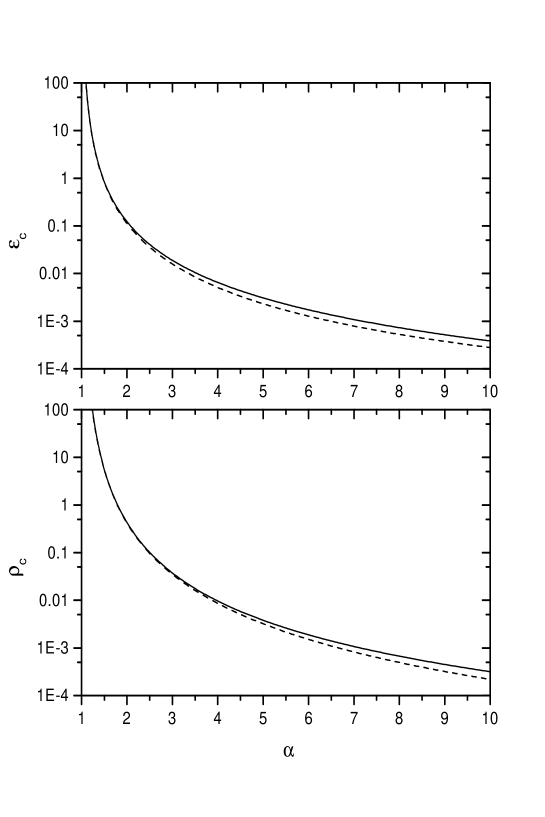
Figure 4: Dimensionless Casimir interaction energy (upper panel) and pressure (lower panel), defined in Eqs.(62) and (65), as a function of $\alpha=b/a$. In both panels the dashed line corresponds to the exact result and the full line to the semiclassical result.

In Fig. 4 we display the exact results (dashed line) together with those corresponding to the semiclassical calculation (full line) as a function of the ratio of the radii of the two cylinders, $\alpha=b/a$. For convenience we have defined the dimensionless energies as

$$\epsilon_{12}=-\frac{a^{2}}{\hbar c}\ \frac{E_{12}}{\ell}\;,\;\;\;\;\;\epsilon^{sem}=-\frac{a^{2}}{\hbar c}\ \frac{E^{sem}}{\ell}\;.$$ (62)

As all energies are defined up to a constant, it is more meaningful to compare the exact and semiclassical pressures on a given cylinder. Specifically, we compare the pressure on the inner cylinder due to the presence of the outer cylinder,

$$p_{12}=-\frac{1}{2\pi a\ell}\frac{\partial E_{12}}{\partial a}\;,$$ (63)

with

$$p^{sem}=-\frac{1}{2\pi a\ell}\frac{\partial E^{sem}}{\partial a}\;.$$ (64)

We also display in Fig. 4 the exact and semiclassical results for the dimensionless pressures

$$\rho_{12}=\frac{2\pi a^{4}}{\hbar c}\ p_{12}\;,\;\;\;\;\;\rho^{sem}=\frac{2\pi a^{4}}{\hbar c}\ p^{sem}\;.$$ (65)

As expected, the discrepancies between the results increases with $\alpha$. One should remark that, as already mentioned, the comparison between the exact and semiclassical energies is subjected to some ambiguities that are not present in the case of the pressures. Therefore, assuming a typical experimental precision of the order of 10 %, such discrepancies would be observable only for values $\alpha>4$ if the pressure would be measured (see Fig.4 lower panel). Thus, it is fair to conclude that, within a typical experimental error, the semiclassical expressions lead to very good results for values of $\alpha$ in the rather wide range $1<\alpha<4$. It should be stressed that, within that range, the Casimir interaction energies and pressures decrease by several orders of magnitude.

The full pressure on the inner cylinder is

$$p_{ex}=-\frac{1}{2\pi a\ell}\frac{\partial E_{ex}}{\partial a}=p_{12}-0.01356{\hbar c\over\pi a^{3}}\;.$$ (66)

For $\alpha\sim 1$ the attraction of the outer cylinder dominates and the full pressure is positive. The inner cylinder tends to expand. However, when $\alpha$ is large, the self-pressure (second term in the above equation) is bigger and the full pressure becomes negative. The crossover takes place at $\alpha\sim 3.15$. It is remarkable that the semiclassical approximation is accurate beyond this critical value.

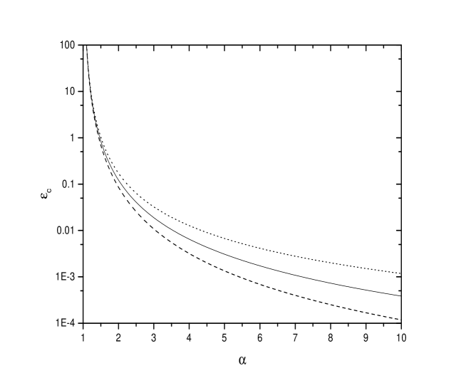
Figure 5: Dimensionless Casimir interaction energy in the semiclassical approximation (full line) as compared to the result obtained using two naive ways of determining the relevant area which enters in the proximity theorem: area of the inner cylinder (dashed line); area of the outer cylinder (dotted line).

Given the good results obtained within the semiclassical approximation it is interesting to consider them in greater detail. We have seen that in the case of the $w=0$ contribution an explicit analytical expression can be obtained for arbitrary values of $\alpha$. One might wonder how well the exact results can be described by this expression. Numerical calculation shows that if one would plot such contribution in Fig. 4 they would be completely indistinguishable from those corresponding to the full semiclassical calculation. In fact, even for $\alpha=10$ the contributions with $w\geq 1$ represents less than 3% of the total value of the energy or pressure. Thus, it is clear that the semiclassical results are completely dominated by the $w=0$ contribution which, in turn, is dominated by the primitive self-retracing orbit $(v=1)$ and its first repetitions $(v=2,3)$. We have also mentioned that the expression corresponding to the $w=0$ contribution, Eq. (29), reduces exactly to that given by the proximity theorem in the limit $\alpha\rightarrow 1$. However, as explained at the end of Sec.III, it is not clear how to extrapolate the use of such theorem away from that limit. The basic problem is that there is an ambiguity on which area should be considered for the differential surfaces. In fact, one might either take the area given by the radius of the inner cylinder, the one given by the radius of the external cylinder or any combination in between (e.g. average radius, geometric mean radius, etc). The situation is illustrated in Fig. 5 where our semiclassical results (full line) are compared with the extrapolation of the proximity theorem using the two extreme alternatives: area given by the inner cylinder (dashed line) and that given by the outer cylinder (dotted line). Obviously, any other sensible choice would lie between these two curves. Although for values of $\alpha$ very close to one this ambiguity is completely harmless, already at such small values $\alpha\approx 1.12$ it implies an uncertainty of the order of 10 %. The present semiclassical calculation removes completely such ambiguity indicating that indeed the geometric mean radius is the right choice.

VI Conclusions

In this article we have computed the Casimir interaction energy for two infinite concentric cylinders exactly and using an approximate semiclassical method. To perform the semiclassical calculation, we have extended the method introduced in Ref.schaden2 , valid for non-symmetric configurations with isolated periodic trajectories, to the case of symmetric configurations in which families of non isolated periodic orbits contribute significantly in the semiclassical limit. Technically, this involves the use of the Balian-Bloch or Berry-Tabor trace formulae instead of the Gutzwiller formula. As for the exact calculation, we have used the mode-by-mode summation method of Ref.piro , but using a cutoff instead of zeta function regularization.

The final result for the semiclassical Casimir energy (Eq.(25)), is dominated by the self-retracing periodic orbit $(w=0)$ and its repetitions. Moreover, it can be interpreted as a proximity approximation with an effective area given by the geometric mean of the areas of both cylinders. While this choice for the area was previously derived for proximity forces in non-symmetric configurations schaden1 ; blocki , the semiclassical calculation provides a justification for the case of an integrable cavity. We have found that, surprisingly, the semiclassical result describes accurately the Casimir pressure beyond the range of validity of the proximity theorem. Indeed, while this theorem is expected to be valid when $b-a\ll a$, the semiclassical result reproduces the exact pressure within a 10 % up to $b=4a$.

As a side point, we remark that the semiclassical approximation fails to reproduce the electromagnetic Casimir energy for an isolated infinite cylinder. Unlike the case of a rectangular parallelepiped schaden2 , the Dirichlet and Neumann contributions have opposite signs. Taking into account that for cavities with axial symmetry, the electromagnetic Casimir energy is the sum of Dirichlet and Neumann scalar contributions, we obtained a vanishing result for the semiclassical energy (other approximations also give a null result for the cylinder bd2 ; maclay ). This shows that the semiclassical method may not work for cavities with one of the dimensions much larger than the others, as was suggested in Ref. schaden2 .

The semiclassical approach described here could be applied to other integrable configurations of conductors, like two concentric spheres. Moreover, it can be extended to incorporate effects that could be relevant experimentally, like small surface deformations or roughness. We are currently investigating these problems.

VII ACKNOWLEDGMENTS

This work was supported by Universidad de Buenos Aires, Conicet, and Agencia Nacional de Promoción Científica y Tecnológica, Argentina.

Appendix A

In this Appendix we describe with some detail the steps followed to obtain the oscillating contributions $\rho^{osc}_{12,I}$ and $\rho^{osc}_{12,II}$, Eqs. (12) and (13).

As we have mentioned in Sec.III the oscillating contribution for non-relativistic particles confined in a bidimensional annular region $\odot$, $\rho^{osc}_{\odot}(E_{m})$, has been previously derived (see e.g. Richter’s book in Ref.brack ). It can been written as a sum of two terms, each one associated respectively to the contributions from type-I and type-II PO’s. In Sec.III we have characterized these PO, whose lengths are $L_{vw}=2\,v\;b\sin(\pi w/v)$ for type-I PO, and $\bar{L}_{vw}=2\,v\;b\;\sqrt{\left(1+\;\left(\frac{a}{b}\right)^{2}\;-2\;\frac{a}{b}\;\cos(\pi w/v)\right)}$ for type-II PO (see the description that precedes Eqs. (10) and (11)). Taking this into account we can write $\rho^{osc}_{\odot}(E_{m})\;=\rho^{osc}_{\odot,I}(E_{m})+\rho^{osc}_{\odot,II}(E_{m})$ with $E_{m}={\hbar\;k}^{2}/2\;m$ brack and

$$\rho^{osc}_{\odot,I}(E_{m}) = \sum_{w\geq 1}\;\sum_{v\geq\hat{v}}\sqrt{\frac{2}{\pi}}\;\frac{m}{{\hbar}^{2}\;k^{1/2}}\;\frac{L_{vw}^{3/2}}{v^{2}}\;\cos\left(k\;L_{vw}\pm\frac{v\;\pi}{2}+\frac{\pi}{4}\right)\;,$$ (67)

$$\rho^{osc}_{\odot,II}(E_{m}) = \sum_{w\geq 0}\;\sum_{v\geq\hat{v}}f_{vw}\;2\sqrt{\frac{2}{\pi}}\frac{b^{2}\;m}{(\hbar)^{2}\;(k\;{\bar{L}_{vw}})^{1/2}}\;A_{vw}\;\sin\left(k\;\bar{L}_{vw}+\;\frac{\pi}{4}\right)\;.$$ (68)

$A_{vw}$ has been defined in Eq.(14). Therefore in order to obtain the oscillating contributions to the density of modes for photons confined in the region $\odot$ we have to replace in Eqs. (67) and (68), ${\hbar\;k}^{2}/2\;m\rightarrow p/c$ and $(\hbar\;k)/m\rightarrow c$. This is trivial and leads to $\rho^{osc}_{\odot,I}(k)$ and $\rho^{osc}_{\odot,II}(k)$ with $k=E/\hbar c$.

To derive the oscillating contribution to the spectral density in the region between the two coaxial cylinders we have to perform the integral Eq.(9), that we write here in a slightly different form,

$$\rho^{osc}_{12,po}(E=\hbar c\;k)=\frac{\ell}{\hbar\;c\pi}\;\int_{0}^{k}\frac{k}{\sqrt{k^{2}-k_{z}^{2}}}\;\rho^{osc}_{\odot,po}(\sqrt{k^{2}-k_{z}^{2}})\;dk_{z}\;,$$ (69)

to emphasize with the subscript $po=I$ or $II$ the contributions from the two types of PO’s. $\rho^{osc}_{\odot,po}(\sqrt{k^{2}-k_{z}^{2}})$ is obtained after replacing $k\rightarrow\sqrt{k^{2}-k_{z}^{2}}$ in $\rho^{osc}_{\odot,I}(k)$ and in $\rho^{osc}_{\odot,II}(k)$. The integrals are straightforward to perform to leading order in $\hbar$, and as a result we obtain Eqs.(12) and (13).

Figure 3: Contour for the integration in the complex plane.

References

- (1) H. B. G. Casimir, Proc. K. Ned. Akad. Wet. 51, 793 (1948); V.M. Mostepanenko and N.N. Trunov, The Casimir effect and its applications, Clarendon, London (1997); M. Bordag, The Casimir effect 50 years later, World Scientific, Singapore (1999); P. Milonni, The quantum vacuum, Academic Press, San Diego (1994); G. Plunien, B. Muller and W. Greiner, Phys. Rep. 134, 87 (1986).
- (2) G. Bressi, G. Carugno, R. Onofrio and G. Ruoso, Phys. Rev. Lett. 88, 041804 (2002).
- (3) S. K. Lamoreaux, Phys. Rev. Lett. 78, 5 (1997).
- (4) U. Mohideen and A. Roy, Phys. Rev. Lett. 81, 4549 (1998); B.W. Harris, F. Chen and U. Mohideen, Phys. Rev. A 62, 052109 (2000).
- (5) H.B. Chan et al., Science 291, 1941 (2001).
- (6) H.B. Chan et al., Phys. Rev. Lett. 87, 1801 (2001).
- (7) M. Bordag, U. Mohideen and V.M. Mostepanenko, Phys. Rep. 353, 1 (2001).
- (8) T.H. Boyer, Phys. Rev. 174, 1764 (1968).
- (9) V.V. Nesterenko and I.G. Pirozhenko, Phys. Rev. D57, 1284 (1997).
- (10) M.E. Bowers and C.R. Hagen, Phys. Rev. D 59, 02007 (1999).
- (11) L.L. DeRaad Jr. and K. Milton, Ann. Phys. (N.Y.)136, 229 (1981).
- (12) K.A. Milton, A.V. Nesterenko and V.V. Nesterenko, Phys. Rev. D 59, 105009 (1999).
- (13) P. Gosdzinsky and A. Romeo, Phys. Lett. B 441, 265 (1998).
- (14) B.V. Derjaguin and I.I. Abriksova, Sov. Phys. JETP 3, 819 (1957); B.V. Derjaguin, Sci. Am. 203, 47 (1960).
- (15) M. Schaden and L. Spruch, Phys. Rev. Lett. 84, 459 (2000).
- (16) A.A. Saharian, Phys. Rev. D63, 125007 (2001)
- (17) A.A. Saharian, ICTP preprint, IC/2000/14.
- (18) See Plunien et al, in Ref[1].
- (19) R. Balian and B. Duplantier, Ann. Phys. 112, 165 (1978)
- (20) M. Schaden and L. Spruch, Phys. Rev. A 58, 935 (1998).
- (21) H. Weyl, Nach. Akad. Wiss. Gõttingen 110, (1911).
- (22) R. Balian and C. Bloch, Ann. Phys. 60, 401 (1970); 63, 592 (1971).
- (23) H. P. Baltes and E. R. Hilf: Spectra of finite systems ( B - I Wissenschaftsverlag, Mannheim, 1976).
- (24) R. Balian and C. Bloch, Ann. Phys. 69, 76 (1972).
- (25) M. V. Berry and M. Tabor, Proc. R. Soc. London, Ser. A. 349, 101 (1976).
- (26) M. C. Gutzwiller in Chaos in Classical and Quantum Mechanics (Springer-Verlag, New York, 1990).
- (27) For a review see for example: M. Brack and R. K. Bhaduri in Semiclassical Physics (Addison-Wesley Publishing Company, Masachussets, 1997); K. Richter in Semiclassical Theory of Mesoscopic Quantum Systems (Springer, Berlin, 2000).
- (28) R. Balian and B. Duplantier, Ann. Phys. 104, 300 (1977).
- (29) M. J. Sánchez, unpublished.
- (30) J. Blocki, J. Randrup, W.J. Swiatecki and F. Tsang, Ann. Phys.105, 427 (1977).
- (31) For simplicity, to compute the limit we assumed . The final result for the Casimir energy does not depend on this particular choice.
- (32) G.J. Maclay, H. Fearn, P. W. Milonni quant-ph/0105002