Diffusive-ballistic Crossover in 1D Quantum Walks

Abstract

We show that particle transport, as characterized by the equilibrium mean square displacement, in a uniform, quantum multi-baker map, is generically ballistic in the long time limit, for any fixed value of Planck’s constant. However, for fixed times, the semi-classical limit leads to diffusion. Random matrix theory provides explicit analytical predictions for the mean square displacement of a particle in the system. These results exhibit a crossover from diffusive to ballistic motion, with crossover time on the order of the inverse of Planck’s constant. This diffusive behavior is a property of the equilibrium average and does not require further interactions of the system with the environment. We expect that, for a large class of 1D quantum random walks similar to the quantum multi-baker, a sufficient condition for diffusion in the semi-classical limit is classically chaotic dynamics in each cell. These results describe an interesting generalization of known quantum random walks and may have applications for quantum computation.

Recent results for non-equilibrium and transport properties of extended classical systems with microscopic chaos Dorfman (1999); Gaspard (1998) have suggested that one might explore the transport behavior of quantum versions of simple, extended classical systems. One such system, studied here, is the multi-baker model for deterministic diffusion in one-dimension. In paper Wójcik and Dorfman (2002a) we introduced a quantum version of the classical multi-baker model as a combination of local quantum baker dynamics with a transport of wave functions to neighboring cells. Its simplest case is an example of the quantum random walks that have been considered previously (the Hadamard walk) Godoy and Garcia-Colin (1996); Travaglione and Milburn (2002), but other cases form a much wider class of 1D quantum random walks. Quantum random walks have become of considerable interest over the past few years since they might be useful for implementing quantum random search algorithms if quantum computation becomes possible. Quantum multi-baker models might be excellent candidates for implementation as part of current efforts to provide techniques and algorithms designed to take advantage of the possibilities inherent in quantum computation. Its experimental realization eventually may be feasible since both quantum baker maps Brun and Schack (1999); Weinstein et al. (2002), and the Hadamard walks Travaglione and Milburn (2002), are now within experimental reach. The general case we consider allows a larger number of quantum states participating in the random walk, and widens the range of possible physical applications.

In this Letter we report on the behavior of the equilibrium mean square displacement (m.s.d.) for a quantum particle whose classical dynamics is governed by the deterministic, diffusive multi-baker process. Since one-dimensional processes in extended quantum systems show ballistic motion, for translationally invariant systems, or localization, for disordered ones, it is interesting to study how each system makes the transition to diffusive behavior in the classical limit. Here we concentrate on the translationally invariant case. A natural question is whether or not an interaction with the external world, or decoherence, is necessary to eventually restore diffusive motion in the classical limit. Our work here shows that this is not the case for the m.s.d.: for systems that we study there is a crossover from short-time diffusive behavior to ballistic motion in the long time limit. The crossover time is on the order of the inverse Planck constant, i.e. the Heisenberg time, rather than the Ehrenfest time, on the order of the log of Planck’s constant. The chaotic classical motion of our system allows the use of random matrix theory (RMT), which leads to explicit expressions for the mean square displacement of a quantum particle. The comparison of the RMT analytic results with results of numerical evaluation of the exact formula for particular systems is very good with some interesting exceptions. Our calculation has a classical counterpart Gaspard (1998) which has the same result for the m.s.d. as obtained here in the semi-classical limit.

We begin with the classical multi-baker map Gaspard (1992); Tasaki and Gaspard (1995). It is a deterministic model of the random walk on a one-dimensional lattice, where the direction of the jump is determined by the internal state of the particle. We use the baker map as a model of internal dynamics. That is, the multi-baker map, $M$, is a composition of two maps $M=B\circ T$. First, the phase points are transported to neighboring cells according to $T(n,x,y)=(n+1,x,y)$, for $0\leq x<1/2$, and $(n-1,x,y)$ for $1/2\leq x<1$. Then a baker map $B$ acts on the $x,y$ coordinates of each cell, $n$, separately, according to $B(n,x,y)=(n,2x,y/2)$, for $0\leq x<1/2$, and $(n,2x-1,(1+y)/2)$, for $1/2\leq x<1$. The combination of these two maps is the multi-baker map which is a time-reversible, measure preserving, chaotic transformation, with evolution law

$$M(n,x,y)=\left\{\begin{array}[c]{ll}(n+1,2x,\frac{y}{2}),&\,{\rm for}\;0\leq x<1/2,\\ (n-1,2x-1,\frac{1+y}{2}),&\,{\rm for}\;1/2\leq x<1.\end{array}\right.$$

It is the simplest area-preserving model of a random walk.

To quantize the dynamics we first quantize $B$ in a single cell. The horizontal direction of the torus $[0,1)^{2}$ is taken to be the coordinate axis, while vertical axis corresponds to the momentum direction. To obtain the Hilbert space Hannay and Berry (1980); Saraceno (1990); DeBievre et al. (1996) we take the subspace of the wave functions on a line whose probability densities, $|\Psi(x)|^{2},|\tilde{\Psi}(p)|^{2}$ are periodic in both position and momentum representations, respectively: $\Psi(x+1)=\exp(i2\pi\varphi_{q})\Psi(x)$, $\tilde{\Psi}(p+1)=\exp(i2\pi\varphi_{p})\tilde{\Psi}(p)$, where $\varphi_{q},\varphi_{p}\in[0,1)$ are phases parameterizing quantization. The quantization of the baker map requires the phase space volume to be an integer multiple of the quantum of action Hannay and Berry (1980); Saraceno (1990); DeBievre et al. (1996), so the effective Planck constant must be $h=1/N$, where $N$ is the dimension of the Hilbert space. The space and momentum representations are connected by a discrete Fourier transform $G_{N}(\varphi_{q},\varphi_{p}):=\langle p_{k}|q_{l}\rangle={N}^{-1/2}\exp(-i2\pi Np_{k}q_{l})$. The discrete positions and momenta are $q_{l}=(l+\varphi_{q})/N$, $p_{k}=(k+\varphi_{p})/N$. The Hilbert space $H$ can be decomposed into “left” and “right” subspace $H=H_{L}\oplus H_{R}$, and “bottom”/“top” spaces $H=H_{B}\oplus H_{T}$, which are $N/2$ dimensional, $\Psi\in H_{L}$ when $\langle q_{l}|\Psi\rangle=0$ for $l=N/2,\dots,N-1$, $\Psi\in H_{B}$ when $\langle p_{k}|\Psi\rangle=0$ for $k=N/2,\dots,N-1$.

Having constructed the Hilbert space one looks for a family of unitary propagators parameterized by $N=1/h$ which go over into the classical map in semi-classical limit. Technically, one requires the Egorov condition to be satisfied, which means semi-classical commutation of the quantum and classical evolution DeBievre et al. (1996). The unitary operator for the quantum baker map Balazs and Voros (1989); Saraceno (1990); DeBievre et al. (1996) is given by $U_{N}:=G_{N}^{-1}\left[\begin{array}[c]{cc}G_{N/2}&0\\ 0&G_{N/2}\end{array}\right]$ for even $N$. Other examples and discussions of issues concerning the quantization of area-preserving maps can be found e.g. in Bäcker (2002).

Since the quantum multi-baker is a model of particle with $N$ internal states jumping over lattice of length $L$, we use product Hilbert space $H={\mathbb{C}}^{L}\otimes{\mathbb{C}}^{N}$ to describe it. The dynamics is implemented in two steps. First one shifts states from right subspace at cell $n$ ($H_{R}(n)$)to right states at cell $n-1$, and states $H_{L}(n)$ into left states at cell $n+1$, which gives the quantum transport operator $T$. Then on each of the cells one acts independently with a quantum baker operator $U_{N}$, which corresponds to the classical map $B$. Let us write the states $|\Psi\rangle\in H$ in the position basis $\sum_{n=0}^{L-1}\sum_{j=0}^{N-1}\Psi_{j}(n)|n,j\rangle$. Then the only non-zero matrix elements of the quantum multi-baker operator $M$ are of the form $\langle n+1,j|M|n,k\rangle=\langle j|U_{N}|k\rangle$, for $k\in H_{L}(n)$, or $\langle n-1,j|M|n,k\rangle=\langle j|U_{N}|k\rangle$, for $k\in H_{R}(n)$. For the translationally invariant case studied here, the m.s.d. can be expressed entirely in terms of the properties of the baker operator, $B$, cf. Eq. (2), and we do not need to make explicit use of the structure of $M$.

The central quantity of interest, is the expression for the mean square displacement (m.s.d.) of a quantum particle in the chain, defined as the average value of the mean square displacement taken with an equilibrium density matrix for the system. This is a uniform distribution of probabilities along the chain, $\varrho_{eq}={\mathbb{I}}_{NL}/NL$; $\langle A\rangle:=\mbox{\rm Tr}\ (\varrho_{eq}A)=\mbox{\rm Tr}\ (A)/NL$, $L$ is the length of the chain (we assume periodic boundary conditions and where $N$ is the dimension of the Hilbert space. Then the m.s.d. is simply $\langle(\Delta r)^{2}(t)\rangle=\langle(M^{\dagger t}rM^{t}-r)^{2}\rangle$. If we define the velocity operator $v:=M^{\dagger}rM-r$ then the m.s.d. can be written as $\langle(\Delta r)^{2}(t)\rangle=\sum_{m,n=0}^{t-1}\langle v_{m}v_{n}\rangle$, where $v_{n}:=M^{\dagger n}vM^{n}$. Time invariance of $\varrho_{\rm eq}$ implies $\langle v_{m}v_{n}\rangle=\langle v_{m-n}v_{0}\rangle$. Thus we can express the m.s.d. in terms of the velocity autocorrelation function $C_{n}=\langle v_{n}v_{0}\rangle$:

$$\langle(\Delta r)^{2}(t)\rangle=t\langle v^{2}\rangle+2\sum_{n=1}^{t-1}(t-n)C_{n}$$ (1)

We use a “coarse” position operator $r$ defined by $r|n,k\rangle:=n|n,k\rangle$. We calculate the coarse velocity operator on the line using the definition given above, obtaining Wójcik and Dorfman (2002b), $v(n,k;m,l)=\pm\delta_{k,l}\delta_{n,m}$, with $+$ for $l<N/2$, $-$ for other $l$, and then put it on the circle to enforce translational invariance. This form can be understood by observing that for the translationally invariant case, the coarse velocity $\pm 1$ denotes a translation of the quantum state one cell to the right or left. An identical form for the coarse velocity occurs in the classical multi-baker as well Dorfman (1999). Then the velocity autocorrelation function can be reduced to the trace over states in a single cell Wójcik and Dorfman (2002b)

$$C_{n}=\frac{1}{LN}\mbox{\rm Tr}\ [M^{\dagger n}vM^{n}v]=\frac{1}{N}\mbox{\rm Tr}\ [B^{\dagger n}JB^{n}J],$$ (2)

where we note that $J$ is the velocity operator $v$ reduced to a single cell. In the position representation $J$ is given by $J=\left(\begin{array}[]{cc}\mathbb{I}_{N/2}&0\\ 0&-\mathbb{I}_{N/2}\end{array}\right).$ Assuming the properties of the local propagator, $B$, are known, one can express the velocity autocorrelation function in terms of its spectrum and eigenvectors, where $B|k\rangle=\exp(i\varphi_{k})|k\rangle$. It immediately follows that

$$C_{n}=\frac{1}{N}\sum_{j,k}|J_{jk}|^{2}e^{i(\varphi_{j}-\varphi_{k})n},$$ (3)

where $J_{jk}:=\langle j|J|k\rangle$. Since $J$ has a very simple form, one sees that

$$\sum_{j,k}|J_{jk}|^{2}=\mbox{\rm Tr}\ J^{2}=N.$$ (4)

Substituting these results in formula (1) we obtain

$$\langle(\Delta r)^{2}(t)\rangle = \frac{1}{N}t\sum_{j\neq k}|J_{jk}|^{2}+\frac{1}{N}t^{2}\sum_{j}|J_{jj}|^{2}$$ (5)

$$+\frac{2}{N}\sum_{j\neq k}|J_{jk}|^{2}\sum_{n=1}^{t-1}(t-n)\,e^{i\alpha_{jk}n}$$

$$= \frac{t^{2}}{N}\sum_{j}|J_{jj}|^{2}+\sum_{j\neq k}\frac{|J_{jk}|^{2}}{N}\frac{\sin^{2}\frac{(\alpha_{jk}t)}{2}}{\sin^{2}\frac{\alpha_{jk}}{2}}$$ (6)

where $\alpha_{jk}:=\varphi_{j}-\varphi_{k}$. Whenever there is a degeneracy, $\alpha_{jk}=0$, we replace the ratio of sines by $t^{2}$. In certain cases it is possible that the coefficient of the ballistic, $t^{2}$, term may be zero; see Figure 2.b and the following discussion.

We now evaluate the m.s.d., Eq. (5) using random matrix theory and compare the results with numerical evaluations. To apply RMT we consider the velocity autocorrelation function $C_{n}$ given by Eq. (3), and separate the terms on the right hand side into diagonal, $j=k$, and non-diagonal, $j\neq k$, terms. We suppose that $B$ is drawn randomly from either the COE or CUE ensembles, although the numerical results present a more general behavior. We assume the distribution of matrix elements is independent of the distribution of elements of eigenvectors (see section 8.2 of Haake (2001), and Kuś et al. (1988)). Using $\mbox{\rm Tr}J^{2}=N$, one sees that the ensemble average of the mean square displacement takes the form

$$\langle\langle(\Delta r)^{2}\rangle\rangle = t+t(t-1)\langle|J_{jj}|^{2}\rangle$$ (7)

$$+2(N-1)\langle|J_{j\neq k}|^{2}\rangle\sum_{n=1}^{t-1}(t-n)\,\langle e^{i\alpha n}\rangle.\qquad\$$

We replace the matrix elements $|J_{jj}|^{2}$ and $|J_{jk}|^{2}$ by their average values $\langle|J_{jj}|^{2}\rangle$ and $\langle|J_{jk}|^{2}\rangle$, respectively. Straightforward calculation Wójcik and Dorfman (2002b) gives $\langle|J_{jj}|^{2}\rangle=k/(N+k)$, where $k=1$ for CUE, and 2 for COE. Averaging Eq. (4), we obtain $\langle|J_{jj}|^{2}\rangle+(N-1)\langle|J_{j\neq k}|^{2}\rangle=1$ and thus $\langle|J_{j\neq k}|^{2}\rangle=N/[(N+k)(N-1)]$. Then we need to calculate the average value of the exponential factor $\exp[i(\varphi_{j}-\varphi_{k})n]$. For this calculation we need the expression for the pair correlation function $R(\varphi_{j},\varphi_{k})$ in the two ensembles, so that we can express the average value as

$$\langle e^{[i(\varphi_{i}-\varphi_{k})n]}\rangle=\int_{0}^{2\pi}\!\!\int_{0}^{2\pi}\!\!d\varphi_{j}\,d\varphi_{k}\,e^{[i(\varphi_{i}-\varphi_{k})n]}\,\frac{R(\varphi_{j},\varphi_{k})}{N(N-1)}.$$

These correlation functions are given in the literature Mehta (1991). For the CUE, one finds that

$$R(\varphi_{j},\varphi_{k})=\frac{N^{2}}{4\pi^{2}}\left[1-\frac{\sin^{2}\frac{N(\varphi_{j}-\varphi_{k})}{2}}{N^{2}\sin^{2}\frac{(\varphi_{j}-\varphi_{k})}{2}}\right].$$

A straightforward calculation Wójcik and Dorfman (2002b), leads to

$$\langle e^{[i(\varphi_{j}-\varphi_{k})n]}\rangle=\left\{\begin{array}[c]{ll}1&\,{\rm for}\;n=0\\ \frac{n-N}{N(N-1)}&\,{\rm for}\;n<N,\\ 0&\,{\rm for}\;n\geq N.\end{array}\right.$$ (8)

Using this estimate for the average the result, we find that the m.s.d. is given by

$$\langle(\Delta r)^{2}(t)\rangle=\left\{\begin{array}[c]{ll}t+\frac{t(t-1)}{N+k}\left[k-1+\frac{t-2}{3(N-1)}\right]&\,{\rm for}\;t\leq N,\\ \frac{k}{N+k}t^{2}+\frac{N}{3}-\frac{N(k-1)}{3(N+k)}&\,{\rm for}\;t>N.\end{array}\right.$$

Note that the “super-ballistic” $t^{3}$ term only occurs for $t\leq N$, where it is typically less than or on the order of the linear term, $t$. The exact result for the COE ensemble has a correction arising from an additional term in the pair correlation function. This correction is rather lengthy to write and is negligible for both short and very long times, with the maximum deviation of at most five percent occurring at $t=N$. The details will be given elsewhere Wójcik and Dorfman (2002b). Figure 1 shows the estimates for the two ensembles for $N=200$.

Figure 1: Log-log plot of the ensemble averages of the mean square displacement using RMT. The COE results are the two close curves, where the lower is the result given in Eq. (8) for $k=2$, while the higher curve was obtained using the full pair correlation function for COE. Three asymptotic estimates $t,t^{2}/N,2t^{2}/N$ are also plotted. The inset shows the region $t=100$ to $t=300$ where the differences between the two COE results are most pronounced.

We compare these predictions with numerical results. For almost every choice of phases $\varphi_{q},\varphi_{p}$ defining the quantization, the evaluated formula (6) gives results between the COE and CUE average predictions for $N$ greater than 100. The Balazs-Voros phases ($\varphi_{q}=\varphi_{p}=0$) Balazs and Voros (1989) yield exceptionally good agreement with CUE average for all values of $N$.

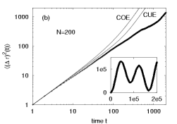
Figure 2: Comparison of RMT estimates with the numerical evaluation of the formula (6) for the m.s.d. in case of quantum multi-bakers with a) Balazs-Voros phases (generic case), b) Saraceno phases (exceptional, localized case). Plots are in double logarithmic scale, the inset in figure (b) shows the results for much longer time in normal scale.

Figure (2.a) compares the exact result with the RMT averages in this case.

An interesting exception to these results occurs when $\varphi_{q}+\varphi_{p}=1$, e.g. for the Saraceno case ($\varphi_{q}=\varphi_{p}=1/2$) Saraceno (1990). For these special values of the phases, the probability of finding the system on each half is 0.5 for every eigenstate, so that $J_{jj}=0$, and there are no degeneracies. Thus for long times the m.s.d. oscillates around the time average value, $\sum_{j\neq k}|J_{jk}|^{2}/(2N\sin^{2}\frac{\alpha_{jk}}{2})$, after an initial diffusive growth. To see how such oscillations are possible, consider a more general class of systems where the local quantum baker map is replaced by an arbitrary unitary operator $B$ Wójcik and Dorfman (2002b). For this larger class of systems one easily proves that $0\leq\langle(\Delta r)^{2}\rangle\leq t^{2}$, both classically and quantum-mechanically, and it is easy to construct examples realizing both extrema. Moreover, if $B$ is a right-left exchange operator, which merely replaces left and right states, the m.s.d. oscillates between 0 and 1. Similar phenomena over much longer time-scales may take place in the case discussed above. Figure (2.b) shows reasonable agreement with the short-time classical diffusive behavior also in the case of Saraceno quantization. We expect that for large $N$ the phases should not matter for times up to the Heisenberg time.

Summary: We have considered the mean square displacement of a particle whose dynamics is governed by the propagator for a quantum multi-baker map. After deriving a general formula for the m.s.d., we evaluated it by means of RMT and also by numerical methods. Random matrix theory provides explicit, analytic expressions for the m.s.d., as well as for the velocity autocorrelation functions that determine it. Our study shows that these analytic expressions depend somewhat on the nature of the circular ensembles used, either unitary or orthogonal. Comparison with numerical results shows that neither of the ensembles is superior: depending on quantization phases one or the other gives a better representation of the data, but usually the experimental curve lies between the two predictions with numerical ballistic coefficient having values between $1/N$ and $2/N$ for generic (ballistic) systems. The analytic expressions for the m.s.d. allow us to study the transition to classical behavior in detail. We find that, on the average, there is a smooth transition from quantum to classical behavior as Planck’s constant approaches zero, and that for non-zero values of $h$ the classical behavior persists up to times on the order of $h^{-1}$, and we see no need for further interactions with the environment, for a well behaved classical limit for the models we study. Thus the analytic expressions for the velocity autocorrelation functions and m.s.d. provide a powerful tool for studying the quantum-classical transition for simple extended systems. Given that it is possible to realize a quantum baker map experimentally, the quantum multi-baker map eventually may have applications for quantum computations.

We show elsewhere that most of the results presented here are valid for a much wider class of quantum systems Wójcik and Dorfman (2002b).

The authors would like to thank S. Fishman, P. Gaspard, M. Kuś, J. P. Paz, S. Tasaki, J. Vollmer, and K. Życzkowski for helpful comments, and the National Science Foundation for support under grant PHY-98-20824.

References

- Dorfman (1999) J. R. Dorfman, An introduction to chaos in nonequilibrium statistical mechanics (Cambridge University Press, Cambridge, 1999).
- Gaspard (1998) P. Gaspard, Chaos, scattering and statistical mechanics (Cambridge University Press, Cambridge, 1998).
- Wójcik and Dorfman (2002a) D. K. Wójcik and J. R. Dorfman, Phys. Rev. E 66, 036110 (2002a).
- Godoy and Garcia-Colin (1996) S. Godoy and L. S. Garcia-Colin, Phys. Rev. E 53, 5779 (1996); A. Ambainis, et al., in Proceedings of the 30th STOC (ACM, 2001), pp. 37–49.
- Travaglione and Milburn (2002) B. C. Travaglione and G. J. Milburn, Phys. Rev. A 65, 032310 (2002); W. Dür, R. Raussendorfer, V. M. Kendon, and H.-J. Briegel (2002), quant-ph/0207137.
- Brun and Schack (1999) T. A. Brun and R. Schack, Phys. Rev. A 59, 2649 (1999).
- Weinstein et al. (2002) Y. S. Weinstein, S. Lloyd, J. Emerson, and D. G. Cory, Phys. Rev. Lett. 89, 157902 (2002).
- Gaspard (1992) P. Gaspard, J. Stat. Phys. 68, 673 (1992).
- Tasaki and Gaspard (1995) S. Tasaki and P. Gaspard, J. Stat. Phys. 81, 935 (1995).
- Hannay and Berry (1980) J. H. Hannay and M. V. Berry, Physica D 1, 267 (1980).
- Saraceno (1990) M. Saraceno, Ann. Phys. 199, 37 (1990).
- DeBievre et al. (1996) S. DeBievre, M. D. Esposti, and R. Giachetti, Commun. Math. Phys. 176, 73 (1996).
- Balazs and Voros (1989) N. L. Balazs and A. Voros, Ann. Phys. 190, 1 (1989).
- Bäcker (2002) A. Bäcker (2002), nlin.CD/0204061.
- Wójcik and Dorfman (2002b) D. K. Wójcik and J. R. Dorfman (2002b), in preparation, and nlin.CD/0212036.
- Haake (2001) F. Haake, Quantum Signatures of Chaos (Springer Verlag, Berlin, New York, 2001), 2nd ed.
- Kuś et al. (1988) M. Kuś et al., J. Phys. A 21, L1073 (1988).
- Mehta (1991) M. L. Mehta, Random matrices (Academic Press, New York, 1991).