Trapped-Ion Quantum Simulator: Experimental Application to Nonlinear Interferometers

Abstract

We show how an experimentally realized set of operations on a single trapped ion is sufficient to simulate a wide class of Hamiltonians of a spin-1/2 particle in an external potential. This system is also able to simulate other physical dynamics. As a demonstration, we simulate the action of an $n$-th order nonlinear optical beamsplitter. Two of these beamsplitters can be used to construct an interferometer sensitive to phase shifts in one of the interferometer beam paths. The sensitivity in determining these phase shifts increases linearly with $n$, and the simulation demonstrates that the use of nonlinear beamsplitters ($n$=2,3) enhances this sensitivity compared to the standard quantum limit imposed by a linear beamsplitter ($n$=1).

One of the motivations behind Feynman’s proposal for a quantum computer [1] was the possibility that one quantum system could efficiently simulate the behavior of other quantum systems. This idea was verified by Lloyd [2] and further explored by Lloyd and Braunstein [3] for a conjugate pair of variables such as position and momentum of a quantum particle. Following this suggestion we show below that coherent manipulation of the quantized motional and internal states of a single trapped ion using laser pulses can simulate the more general quantum dynamics of a single spin-1/2 particle in an arbitrary external potential. Previously, harmonic and anharmonic oscillators have been simulated in NMR [4].

In addition to demonstrating the basic building blocks for simulating such arbitrary dynamics, we experimentally simulated the action of optical Mach-Zehnder interferometers with linear and nonlinear second- and third-order beam-splitters on number-states. Interferometers with linear beamsplitters and nonclassical input states have engendered considerable interest, since their noise limits for phase estimation can lie below the standard quantum limit for linear interferometers with coherent input modes [5, 6, 7, 8] as has been demonstrated in experiments [9]. A number of optics experiments have exploited the second-order process of spontaneous parametric down-conversion [10], which can be regarded as a nonlinear beamsplitter. By cascading this process, a fourth-order interaction has also recently been realized [11]. One difficulty in these experiments is the exponential decrease in efficiency as the order increases, necessitating data post-selection and long integration times. In the simulations reported here, nonlinear interactions were implemented with high efficiency, eliminating the need for data post-selection and thereby requiring relatively short integration times.

To realize a quantum computer for simulating a spin $s=1/2$ particle of mass $\mu$ in an arbitrary potential, one must be able to prepare an arbitrary input state

$$|\Psi(m_{s},z)\rangle=\sum_{n}(c_{\downarrow n}|\downarrow\rangle|n\rangle+c_{\uparrow n}|\uparrow\rangle|n\rangle),$$ (1)

where the particle’s position wavefunction is expanded in energy eigenstates $|n\rangle$ of a suitable harmonic oscillator and $|m_{s}\rangle$ ($m_{s}\in\{\downarrow,\uparrow\}$) represent the spin eigenstates in a suitable basis. We have recently demonstrated a method to generate arbitrary states of the type in Eq.(1) in an ion trap [12, 13]. The computer should then evolve the state according to an arbitrary Hamiltonian

$$H = \left[\frac{p^{2}}{2\mu}+V(z,m_{s})\right]$$ (2)

$$\simeq \sum_{n,m\leq n}^{N}(\alpha_{nm}I+\beta_{nm}\sigma_{+}+\beta^{*}_{nm}\sigma_{-}+\gamma_{nm}\sigma_{z})$$ (3)

$$\times (\chi_{nm}(a^{\dagger})^{n}a^{m}+\chi^{*}_{nm}(a^{\dagger})^{m}a^{n}),$$ (4)

where we require only that the potential $V(z,m_{s})$ can be expanded as a power series in the harmonic oscillator ladder operators $a$ and $a^{\dagger}$ and be approximated to arbitrary precision by a finite number of terms with maximum order $N$. The $m_{s}$ are a set of observables in a general two-level Hilbert space that can all be mapped to a linear combination of the indentity $I$ and the Pauli matrices $\sigma_{j}$. The operators $\sigma_{\pm}$ are defined as $\sigma_{\pm}=\sigma_{x}\pm i\sigma_{y}$, all $\beta_{nm},\chi_{nm}$ are complex numbers, and all $\alpha_{nm},\gamma_{nm}$ are real numbers.

In our realization of an analog quantum computer we consider the Hamiltonian of a trapped atom of mass $\mu$, harmonically bound with a trap frequency $\omega_{z}$ and interacting with two running-wave light fields having a frequency difference $\Delta\omega$ and a phase difference $\varphi$ at the position of the ion. Both light fields are assumed to be detuned from an excited electronic level so they can induce stimulated-Raman transitions between combinations of two long-lived internal electronic ground-state levels with energy difference $\hbar\omega_{0}$ and the external motional levels of the ion[14]. For our purpose it is sufficient to consider the motion along one axis in the trap. After applying a rotating wave approximation and adiabatic elimination of the near resonant excited state [14], and switching to an interaction picture of the ion’s motion, the resonant interaction for Raman beam detuning $\Delta\omega=\epsilon\hskip 1.0pt\omega_{0}+l\omega_{z}$ ($\epsilon=\{0,1\}$, $l$ integer) can be written in the Lamb-Dicke limit ($\eta^{2}\langle(a+a^{\dagger})^{2}\rangle\ll 1$) as [15, 16]

$$H_{\epsilon l}=\hbar\Omega e^{i\phi}(\sigma_{+})^{\epsilon}\left[\delta_{l,|l|}\frac{(i\eta a)^{|l|}}{|l|!}+(1-\delta_{l,|l|})\frac{(i\eta a^{\dagger})^{|l|}}{|l|!}\right]+h.c.$$ (5)

The coupling strength $\Omega$ is assumed to be small enough to resonantly excite only the $l$-th spectral component. The Lamb-Dicke parameter $\eta=\Delta k~{}z_{0}$ is the product of the $z$-projection of the wavevector-difference $\Delta k$ of the two light fields and the spatial extent of the ground state wave function $z_{0}=\sqrt{\hbar/(2m\omega_{z})}$. For $\epsilon=1$ the internal state changes during the stimulated Raman transition and the interaction couples $|\downarrow\rangle|n\rangle\leftrightarrow|\uparrow\rangle|n+l\rangle$, while for $\epsilon=0$ only motional states $|n\rangle\leftrightarrow|n+l\rangle$ are coupled with a strength independent of the internal state [17].

Following Lloyd and Braunstein [3, 18], by nesting and concatenating sequences of $H_{\epsilon l}$ operations according to the relation

$$e^{-\frac{i}{\hbar}H\delta t}e^{-\frac{i}{\hbar}H^{\prime}\delta t}e^{\frac{i}{\hbar}H\delta t}e^{\frac{i}{\hbar}H^{\prime}\delta t}=e^{\frac{1}{\hbar^{2}}[H,H^{\prime}]\delta t^{2}}+O(\delta t^{3}),$$ (6)

the set of operators $\{H_{01},H_{02},H_{03},H_{10},H_{11},H_{12},H_{13}\}$ is sufficient to efficiently generate arbitrary Hamiltonians. This conclusion is straightforward for the spin, since $\{\sigma_{+},\sigma_{-},\sigma_{z}\}$ are a complete basis of that algebra. For interactions that only involve the motion ($\epsilon=0$) it follows from the fact that

$$\left[H_{02},H_{03}\right]\propto i\left\{\alpha a^{\dagger}a^{2}+\alpha^{*}(a^{\dagger})^{2}a\right\}+{\rm lower~{}orders}$$ (7)

and

$$\left[\alpha a^{\dagger}a^{2}+\alpha^{*}(a^{\dagger})^{2}a,\beta(a^{\dagger})^{n}a^{m}+\beta^{*}(a^{\dagger})^{m}a^{n}\right]=$$ (8)

$$(2m-n)\left[\alpha\beta(a^{\dagger})^{m}a^{n+1}+\alpha\beta^{*}(a^{\dagger})^{n}a^{m+1}-h.c.\right]$$ (9)

$$+{\rm~{}lower~{}orders},$$ (10)

so one can build up arbitrary orders in the effective Hamiltonian by recursive use of Eq.(6). Similar arguments hold for the set of $\{H_{1l}\}$ interactions, and by combining both types of interactions, the series expansion of the Hamiltonian in Eq.(2) can eventually be constructed.

Most of these interactions have been demonstrated in previous ion-trap experiments. $H_{10}$ is usually called the carrier interaction, $H_{01}$ and $H_{02}$ are coherent and squeeze drives respectively and $H_{11},H_{12}$ are first and second blue sideband [19, 20]. The third-order interactions $H_{03},H_{13}$ have not been previously demonstrated. One of the experiments discussed below uses two $H_{13}$ pulses, therefore demonstrating the feasibility of generating $H_{03}$ as well [21].

As a demonstration of quantum simulation using a single trapped atom, we employ the interactions $H_{11},H_{12}$, and $H_{13}$ to efficiently simulate a certain class of $n$-th order optical beamsplitters described by Hamiltonians

$$B_{n}=\hbar\Omega_{n}[a(b^{\dagger})^{n}+a^{\dagger}(b)^{n}].$$ (11)

Here $a$ and $b$ are the usual harmonic oscillator lowering operators for the two quantized light modes, $\Omega_{n}$ is the coupling strength, and we simulate the special case where the number of photons in mode $a$ is 0 or 1 and $n=1,2$ or 3. Two such beamsplitters can be used to construct a Mach-Zehnder interferometer as sketched in Fig. 1. The order $n=1$ corresponds to the commonly used linear beamsplitter that is typically realized by a partially transparent mirror in experiments. Such interferometers can measure the relative phase of the two paths of the light fields that are split on the first beamsplitter and recombined on the second. The phase can be varied by changing a phase shifting element (the box labeled $\phi$ in Fig. 1) and detected (modulo $2\pi$) by observing the interference fringes of the recombined fields. We restrict our attention to a pure number-state $|n=1\rangle_{a}$ impinging on the first beamsplitter from mode $a$ and a vacuum state $|n=0\rangle_{b}$ from mode $b$. After propagating the input state through the first beamsplitter with $\Omega_{n}$ adjusted to give equal amplitude along the two paths in the output superposition, the state becomes

$$|1\rangle_{a}|0\rangle_{b}\rightarrow\frac{1}{\sqrt{2}}(|1\rangle_{a^{\prime}}|0\rangle_{b^{\prime}}+|0\rangle_{a^{\prime}}|n\rangle_{b^{\prime}}).$$ (12)

Phase shifters in optical interferometers alter a classical-like coherent state $|\alpha\rangle$ to one that is shifted to $|\alpha e^{i\phi}\rangle$. In the context of Fig.1 this phase shift corresponds to $|n\rangle\rightarrow e^{in\phi}|n\rangle$ for a number state, leading to

$$\frac{1}{\sqrt{2}}(|1\rangle_{a^{\prime}}|0\rangle_{b^{\prime}}+|0\rangle_{a^{\prime}}|n\rangle_{b^{\prime}})\rightarrow$$ (13)

$$\frac{1}{\sqrt{2}}(|1\rangle_{a^{\prime}}|0\rangle_{b^{\prime}}+e^{in\phi}|0\rangle_{a^{\prime}}|n\rangle_{b^{\prime}}).$$ (14)

The second beamsplitter recombines the two field modes leading to an average probability of

$$\langle\hat{n}_{a^{\prime\prime}}\rangle=\frac{1}{2}[1-\cos(n\phi)]$$ (15)

for detecting one photon in the output arm with the detector in Fig.1.

We have experimentally simulated the nonlinear beam-splitter of Eq.(11) using a single trapped ⁹Be⁺ ion. The operator $a$ is replaced by $\sigma^{+}$, the raising operator between two hyperfine states $|F=2,m_{F}=-2\rangle\equiv|1\rangle_{a}$ and $|F=1,m_{F}=-1\rangle\equiv|0\rangle_{a}$ in the ²S_1/2 ground state manifold. These operators (and also their respective Hermitian conjugates) are not strictly equivalent, but their action is the same as long as we restrict our attention to situations that never leave the $\{|0\rangle_{a},|1\rangle_{a}\}$ subspace. The simulated linear and nonlinear interferometers fulfill this restriction, as long as the input state is $|1\rangle_{a}|0\rangle_{b}$. The optical mode with lowering operator $b$ is replaced by the equivalent harmonic oscillator mode of motion along one axis in the trap, with number states $|n\rangle$.

Our experimental system has been described in detail elsewhere [19, 20, 22]. We trapped a single ⁹Be⁺ ion in a linear trap [23] with motional frequency $\omega_{z}=2\pi$ 3.63 MHz (Lamb-Dicke parameter $\eta=$0.35) and cooled it to the ground state of motion. The trap had a heating rate of 1 quantum per 6 ms [23] that was a small perturbation for the duration of our experiments ($\leq$ 260 $\mu$s). After cooling, the ion was prepared in the $|1\rangle_{a}|0\rangle_{b}$ state by optical pumping. Starting from this state we used Raman-transitions to drive a $\pi/2$-pulse on the ion’s $n$-th blue sideband ($H_{I}\propto\sigma^{+}(b^{\dagger})^{n}+h.c.$), creating the state $(|1\rangle_{a^{\prime}}|0\rangle_{b^{\prime}}+|0\rangle_{a^{\prime}}|n\rangle_{b^{\prime}})/\sqrt{2}$. For different orders $n$ the $\pi/2$-pulse time scales as $\sqrt{n!}/\eta^{n}$ [14]. The observed $\pi/2$-times of $(4.0,17.3,115)~{}\mu$s do not scale exactly as the theoretical prediction due to different laser intensities used for the different values of $n$. A phase shift $\phi=\Delta\omega_{z}~{}t$ was then introduced by switching the potential of the trap endcaps to a different value for time $t$, thus changing the motional frequency by a fixed amount $\Delta\omega_{z}$. After a second $\pi/2$-pulse on the $n$-th sideband we measured the probability $\langle n_{a^{\prime\prime}}\rangle$ for the ion to be in $|1\rangle_{a}$. The interference fringes created by sweeping $t$ are shown in Fig. 2. The final state of the ion oscillated approximately between $|1\rangle_{a^{\prime\prime}}$ and $|0\rangle_{a^{\prime\prime}}$ as $t$ was varied, with frequency $n\Delta\omega_{z}$.

In interferometric measurements, we want to maximize our sensitivity to changes of $\phi$ around some nominal value. We therefore want to minimize

$$\delta\phi=\frac{\Delta\hat{n}_{a^{\prime\prime}}}{|\partial\langle\hat{n}_{a^{\prime\prime}}\rangle/\partial\phi|},$$ (16)

where $\Delta\hat{A}\equiv\sqrt{\langle\hat{A}^{2}\rangle-\langle\hat{A}\rangle^{2}}$ is a measure of the fluctuations between measurements of an operator $\hat{A}$. Eq. (16) applies to our simulator with $\phi=\Delta\omega_{z}t$. In our experiments

$$\langle\hat{n}_{a^{\prime\prime}}\rangle=(C/2)~{}[1-\cos(n\phi)],$$ (17)

where $C$ is the contrast of the observed fringes. Ideally $C=1$ [Eq. (15)] but is observed to be $<1$ due to imperfect state preparation and detection, and fluctuations in the ambient magnetic field and the trap frequency . The sensitivity of the interferometer is maximized when the slope of $\langle\hat{n}_{a^{\prime\prime}}\rangle$ with respect to $\phi$, $\partial\langle\hat{n}_{a^{\prime\prime}}\rangle/\partial\phi$ is maximized, that is, for values of $\phi$ where $n\phi=\pi k/2$, $k$ an odd integer. We characterize the fluctuations $\Delta n_{a^{\prime\prime}}$ with the two-sample Allan variance, commonly used to characterize frequency stability [24]. In the present context, a series of $M$ (total) measurements of $\hat{n}_{a^{\prime\prime}}\equiv|1\rangle_{a^{\prime\prime}}\langle 1|_{a^{\prime\prime}}$ is divided into bins of $N_{b}$ measurements averaged according to

$$\langle\hat{n}_{a^{\prime\prime}}\rangle_{i}=1/N_{b}\sum_{j=iN_{b}}^{(i+1)N_{b}-1}(\hat{n}_{a^{\prime\prime}})_{j},$$ (18)

where $2<N_{b}<M/2$ and $(\hat{n}_{a^{\prime\prime}})_{j}$ is the $j$-th measurement of $\hat{n}_{a^{\prime\prime}}$. The Allan variance characterizing fluctuations between measurements is given by

$$(\sigma_{\hat{n}_{a^{\prime\prime}}}(N_{b}))^{2}\equiv\frac{1}{2(N_{b}-1)}\sum_{i=1}^{N_{b}-1}(\langle\hat{n}_{a^{\prime\prime}}\rangle_{i+1}-\langle\hat{n}_{a^{\prime\prime}}\rangle_{i})^{2}.$$ (19)

Making the identification $\sigma_{\hat{n}_{a^{\prime\prime}}}(N_{b})=\Delta n_{a^{\prime\prime}}$, in Fig. 3, we plot $\delta\phi$ vs. $N_{b}$. The solid curve is the theoretical standard quantum limit for a linear interferometer with perfect contrast and unity detection efficiency, given by $\Delta n_{a^{\prime\prime}}/\sqrt{N_{b}}$ where $(\Delta n_{a^{\prime\prime}})^{2}$ is the variance due to projection noise [25]; $\Delta n_{a^{\prime\prime}}=0.5$ at the points of maximum slope in our fringes. The simulation of the linear interferometer shows only a small amount of excess noise over the theoretical limit, due mainly to the $C=0.92$ contrast of the fringes, while the nonlinear interferometer simulations have a noise-to-signal ratio below the linear interferometer standard limit. The potential gain in slope for $n=3$ is almost exactly cancelled by the loss in fringe contrast, so the noise-to-signal ratio for $n=2$ and $n=3$ is about the same.

In conclusion, we have shown how coherent stimulated-Raman transitions on a single trapped atom can be used to simulate a wide class of Hamiltonians of a spin-1/2 particle in an arbitrary external potential. This system can also be used to simulate other physical dynamics. As a demonstration, we have experimentally simulated the behavior of $n$-th order nonlinear optical beam-splitters acting in a restricted Hilbert space. Our simulation demonstrates how interferometer sensitivity improves with the order of the beam splitter. As a practical matter, the 2nd- and 3rd-order beamsplitters demonstrated here give increased sensitivity for diagnosing motional frequency fluctuations in the trapped-ion system. With anticipated improvements in motional state coherence [23], it should be possible to simulate more complicated Hamiltonians.

The authors thank M. Barrett and D. Lucas for suggestions and comments on the manuscript. This work was supported by the U. S. National Security Agency (NSA) and Advanced Research and Development Activity (ARDA) under contract No. MOD-7171.00, the U.S. Office of Naval Research (ONR). This paper is a contribution of the National Institute of Standards and Technology and is not subject to U.S. copyright.

${\dagger}$ current address: Department of Physics, Technion, Haifa, Israel.
$*$ current address: Optoelectronics Division, NIST, Boulder, CO, USA.
$\sharp$ Institute of Physics, Belgrade, Yugoslavia.

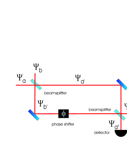
FIG. 1.: Principle of the Mach-Zehnder interferometer. Modes $\Psi_{a}$ and $\Psi_{b}$ are superposed on the first beamsplitter. After the beamsplitter has acted the modes $\Psi_{a^{\prime}}$, $\Psi_{b^{\prime}}$ are propagated along separate paths to a second beamsplitter. Mode $\Psi_{b^{\prime}}$ may undergo a variable phase shift induced by the phase shifter $\phi$. Modes $\Psi_{a^{\prime\prime}}$ and $\Psi_{b^{\prime\prime}}$ emerge after the second beamsplitter and one of the modes is put onto a detector. Varying $\phi$ will lead to a sinusoidal behavior of the intensity on the detector (fringes).

FIG. 2.: Interference fringes for simulated interferometers (a) of order $n=1$, (integration time per data point was 0.50 s); (b) $n=2$, (0.53 s) and (c) $n=3$, (0.63 s). $\langle n_{a^{\prime\prime}}\rangle$ is the probability to find the ion in $|1\rangle_{a^{\prime\prime}}$, while $t$ is the time for which the trap frequency was shifted by $\Delta\omega_{z}$, directly proportional to the phase shift $\phi=\Delta\omega_{z}~{}t$. The frequency of the fringes increases linearly with order $n$. $C$ is the observed contrast of the fringes.

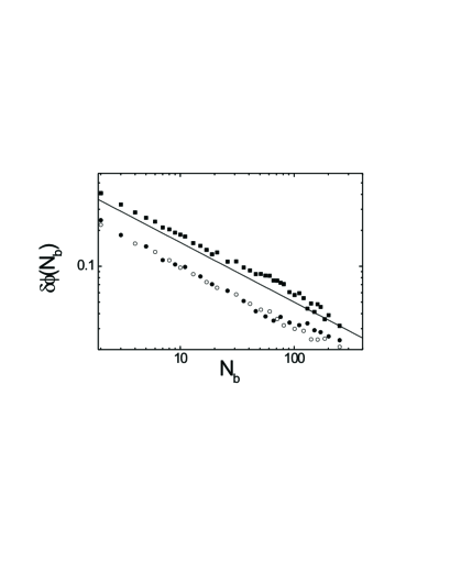
FIG. 3.: Noise-to-signal ratios $\delta\phi(N_{b})$ for the $n=1$ linear interferometer (solid squares), $n=2$ nonlinear interferometer (solid circles) and $n=3$ nonlinear interferometer (open circles) vs. the number of measurements $N_{b}$. The solid line is the theoretical limit for the linear (n=1) interferometer, assuming perfect contrast and detection efficiency.

REFERENCES

- [1] R. P. Feynman, Int. J. Theor. Phys. 21, 467 (1985).
- [2] S. Lloyd, Science 273, 1073 (1996).
- [3] S. Lloyd, and S. L. Braunstein, Phys. Rev. Lett. 82, 1784 (1999).
- [4] S. Somaroo et al., Phys. Rev. Lett. 82, 5381 (1999).
- [5] C. M. Caves, Phys. Rev. Lett. 45, 75 (1980).
- [6] C. M. Caves, Phys. Rev. D 23, 1693 (1981).
- [7] B. Yurke, S. L. McCall, and J. R. Klauder, Phys. Rev. A 33, 4033 (1986).
- [8] M. J Holland and K. Burnett, Phys. Rev. Lett. 71, 1355 (1995).
- [9] M. Xiao, L.-A. Wu, and H. J. Kimble, Phys. Rev. Lett. 59, 278 (1987).
- [10] for an overview see for example W. Tittel, and G. Weihs, Quant. Int. Comp. 1, 3 (2001).
- [11] A. Lamas-Linares, J. C. Howell, and D. Bouwmeester, Nature 412, 887 (2001); J. C. Howell, A. Lamas-Linares, and D. Bouwmeester, Phys. Rev. Lett. 88, 030401 (2002).
- [12] C. K. Law and J. H. Eberly, Phys. Rev. Lett. 76, 1055 (1996).
- [13] A. Ben-Kish et al., quant-ph/0208181 (2002).
- [14] D. J. Wineland et al., J. Res. Natl. Inst. Stand. Technol. 103, 259 (1998).
- [15] D. J. Wineland et al., Phys. Scr. T 76, 147 (1998).
- [16] For an extension of this class of Hamiltonians outside the Lamb-Dicke limit see R. L. de Matos Filho and W. Vogel, Phys. Rev. A 58, R1661 (1998).
- [17] The coupling can be experimentally arranged to depend or not depend on the internal state, see [14].
- [18] Note that Eq.(1) in [3] has a sign error in the right-hand side exponent.
- [19] D. M. Meekhof et al., Phys. Rev. Lett 76, 1796 (1996).
- [20] D. Leibfried et al., J. Mod. Opt. 44, 2485 (1997).
- [21] and both scale as , and differ only by in the Raman-detuning. Therefore sucessful impementation of implies the feasibility of .
- [22] C. A. Sackett, Quant. Inf. Comp. 1, 57 (2001).
- [23] M Rowe et al., Quant. Inf. Comp., 4, 257 (2002).
- [24] D. W. Allan, Proc. IEEE 54, 221 (1966).
- [25] W. M. Itano et al., Phys. Rev. A 47, 3554 (1993).