A measurement-based approach to quantum arrival times

Abstract

For a quantum-mechanically spread-out particle we investigate a method for determining its arrival time at a specific location. The procedure is based on the emission of a first photon from a two-level system moving into a laser-illuminated region. The resulting temporal distribution is explicitly calculated for the one-dimensional case and compared with axiomatically proposed expressions. As a main result we show that by means of a deconvolution one obtains the well known quantum mechanical probability flux of the particle at the location as a limiting distribution.

I Introduction

An important open problem in quantum theory is the question of how to formulate the notion of “arrival time” of a particle, such as an atom, at a given location, i.e. the time instant of its first detection there. This is clearly a very physical question, but when the extension and spreading of the wave packet is taken into account, a satisfactory formulation is far from obvious. The problem of time in quantum mechanics, both for time instants and time durations such as dwell time, has received a great deal of theoretical attention recently ML00 ; MSE02 . When the translational motion of the particle can be treated classically, a full quantum analysis of arrival time is in fact not necessary. This is the case for fast particles, and therefore arrival times are presently measured mostly by means of time-of-flight techniques, whose analysis is carried out in terms of classical mechanics. Problems, though, arise for slow particles for which the finite extent of the wavefunction and its spreading become relevant, such as for cooled atoms dropping out of a trap. Then a quantum theoretical point of view is needed. It is therefore important to find out when the classical approximations fail and to propose measurement procedures for arrival times in the quantum case. Since the theoretical definition of a quantum arrival time is still subject to debate it is necessary to determine what exactly such measurement procedures are measuring and to compare such operational approaches with the existing, more abstract and axiomatic, theories.

A simple one-dimensional example is the arrival time at $x=0$ of a particle described by a wave packet moving to the right. The probability of finding it still on the left side at time $t$ is $\int_{-\infty}^{0}dx|\psi(x,t)|^{2}$. Then it would seem natural to assume that the probability of arrival in $dt$ is given by the decrease in $dt$ of this integral, i.e. that the arrival-time probability density is its negative derivative. Since $\dot{\rho}+dJ_{\psi}/dx=0$, where $J_{\psi}$ is the usual quantum mechanical probability current, one immediately finds that the arrival-time probability density should be given by $J_{\psi}(0,t)$. For an ensemble of classical particles the arrival time distribution is also given by the flux, so everything seems to fit nicely. However, the quantum flux for a wavefunction formed entirely of positive-momentum components may become negative at certain times backflow . As a way out Leavens Leavens has proposed, following a Bohm trajectory analysis, to use its normalized absolute value.

The difficulties to formulate a quantum arrival time concept were posed most prominently by Allcock Allcock , and there are several attempts to overcome these ML00 ; BEM01d . Kijowski Kijowski74 , in particular, obtained a time-of-arrival distribution for free motion from a set of axioms modeled after the classical case; for a general investigation see Werner Werner . The distribution of Ref. Kijowski74 has been studied, compared to other approaches, and generalized by some of us for systems subject to interaction potentials and to multi-particle systems MLP98 ; MPL99 ; BSPME00 ; BEMS00 ; BEM01a ; BEM01b .

No procedure how to measure the proposed distributions was given, nor is one known today. The gap between experiment and axiomatically defined quantities has been commented on and considered to be worrying by Wigner and others; for a review see Ref. ML00 . In this vein, several “toy models” for arrival-time measurements have been put forward by Aharonov, Oppenheim, Reznik, Popescu and Unruh AOPRU98 (cf. also ML00 ; BEM01c ), but these models do not incorporate the basic irreversibility inherent in any measurement process. Irreversibility has been included by Halliwell Halliwell98b in a model based on a two-level detector in which the initial excited level decays due to the presence of the particle. However, the model remains somewhat abstract since no connection is made with any specific measuring system.

An experimentally very natural approach to determine the arrival time of an atom is by quantum optical means. A region of space may be illuminated by a laser and upon entering the region an atom will start emitting photons. The first photon emission can be taken as a measure of the arrival time of the atom in that region. This approach has been proposed by three of us and Baute MBDE00 , and in a preliminary study of the one-dimensional case a surprisingly good numerical agreement with Kijowski’s axiomatic distribution was found in some special examples.

From a fundamental point of view, however, immediate objections may be raised to this experimental, or operational, approach. First, depending on the decay rate of the excited atomic level, the photon emission will not be instantaneous but will take some time, thus leading to a delay compared to some “ideal” arrival time of the atom. Second, the laser takes some time to pump the atom from its ground-state to an excited state, and therefore this also leads to a delay. Conceivably, the second objection might be overcome by progressively increasing the laser intensity, and the first objection by considering shorter life times so that in a theoretical limit one would arrive at an “ideal” quantum arrival time without the above shortcomings. Attractive though this seems at first sight, it does not work, as will be shown in this paper. The reason is a further difficulty – reflection. Although the laser couples only to the internal degrees of the atom, it will be seen that there is a nonzero probability for the atom to be reflected from the laser region without ever emitting a photon. Nevertheless, there is a way out of these difficulties, with a surprising result. The idea is to “subtract” the delays from the first-photon probability density by means of a deconvolution with an atom at rest. This results in a distribution which, for shorter and shorter life time of the atomic level, converges to an unexpected distribution  –  namely to $J_{\psi}$, the quantum mechanical probability flux. The probability distribution for the first photon is non-negative and the emergence of possible small negative values is due to the deconvolution procedure. This connection to $J_{\psi}$ opens a way, to our knowledge for the first time, to measure the quantum mechanical probability flux.

For simplicity, this paper considers only the one-dimensional case. The probability density for the emission of the first photon from a moving atom is calculated explicitly by means of the quantum jump approach Hegerfeldt93 . It is shown that large laser intensities lead to a large reflection probability. This in turn leads to a large non-emission probability and a first-photon probability density not normalized to 1. Then the problem of reflection versus time delay is discussed. Reducing the laser intensity leads to a pumping delay. It is shown that trying to reduce the emission delay by shortening the level lifetime leads in the limit to a free wave packet in the ground-state with no emissions. The delays are then removed by a deconvolution, and we discuss for which parameters the resulting expression is close to its “ideal” limit $J_{\psi}$. For more practical purposes it is also shown that for a certain domain of parameters, which include those used in Ref. MBDE00 , the non-deconvoluted first-photon probability density gives a good approximation to $J_{\psi}$ and to Kijowski’s axiomatic arrival time distribution. However, it is also pointed out that Kijowski’s distribution cannot be obtained in a simple direct way as an exact limit of our operational approach.

II The probability density for the first photon

The Hamiltonian of a two-level atom of mass $m$, interacting with the quantized electromagnetic field ${\bf E}$ and a laser with (classical) field ${\bf E_{L}}$ is, in the usual dipole approximation and in the Schrödinger picture,

$$H=\frac{{\bf{\hat{p}}}^{2}}{2m}+H_{A}+H_{F}+e{{\bf D}}\cdot\left({\bf{E}}+{\bf E}_{L}\right)$$ (1)

where

$${}H_{A} = \frac{1}{2}\hbar\omega\left\{|2\rangle\langle 2|-|1\rangle\langle 1|\right\}$$ (2)

$$H_{F} = \sum_{\bf{k}\lambda}\hbar\omega_{\bf{k}}\hat{a}_{\bf{k}\lambda}^{\dagger}\hat{a}_{{\bf k}\lambda}$$

$${{\bf D}} = {\bf d}_{12}|1\rangle\langle 2|+{\rm h.c.}$$

with ${\bf d}_{12}$ the transition dipole moment between the states $|1\rangle$ and $|2\rangle$. It is assumed that the laser illuminates a half space, $x_{1}\geq 0$, say.

Let an atomic state $|\Psi(t_{0})\rangle$ be prepared at time $t_{0}$. By means of the quantum jump approach Hegerfeldt93 the atomic time development until the first photon detection is given by a (non-hermitean) “conditional” Hamiltonian $H_{\rm c}$,

$$|\Psi(t)\rangle=e^{-iH_{\rm c}(t-t_{0})/\hbar}|\Psi(t_{0})\rangle,$$ (3)

with the photon part traced away. In the interaction picture with respect to the internal Hamiltonian $H_{A}$ one has in the usual rotating wave approximation

$$H_{\rm c}={\bf{\hat{p}}}^{2}/2m+\frac{\hbar}{2}\Omega\,\Theta(\hat{x}_{1})\left\{|2\rangle\langle 1|e^{i{\bf k}_{L}\cdot{\hat{\bf x}}}+{\rm h.c.}\right\}-\frac{i}{2}\hbar\gamma|2\rangle\langle 2|~{},$$ (4)

where the Rabi frequency $\Omega\propto{\bf d}\cdot{\bf E}^{(0)}_{L}$ plays the role of a laser-atom coupling constant (with ${\bf E}^{(0)}_{L}$ the laser amplitude), ${\bf k}_{L}$ is the laser wave vector, and where $\gamma$ is the Einstein coefficient of level 2, i.e. its decay rate or inverse life time. One can show that Eq. (4) includes the Doppler effect, i.e. the laser driving depends on the atomic velocity through a frequency shift. The probability, $N_{t}$, of no photon detection from $t_{0}$ up to time $t$ is given by Hegerfeldt93

$$N_{t}=||e^{-iH_{\rm c}(t-t_{0})/\hbar}|\psi(t_{0})\rangle||^{2},$$ (5)

and the probability density, $\Pi(t)$, for the first photon detection by

$$\Pi(t)=-\frac{dN_{t}}{dt}.$$ (6)

For simplicity, we only consider the corresponding one-dimensional problem, with the laser perpendicular to the atomic motion, so that the Doppler effect plays no role. With $|1\rangle\equiv{1\choose 0}$ and $|2\rangle\equiv{0\choose 1}$ the conditional Hamiltonian becomes, in matrix form

$$H_{\rm c}=\hat{p}^{2}/2m+\frac{\hbar}{2}\left({0\atop 0}{0\atop-i\gamma}\right)+\frac{\hbar}{2}\,\Theta(\hat{x})\left({0\atop\Omega}{\Omega\atop 0}\right).$$ (7)

To obtain the time development of a general wave packet under $H_{\rm c}$ we first solve the eigenvalue equation

$$H_{\rm c}{\bf\Phi}=E{\bf\Phi},~{}~{}~{}~{}~{}{\rm where}~{}~{}{\bf\Phi}(x)\equiv{\phi^{(1)}(x)\choose\phi^{(2)}(x)}.$$ (8)

Since for $x<0$ there is no laser one obtains for $\phi^{(i)}$ the equations

$$\frac{\hat{p}^{2}}{2m}\phi^{(1)}=E\phi^{(1)},~{}~{}~{}(\frac{\hat{p}^{2}}{2m}-i\hbar\gamma/2)\phi^{(2)}=E\phi^{(2)}.$$ (9)

Hence $\phi^{(1)}$ is a combination of $e^{ikx}$ and $e^{-ikx}$ with $k$ satisfying

$$E=\hbar^{2}k^{2}/2m\equiv E_{k}$$ (10)

while $\phi^{(2)}$ is a combination of $e^{iqx}$ and $e^{-iqx}$ with $q$ satisfying

$$E+i\hbar\gamma/2=\hbar^{2}q^{2}/2m~{}.$$ (11)

We now look for eigenstates of $H_{\rm c}$ which correspond to a ground-state plane wave coming in from the left. Then $k$ as well as $E$ must be real, by boundedness, and for $x\leq 0$ the eigenstate is of the form

$${\bf\Phi}_{k}(x)=\frac{1}{\sqrt{2\pi}}\left({e^{ikx}+R_{1}e^{-ikx}\atop R_{2}e^{-iqx}}\right),\quad x\leq 0,\quad k>0,$$ (12)

with ${\rm Im}\,q>0$ for boundedness, while $R_{1}$ and $R_{2}$ are reflection amplitudes yet to be determined. Note that although $E=E_{k}$ is real the complete wave functions will not be orthogonal, in accordance with the non-hermiticity of $H_{\rm c}$.

To obtain the form of ${\bf\Phi}_{k}(x)$ for $x>0$ we denote by $|\lambda_{+}\rangle$ and $|\lambda_{-}\rangle$ the eigenstates of the matrix $\frac{1}{2}\left({0\atop\Omega}{\Omega\atop-i\gamma}\right)$ corresponding to the eigenvalues $\lambda_{\pm}$. One easily finds

$$\lambda_{\pm} = -\frac{i}{4}\gamma\pm\frac{i}{4}\sqrt{\gamma^{2}-4\Omega^{2}}$$ (13)

$$|\lambda_{\pm}\rangle = {1\choose 2\lambda_{\pm}/\Omega}~{}.$$ (14)

We exclude, for the moment, the limiting case $\lambda_{+}=\lambda_{-}$. Note that $|\lambda_{\pm}\rangle$ are not orthogonal and have not been normalized. For $x\geq 0$, one can write ${\bf\Phi}_{k}$ as a superposition of $|\lambda_{\pm}\rangle$ in the form

$$\sqrt{2\pi}{\bf\Phi}_{k}(x)=C_{+}|\lambda_{+}\rangle e^{ik_{+}x}+C_{-}|\lambda_{-}\rangle e^{ik_{-}x},\qquad x\geq 0.$$ (15)

From the eigenvalue equation $H_{\rm c}{\bf\Phi}_{k}=E_{k}{\bf\Phi}_{k}$, together with $E_{k}=\hbar^{2}k^{2}/2m$, one obtains for $x\geq 0$

$$k_{\pm}^{2}=k^{2}-2m\lambda_{\pm}/\hbar=k^{2}+im\gamma/2\hbar\mp im\sqrt{\gamma^{2}-4\Omega^{2}}/2\hbar,$$

with Im$\,k_{\pm}>0$ for boundedness. From the continuity of ${\bf\Phi}_{k}(x)$ at $x=0$ one gets, with $|1\rangle={1\choose 0}$ and $|2\rangle={0\choose 1}$,

$$1+R_{1} = C_{+}\langle 1|\lambda_{+}\rangle+C_{-}\langle 1|\lambda_{-}\rangle$$

$$R_{2} = C_{+}\langle 2|\lambda_{+}\rangle+C_{-}\langle 2|\lambda_{-}\rangle.$$

Similar relations result from the continuity of ${\bf\Phi}_{k}^{\prime}(x)$ at $x=0$, yielding

$$C_{+} = -{2k(q+k_{-})\lambda_{-}}/D,$$ (16)

$$C_{-} = 2k(q+k_{+})\lambda_{+}/D,$$

$$R_{2} = k(k_{-}-k_{+})\Omega/D,$$

$$R_{1} = [\lambda_{+}(q+k_{+})(k-k_{-})-\lambda_{-}(q+k_{-})(k-k_{+})]/D,$$

where the common denominator $D$ is given by

$$D=(k+k_{-})(q+k_{+})\lambda_{+}-(k+k_{+})(q+k_{-})\lambda_{-}\,.$$ (17)

Thus Eq. (15) becomes, in components and for $x\geq 0$,

$$\phi_{k}^{(1)}(x) = -\frac{2k}{\sqrt{2\pi}D}\left\{(q+k_{-})\lambda_{-}e^{ik_{+}x}-(q+k_{+})\lambda_{+}e^{ik_{-}x}\right\},$$ (18)

$$\phi_{k}^{(2)}(x) = \frac{k\Omega}{\sqrt{2\pi}D}\left\{(q+k_{-})e^{ik_{+}x}-(q+k_{+})e^{ik_{-}x}\right\}.$$

The case $\lambda_{-}=\lambda_{+}$ is obtained from this by taking limits. For later purposes we also consider increasingly large $\gamma$, the other parameters kept fixed. This leads to

$$\lambda_{+} \approx -i\Omega^{2}/2\gamma\to 0,$$ (19)

$$\lambda_{-} \approx -i\gamma/2+i\Omega^{2}/2\gamma\to-i\gamma/2,$$ (20)

$$k_{+}^{2} \approx k^{2}+im\Omega^{2}/\hbar\gamma,\quad\quad k_{+}\to k,$$ (21)

$$k_{-}^{2} \approx k^{2}+im\gamma/\hbar\approx im\gamma/\hbar,$$ (22)

$$q \approx \left\{im\gamma/\hbar\right\}^{1/2},$$ (23)

$$C_{-}, \!\!\!\!\!\!\!\!\!R_{1},\,R_{2}\to 0,$$ (25)

$$C_{+}\to 1.$$

In this case the state vector for $x>0$ becomes simply the plane wave with wave number $k$ in the ground state. This means that for increasing $\gamma$ there is less and less reflection, but also less and less absorption, i.e. photon detection, so that the laser has less and less effect on the atom.

At first sight the occurrence of reflections may seem surprising since the laser only couples to the internal degrees of the atom and since $H_{\rm c}$ only applies to the time development before the first photon detection. Physically this can be understood from the coupling of the atom to the quantized electromagnetic field. The laser changes the internal state, this in turn changes the quantized electromagnetic field and its momentum distribution. This in turn changes the momentum distribution of the atomic motion. Mathematically the reason is of course the step function in front of the matrix, similar as for a square-well potential. The consequences of the nonzero reflection will be discussed further below.

By decomposing an initial state as a superposition of eigenfunctions one obtains its conditional time development. This is easy for an initial ground-state wave packet ${\psi(x,t_{0})\choose 0}$ coming in from the far left side and with $t_{0}$ in the remote past. Indeed, if $\widetilde{\psi}(k)$ denotes the momentum amplitude the wave packet would have as a freely moving packet at $t=0$, then

$${\bf\Psi}(x,t)=\int_{0}^{\infty}dk\,\widetilde{\psi}(k)\,{\bf\Phi}_{k}(x)\,e^{-i\hbar k^{2}t/2m}$$ (26)

describes the conditional time development of a state which in the remote past behaves like a wave packet in the ground-state coming in from the left.

III The reflection problem and the no-detection probability

From Eq. (5) one obtains, with ${\bf\Psi}={\psi^{(1)}\choose\psi^{(2)}}$,

$$N_{t}=\int dx\{|\psi^{(1)}(x,t)|^{2}+|\psi^{(2)}({\bf x},t)|^{2}\}$$ (27)

and Eq. (6) becomes

$$\Pi(t)=\frac{i}{\hbar}\langle\psi(t)|H_{\rm c}-H_{\rm c}^{\dagger}|\psi(t)\rangle.$$ (28)

Since $H_{\rm c}-H_{\rm c}^{\dagger}=-i\gamma\hbar|2\rangle\langle 2|$, the first-photon probability density is given by

$$\Pi(t)=\gamma\int_{-\infty}^{\infty}dx\,|\psi^{(2)}(x,t)|^{2}.$$ (29)

The probability of no photon detection at all is, for $t_{0}$ in the remote past,

$$1-\int_{-\infty}^{\infty}dt^{\prime}\,\Pi(t^{\prime})=N_{t=\infty}.$$ (30)

For physical reasons, only $\psi^{(1)}$ contributes to this, and only for $x<0$. The latter follows from the fact that, for $x>0$, the ground-state part will eventually be pumped by the laser to the excited state. Since $t=\infty$ in Eq. (30), only the reflected part remains, and hence the no-detection probability becomes

$$N_{t=\infty}=\int_{0}^{\infty}dk\,|R_{1}(k)|^{2}|\widetilde{\psi}(k)|^{2}.$$ (31)

As a consequence, $\Pi(t)$ is in general not normalized to $1$. Physically the probability for missing an atom increases with $\Omega$, the strength of the laser driving. This is also seen mathematically from the expression for $R_{1}$ in Eq. (16). An example is given in Section V (cf. Fig. 4 further below) and a practical approach to bypass this problem is also discussed there.

On the other hand, for $k\rightarrow\infty$ reflection becomes negligible since then $R_{i}\rightarrow 0$. Hence for faster atoms reflection does not pose a problem. This will also be exploited for practical purposes in Section V.

IV Delays versus reflections and an idealized distribution

The approach to quantum arrival times by means of first-photon detections contains a built-in “delay” since an excited atom will not emit a photon immediately, due to the finite decay rate $\gamma$. This is in addition to the time the photon takes to reach the detector; the photon travel time, however, can easily be taken into account, so it will not be considered here any further.

It seems natural to try to obtain an ideal arrival-time distribution by considering faster and faster decay times, i.e. taking $\gamma\rightarrow\infty$, at least theoretically. This will not work, however. The reason is that for increasing $\gamma$, with all other parameters kept fixed, the driving by the laser becomes less efficient so that, in the limit $\gamma\rightarrow\infty$, the wave packet remains unaffected, with no excitation and no reflection, as can be seen from Eqs. (19) - (25) above. Moreover, if both $\gamma$ and $\Omega$ go to infinity with $\gamma/\Omega$ kept fixed, then $R_{1}\to-1$ and everything is completely reflected without excitation repulsion .

One might also be tempted to avoid reflection by choosing weak driving, $\Omega/\gamma\ll 1$. This, however, would cause a severe delay problem since the laser would take more time to pump the atom to the excited state. Hence the first-photon emission would also take more time. To see how relevant detection delays are, we have compared $\Pi(t)$ with the flux $J_{\psi}$ and the axiomatic probability distribution $\Pi_{\rm K}(t)$ of Kijowski for a Gaussian wave packet. The result is given in Fig. 1.

Figure 1: Time-of-arrival distributions: Flux $J$ (solid line, here indistinguishable from Kijowski’s $\Pi_{K}$) and $\Pi$ (first photon, dots). Note the delay in $\Pi$. The initial state is a minimum-uncertainty-product Gaussian for the center-of-mass motion of a single Cesium atom in the ground state with $\langle v\rangle=9.0297$ cm/s, $\langle x\rangle=-1.85$ $\mu$m, and $\Delta x=0.26$ $\mu$m.; $\Omega=0.0999\gamma$; all figures are for the transition $6^{2}P_{3/2}$ – $6^{2}S_{1/2}$ of Cesium with $\gamma=33.3$ MHz.

Depending on the parameters, the delay and reflection problem may be either very relevant or negligible. A detailed analytic investigation of this question is given in Section V.

A way out of the conflicting problems of reflection (missed atom) and increasing delay times for weaker driving is the transition from the “experimental” $\Pi(t)$ to an idealized arrival-time distribution, obtained as follows. A two-level atom at rest, when driven by a resonant laser, has a definite probability density, $W(t)$, for the detection of the first photon, given by 2level

$$W(t)=\frac{\gamma\Omega^{2}}{4|S|^{2}}e^{-\gamma t/2}|e^{St/2}-e^{-St/2}|^{2}\Theta(t),$$ (32)

with

$$S=\frac{1}{2}(\gamma^{2}-4\Omega^{2})^{1/2}.$$

Intuitively, the delay-time mechanism for a moving atom ought to be similar to that for an atom at rest. Should it then not be possible to somehow compensate the delay in $\Pi(t)$ by that of the atom at rest and thus arrive, in some limit, at a delay-free ideal distribution? To achieve this, we assume the (experimental) arrival-time distribution $\Pi(t)$ to be the convolution of a hypothetical ideal distribution, $\Pi_{\rm id}$, with the distribution $W(t)$ for an atom at rest,

$$\Pi=\Pi_{\rm id}*W.$$ (33)

The delay in $\Pi$ is then mainly due to that contained in $W$.

The hypothetical ideal distribution $\Pi_{\rm id}$ is obtained by a deconvolution via Fourier transform from $\widetilde{\Pi}_{\rm id}=\widetilde{\Pi}/\widetilde{W}$ where ${\widetilde{\Pi}}(\nu)=\int dte^{-i\nu t}\Pi(t)$ etc. From Eqs. (29) and (26) one finds

$${\widetilde{\Pi}}(\nu)=\gamma\int dx\int dk\int dk^{\prime}\,\overline{{\widetilde{\psi}}(k)}{\widetilde{\psi}}(k^{\prime})\overline{\phi_{k}^{(2)}(x)}\phi^{(2)}_{k^{\prime}}(x)2\pi\delta\left(\nu-\frac{\hbar}{2m}(k^{2}-k^{\prime 2})\right)$$ (34)

and from Eq. (32)

$$\widetilde{W}(\nu)=\frac{\Omega^{2}\gamma/2}{\left\{\left(i\nu+\gamma/2\right)^{2}-S^{2}\right\}\left\{i\nu+\gamma/2\right\}},$$ (35)

and thus

$$\frac{1}{\widetilde{W}(\nu)}=1+C_{1}i\nu+C_{2}(i\nu)^{2}+C_{3}(i\nu)^{3},$$ (36)

where

$$C_{1}=\left(\frac{\gamma}{\Omega^{2}}+\frac{2}{\gamma}\right),\quad C_{2}=\frac{3}{\Omega^{2}}~{},\quad C_{3}=\frac{2}{\gamma\Omega^{2}}~{}.$$ (37)

In the time domain this gives

$$\Pi_{\rm id}(t)=\Pi(t)+C_{1}\Pi^{\prime}(t)+C_{2}\Pi^{\prime\prime}(t)+C_{3}\Pi^{\prime\prime\prime}(t)~{}.$$ (38)

In the limit of no reflection, for $\gamma\rightarrow\infty$, the delay problem pointed out above for $\Pi$ should be absent for $\Pi_{\rm id}$. In fact, in this limit one sees from Eqs. (19) - (23) and from Eq. (36) that in $1/{\widetilde{W}}$ only $i\nu\gamma/\Omega^{2}$ remains relevant for large $\gamma$. Furthermore, $R_{2}\to 0$ for $\gamma\rightarrow\infty$, and since $e^{-iqx}\rightarrow 0$ in Eq. (34) the integral over $x\leq 0$ goes to zero. Similarly the terms in $\phi^{(2)}_{k}(x)$ and $\phi^{(2)}_{k^{\prime}}(x)$ containing $e^{-i\bar{k}_{-}x}$ and $e^{ik^{\prime}_{-}x}$ drop out. For $\gamma\rightarrow\infty$ one has, from Eqs. (19) and (25), $C_{+}\rightarrow 1$ and the integration of $\exp\{-i\bar{k}_{+}x+ik^{\prime}_{+}x\}$ over $x\geq 0$ gives $i/(k^{\prime}_{+}-\bar{k}_{+})$. Hence

$$\frac{\widetilde{\Pi}(\nu)}{\widetilde{W}(\nu)}\rightarrow\frac{4\gamma}{2\pi}\int dkdk^{\prime}\overline{{\widetilde{\psi}}(k)}\widetilde{\psi}(k^{\prime})\frac{\bar{\lambda}_{+}\lambda_{+}}{\Omega^{2}}\frac{i}{k_{+}^{\prime}-\bar{k}_{+}}\frac{i\nu\gamma}{\Omega^{2}}2\pi\delta\left(\nu-\frac{\hbar}{2m}(k^{2}-k^{\prime 2})\right).$$ (39)

By the $\delta$ function, $\nu=\hbar(k-k^{\prime})(k+k^{\prime})/2m$. Hence in the limit $\gamma\rightarrow\infty$ one obtains, by Eqs. (19) - (23),

$$\frac{\widetilde{\Pi}(\nu)}{\widetilde{W}(\nu)}\rightarrow\frac{1}{2\pi}\frac{\hbar}{2m}\int dkdk^{\prime}\overline{\widetilde{\psi}(k)}{\widetilde{\psi}}(k^{\prime})(k+k^{\prime})2\pi\delta\left(\nu-\frac{\hbar}{2m}(k^{2}-k^{\prime 2})\right).$$ (40)

Going to the time domain one finally obtains

$$\Pi_{\rm id}(t) \rightarrow \frac{1}{2\pi}\frac{\hbar}{m}\int dkdk^{\prime}\overline{\widetilde{\psi}(k)}e^{i\hbar k^{2}t/2m}\frac{k+k^{\prime}}{2}{\widetilde{\psi}}(k^{\prime})e^{-i\hbar k^{\prime 2}t/2m}$$

$$= \frac{\hbar}{2mi}\left\{\overline{\psi(0,t)}\psi^{\prime}(0,t)-\overline{\psi^{\prime}(0,t)}\psi(0,t)\right\},$$

which is the flux $J_{\psi}$ for the free wavefunction $\psi(x,t)$ at $x=0$, i.e. without laser footnote1 .

This is an extremely interesting result since $J_{\psi}$ is a natural candidate for the arrival-time distribution, as pointed out in the Introduction. We note that $J_{\psi}$ is normalized to 1 for a particle which has only positive momentum components. This is seen for example from Eq. (40) for $\nu=0$.

The limit in Eq. (IV) means that $\Pi_{\rm id}$ can be approximated by $J_{\psi}$ for sufficiently large $\gamma$. Physically, it is important to determine the parameter ranges for which this approximation is a good one. For this to be valid a simple sufficient condition on the parameters can be derived as follows. First one considers the case $\Omega^{2}/\gamma^{2}\ll 1$ (weak driving) and makes the corresponding approximations in $\Pi_{\rm id}(t)$. Denoting by $\Delta E$ a measure of the magnitude of

$$\frac{\hbar^{2}}{2m}|k^{2}-k^{\prime 2}|\,,$$ (42)

as determined by $\widetilde{\psi}(k)$ and $\widetilde{\psi}(k^{\prime})$, one then considers the case $\gamma\gg\Delta E/\hbar$ and $\Delta E/\hbar\gg\Omega^{2}/\gamma$. Then one obtains that $\Pi_{\rm id}$ is close to $J_{\psi}$. The inequalities can be written in the form

$$\Omega^{2}/\gamma\ll\Delta E/\hbar\ll\gamma$$ (43)

Thus $\Pi_{\rm id}$ can be replaced by $J_{\psi}$ if these inequalities are satisfied. Even outside this parameter range, $J_{\psi}$ may be an excellent approximation to $\Pi_{\rm id}$, as shown in Fig. 2. The convergence of $\Pi_{\rm id}$ to $J_{\psi}$ shows that also $\Pi_{\rm id}$ may contain small negative values. Since this occurs neither for $\Pi$ nor for $W$, the intuitive ansatz of Eq. (33) cannot always be fulfilled with a strictly positive distribution. The reason for this clearly is that the ansatz of a convolution in Eq. (33) is too simple and ought to be replaced by something more sophisticated. On the other other hand, this result gives a handle at the quantum mechanical probability flux and indicates a method how to measure it.

The above deconvolution procedure which recovers the quantum mechanical particle flux essentially works because the weak-excitation limit taken allows a clear separation of (1) the time dependence associated with the motion of the wavepacket, and (2) the time dependence associated with the internal degrees of freedom (excitation, Rabi oscillation, and decay). It seems reasonable that this might be done. However, the weak-excitation limit implies that the waiting times for the first scattered photon are of the order $\gamma/\Omega^{2}$ and therefore very long. Hence the number to be measured is essentially to be obtained from the subtraction of two very large numbers. Experimentally this is a difficult thing to do with high accuracy and requires small measurement errors. For practical purposes it is therefore important to know when delays and reflections can be safely neglected, since then the transition to $\Pi_{\rm id}$ by deconvolution is not necessary. This is investigated quantitatively in the next section.

Figure 2: Excellent agreement between $\Pi_{\rm id}$ (filled circles) and $J$ (solid line); deviations from $\Pi_{K}$ (dotted line) and $\Pi$ (dot-dashed line). The initial wave packet is a coherent combination $\psi=2^{-1/2}(\psi_{1}+\psi_{2})$ of two Gaussian states for the center-of-mass motion of a single Cesium atom that become separately minimal uncertainty packets (with $\Delta x_{1}=\Delta x_{2}=0.021\,\mu$m, and average velocities $\langle v\rangle_{1}=18.96$ cm/s, $\langle v\rangle_{2}=5.42$ cm/s) at $x=0$ and $t=2\,\,\mu$s; $\Omega=0.37\gamma$.

V Parameter ranges with negligible delay and reflection.

In the case of weak driving, $\Omega\ll\gamma$, the excited state population is negligible compared to that of the ground state. Hence the reflection coefficient for the ground state is the only one that matters in this case,

$$|R_{1}(k)|^{2}\approx\frac{1}{64}(\Omega/\gamma)^{2}(\hbar\Omega/E)^{2},$$ (44)

This is small if $E\gtrsim\hbar\Omega$. For strong driving, $\Omega\gg\gamma$, the reflection coefficients take a simple form when the energy E of the plane wave satisfies

$$E\gg\hbar\Omega.$$ (45)

Then both states are populated roughly equally for $x>0$, and with Eq. (45) the reflection coefficients become

$$|R_{1}(k)|^{2}\approx\frac{1}{32^{2}}(\hbar\Omega/E)^{4},\;\;\;|R_{2}(k)|^{2}\approx\frac{1}{64}(\hbar\Omega/E)^{2}.$$ (46)

Both coefficients are small if Eq. (45) holds.

To quantify the detection delay, let us define $\tau_{d}$ as the difference between the average time of the first photon emission, $\langle t\rangle_{\Pi}=\int_{-\infty}^{\infty}dt\,t\,\Pi(t)$, and $\langle t\rangle_{J}=\int_{-\infty}^{\infty}dt\,t\,J_{\psi}$ footnote2 ; we note that the “average arrival time” at $x=0$ evaluated with the flux at $x=0$, $\langle t\rangle_{J}$ coincides with the average of Kijowski’s distribution Kijowski74 ; ML00 . For negligible reflection, ${\bf\Psi}(x,t)$ is, for $x<0$, nearly the same as the free wavefunction, and therefore, by a partial integration,

$$\tau_{d}=\langle t\rangle_{\Pi}-\langle t\rangle_{J}=\int_{-\infty}^{\infty}dt\,N_{t}^{+}~{}~{}~{}~{}{\rm(for~{}negligible~{}reflection)},$$ (47)

where $N_{t}^{+}=\int_{0}^{\infty}(|\psi^{(1)}(x,t)|^{2}+|\psi^{(2)}(x,t)|^{2})\,dx$. Hence, in the case of negligible reflection the delay is associated with the amount of penetration of the wave into the laser region. For weak and strong driving a straightforward calculation yields the simple results

$$\tau_{d} \approx \gamma/\Omega^{2}\;\;{\rm(weak\;driving}).$$ (48)

$$\tau_{d} \approx 2/\gamma\;\;\,{\rm(strong\;driving),}$$ (49)

It is interesting to note, and physically very reasonable, that this coincides with the average time between two photon emissions for a two-level atom at rest, driven by a resonant laser, as easily seen from Eq. (32). If $\Delta t$ denotes the width of $\Pi(t)$, then one needs $\tau_{d}\ll\Delta t$ for the delay to be negligible.

If one denotes by $\widetilde{E}$ the average energy for wave packets that are sharply peaked in energy or, more generally, as the smallest significant energy component, then the above conditions for negligible reflection and negligible delay can be summarized as

$$\hbar/{\widetilde{E}}\lesssim\gamma/\Omega^{2} \ll \Delta t\;\;\;\;\;\;\;\;\;\;~{}~{}~{}~{}~{}~{}~{}~{}~{}({\rm weak\,\,driving})$$ (50)

$$\hbar/\widetilde{E}\ll\Omega^{-1} \ll 2/\gamma\ll\Delta t\;\;\;~{}~{}~{}~{}({\rm strong\,\,driving}).$$ (51)

Fig. 3 shows a striking example for which these conditions are fulfilled. Here the first-photon distribution $\Pi$ is indistinguishable from $J_{\psi}$ and from Kijowski’s distribution.

Figure 3: Negligible delay and reflection with Eq. (51): $\Pi$ (first photon, dots) and $J_{\psi}$ (solid line, here indistinguishable from $\Pi_{K}$) for initial Gaussian parameters $\langle v\rangle=90.30$ cm/s, $\langle x\rangle=-218.02$ $\mu$m, $\Delta x=26.46$ $\mu$m; $\Omega=5\gamma$.

For strong driving the delay due to the time needed for pumping the atom to an excited level is small, but on the other hand there is a large probability to miss out the atom altogether if the condition $E\gg\hbar\Omega$ is not fulfilled. As a consequence, the first-photon probability density $\Pi(t)$ will not be normalized to 1. Let us then define a normalized distribution $\Pi_{N}(t)=\Pi(t)/\int dt^{\prime}\,\Pi(t^{\prime})$. For practical purposes this can be amazingly efficient in some parameter domains as Fig. 4 shows. There, $\Pi$ is far from being normalized to 1, but $\Pi_{N}$ and $J_{\psi}$, which in this example has no negative parts, coincide beautifully. Interestingly, one notices a small difference to Kijowski’s distribution. It might also be possible to use the general normalization procedure in terms of operators proposed in Ref. BF01 .

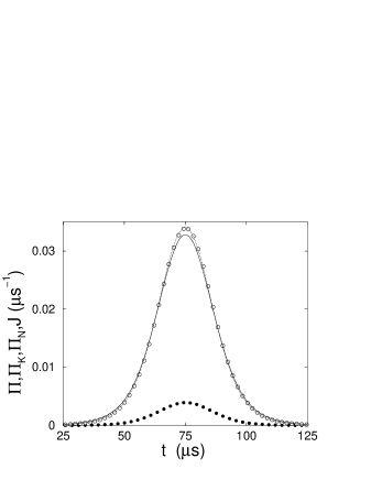
Figure 4: Improvement by normalization: $\Pi_{N}$ (white circles) right on top of $J_{\psi}$ (dashed line); also shown $\Pi_{K}$ (solid line) and $\Pi$ (filled circles). The initial Gaussian wave packet is chosen to become minimal when its center arrives at $x=0$ (in the absence of the laser) to enhance the difference between $\Pi_{K}$ and $J_{\psi}$; $\langle v\rangle=0.9$ cm/s, $\Delta x=0.106$ $\mu$m, $\Omega=3\gamma$.

VI Conclusions

In this paper, we have investigated a proposal to determine arrival times of quantum mechanical particles. The proposal is based on the intuitive idea to illuminate the arrival region by a laser and to consider a traveling two-level atom. The time of the first emitted photon is then taken as a measure for the arrival time. By repeating the experiment one obtains a probability density, $\Pi(t)$, for the time of the first photon. We have discussed for the one-dimensional case in what way $\Pi(t)$ can be regarded as an atomic arrival-time distribution. Restrictions arise from reflections and delays. Reflections originate from the interaction with the laser and delays from the time needed for the pumping and the ensuing photon emission. The natural idea that an ideal or an axiomatically proposed distribution might be obtained from $\Pi(t)$ in the limit of a very strong or very weak laser and very large Einstein decay coefficient of the excited level has turned out not to be true. However, and this is a main theoretical result of the paper, one can subtract the delay by a deconvolution with the first-photon probability density for an atom at rest and then, surprisingly, for larger and larger Einstein coefficient one obtains the quantum mechanical probability current $J$ as the limit distribution. This quantity $J$ has previously been considered on axiomatic grounds as a candidate for the arrival time distribution, and the connection of $\Pi(t)$ with $J$ indicates, to our knowledge for the first time, a way to measure the quantum mechanical probability flux. We have also determined parameter domains for which the deconvoluted expression is already sufficiently close to $J$. Although the non-deconvoluted $\Pi(t)$ is not the same as $J$ and the axiomatically proposed distribution of Kijowski, it can, for experimental purposes, approach the latter two sufficiently closely. Parameter domains for which this holds have been explicitly determined; this is another main result of the paper, more of a practical nature.

- (1) J. G. Muga and C. R. Leavens, Phys. Rep. 338, 353 (2000).
- (2) J. G. Muga, R. Sala and I. L. Egusquiza (eds.), Time in Quantum Mechanics (Springer, Berlin, 2002).
- (3) Up to 4% of the norm can go backwards, cf. A. J. Bracken and G. F. Melloy, J. Phys. A: Math. Gen. 27, 2197 (1994). For this backflow effect see also G. R. Allcock, Ann. Phys. (N.Y.) 53, 311 (1969) and J. G. Muga, J. P. Palao and C. R. Leavens, Phys. Lett. A 253, 21 (1999), quant-ph/9803097.
- (4) C. R. Leavens, Ref. MSE02 , Chap. 5.
- (5) G. R. Allcock, Ann. Phys. (N.Y.) 53, 253 (1969); 53, 286 (1969); 53, 311 (1969).
- (6) A. D. Baute, I. L. Egusquiza, and J. G. Muga, J. Phys. A 34, 4289 (2001), eprint quant-ph/0104043.
- (7) J. Kijowski, Rep. Math. Phys. 6, 361 (1974).
- (8) R. Werner, J. Math Phys. 27, 793 (1986)
- (9) J. G. Muga, R. Leavens, J. P. Palao, Phys. Rev. A 58, 4336 (1998).
- (10) J. G. Muga, J. P. Palao, and C. R. Leavens, Phys. Lett. A 253, 21 (1999), eprint quant-ph/9807066.
- (11) A. D. Baute, R. Sala Mayato, J. P. Palao, J. G. Muga and I. L. Egusquiza, Phys. Rev. 61, 022118 (2000), eprint quant-ph/9904055.
- (12) A. D. Baute, I. L. Egusquiza, J. G. Muga and R. Sala Mayato, Phys. Rev. A 61 052111 (2000), eprint quant-ph/9911088.
- (13) A. D. Baute, I. L. Egusquiza, and J. G. Muga, Phys. Rev. 64, 012501 (2001), eprint quant-ph/0102005.
- (14) A. D. Baute, I. L. Egusquiza, and J. G. Muga, Phys. Rev. A 65, 032114 (2002), eprint quant-ph/0109133.
- (15) Y. Aharonov, J. Oppenheim, S. Popescu, B. Reznik, and W. G. Unruh, Phys. Rev. A 57, 4130 (1998), eprint quant-ph/9709031.
- (16) A. D. Baute, I. L. Egusquiza, and J. G. Muga, Phys. Rev. A 64, 014101 (2001), eprint quant-ph/0012051.
- (17) J. J. Halliwell, Prog. Theor. Phys. 102, 707 (1999), eprint quant-ph/9805057.
- (18) J. G. Muga, A. D. Baute, J. A. Damborenea, I. L. Egusquiza, eprint quant-ph/0009111.
- (19) G. C. Hegerfeldt and T. S. Wilser, in: Classical and Quantum Systems. Proceedings of the Second International Wigner Symposium, July 1991, edited by H. D. Doebner, W. Scherer, and F. Schroeck, (World Scientific, Singapore, 1992), p. 104; G. C. Hegerfeldt, Phys. Rev. A 47, 449 (1993); G. C. Hegerfeldt and D.G. Sondermann, Quantum Semiclass. Opt. 8, 121 (1996). For a review cf. M. B. Plenio and P. L. Knight, Rev. Mod. Phys. 70, 101 (1998). The quantum jump approach is essentially equivalent to the Monte-Carlo wavefunction approach of J. Dalibard, , Y. Castin and K. Mølmer, Phys. Rev. Lett., 68, 580 (1992), and to the quantum trajectories of H. Carmichael, An Open Systems Approach to Quantum Optics, Lecture Notes in Physics m18, (Springer, Berlin, 1993).
- (20) More precisely, if and are of the same order of magnitude and or, alternatively, if and , then . Physically, both conditions mean that the distance traveled by the atom in the time it takes for a photon to be scattered is much less than the de Broglie wave length.
- (21) M. S. Kim, P. L. Knight, and K. Wodkiewicz, Opt. Commun. 62, 385 (1987)
- (22) For wavefunctions with positive momenta, Kijowski’s distribution is obtained by replacing with in Eq. (IV). The occurrence of a square root of shows that this distribution cannot be obtained from or in a simple direct way as a limiting case since the latter contain only integer powers of .
- (23) A similar analysis was carried out in J. G. Muga, S. Brouard and D. Macías, Annals of Physics 240, 351 (1995) for a simpler one-channel system with absorption.
- (24) R. Brunetti and K. Fredenhagen, eprint quant-ph/0103144