Classicality of spin coherent states via entanglement and distinguishability

Abstract

We trace the resistance to entanglement generation of spin coherent states when passed through a beam splitter as we vary $S$ through $S=1/2\rightarrow\infty$. In the infinite $S$ limit the spin coherent states are equivalent to the high-amplitude limit of the optical coherent states. These states generate no entanglement and are completely distinguishable. This transition is discussed in terms of the classicality of the states. The decline of the generated entanglement, and in this sense increase in classicality with $S$, is very slow and dependent on the amplitude $z$ of the state. Surprisingly we find that, for $|z|>1$, there is an initial increase in entanglement followed by an extremely gradual decline to zero. Other aspects of classicality are also discussed over the transition in $S$, including the distinguishability, which decreases quickly and monotonically. We illustrate the distinguishability of spin-coherent states using the representation of Majorana.

I Introduction

The transition from the quantum to the classical world is not fully understood at present. Although classical physics is believed to be a limiting case of quantum mechanics, it is frequently unclear which limit should be taken and how this is to be achieved. We can, for example, try to think of how the laws of physics come to appear as the classical laws if we start from the Schrödinger equation, as in Gell-Mann92 . Alternatively, we might think about how physical objects themselves come to appear classical, when they are so manifestly quantum at the most basic level that we can test in our most accurate experiments. In this case, initial quantum states describing objects would somehow have to make a transition to become classical. Quantum physics has been considered to approach the classical in many different ways and we name several of them. (1) As $\hbar$ goes to zero, the variance (or uncertainty) of two non commuting measures go to zero and we can separate all states perfectly (this is known as Bohr’s correspondence principle); also, the classical Hamilton-Jacobi dynamics can be “derived” from the Schrödinger equation in this limit. (2) Positivity of the Wigner or $P$ function is often taken to imply classicality, since they then can be thought of as representing real probability functions as in classical statistical mechanics. (3) The entanglement present in a collection of states is clearly an indication of nonclassicality and a lack of it can be construed as a signature of classicality (various decoherence pictures, on the other hand, use the entanglement with the environment as an indication of classicality; in this case the global presence of entanglement leads to classicality). (4) Distinguishability of states (classical states are always fully distinguishable at least in principle). Although each of these criteria is adequate in its own domain, it needs to be stressed that they are by no means equivalent in general. In fact, they frequently contradict each other. A well known example of this is that a state of two light modes can be entangled and still have an overall positive Wigner function, as well as vice versa. It is, therefore, very important to investigate the relationship between these various approaches in order to gain a deeper understanding of the transition between the quantum and the classical. In this paper we trace the spin-coherent state through a range of spin $S$, from $S=1/2$ to the limit $S\rightarrow\infty$, and comment on this as a transition to classicality for this class of pure states.

One of the first set of states defined specifically with classicality in mind is the optical coherent states or Glauber states Glauber63 . These are minimum-uncertainty states and their creation can be implemented with classical currents. The Glauber states can then be generalised in different ways to a wider set of states, including minimum-uncertainty-defined states and group-defined states (see Klauder and Klauder01 for good reviews). One such generalisation is the set of spin coherent states, introduced in Radcliffe71 and Arecchi72 , which have been compared to the Glauber states and some parallels drawn. For example, they too are states of minimum uncertainty and they can be produced by classical fields acting on the ground state. Historically, one claim of classicality of the Glauber states is that they are the only pure states to remain unentangled when passed through a beam splitter Aharonov66 (which relates to one aspect of classicality mentioned above). More recently it has been shown that a mixture of these states also remains unentangled when passed through a beam splitter Kim02 ; Xiang-bin02 (implying that generation of entanglement requires “nonclassical” states). Unlike the Glauber state however, the spin-coherent state can produce entanglement when passed through a beam splitter, even a maximally entangled state for the spin $1/2$ case. In the $s\rightarrow\infty$ limit though, the spin-coherent states go to the high amplitude limit of the Glauber states Radcliffe71 ; Arecchi72 , and hence the entanglement goes to zero.

In this paper, we extend this comparison of the spin-coherent states to looking at the transition as we change the size of the spin from $S=1/2$ to the limit $S\rightarrow\infty$ Glauber states. This is done with respect to their robustness against the entanglement created through a beam splitter. As well as being interesting in its own right, this property allows us to investigate how quickly the classical features of the Glauber states mentioned above appear. We discuss the transition as an approach to this classicality, considering the “most classical” to be the limiting Glauber states. We note, however, that this is of course by no means a complete study of classicality. We deal here only with pure states, and classically we can only truly model mixed states. Indeed, even then the states are, of course, still quantum and they behave like classical states only if the quantum features are small enough to be ignored Vogel00 . In this paper we ignore the dynamical aspects. Even when states are “classical”, one could argue that their dynamics may not be (although, with respect to this, it should be pointed out that under the influence of a classical electric field - essentially a rotation - the spin-coherent states remain spin coherent states, as proved by Arecchi et al.Arecchi72 ); for example, the complexity of quantum dynamics may be very different from that of classical. We talk about classicality in a very specific sense, namely, in entanglement and distinguishability, for which, in the specific scenarios discussed, the Glauber state is the most classical among the set of pure spin-coherent states. In this sense, we trace the spin-coherent state from what we think of as the “least” classical, $S=1/2$, to the “most” classical $S\rightarrow\infty$.

In particular, in Sec. II we investigate the entanglement of the state generated by passing it through one arm of a 50:50 beam splitter while the other arm is left in the empty vacuum state. We present a different proof to those of Radcliffe71 and Arecchi72 that the spin-coherent states tend to the Glauber states in the infinite $S$ limit, in terms of the states in the first quantisation. Our method has the advantage that it easily follows that there are infinitely many other states of the same dimensionality as spin-coherent state with the same property that they asymptotically approach the Glauber states, which is not imediately obvious from Radcliffe71 and Arecchi72 . We find that the reluctance to generate entanglement is very slow to increase with $S$ and the entanglement can be near zero only for very high $S$. In addition, the entanglement generation is dependent on $z$ and for $|z|>1$ we see a surprising rise in entanglement with $S$- hence, a decline in classicality in this sense. This is explained and parallels drawn to another similar case noted by Arnesen et al. Arnesen01 .

In Sec. III, we discuss this transition in terms of classicality as viewed as a reluctance to create of quantum correlations (entanglement). We then discuss different ways in which this transition can be viewed in terms of classicality. We focus on one classical feature, that of distinguishability, and illustrate the changes with $S$ using the Majorana representation Majorana32 via the Helstrom optimal measurement Helstrom ; Fuchsthesis (which gives different measures and success probabilities for different states, depending on how close they are to orthogonal). For a $d$-dimensional state, the Majorana representation defines the state (up to a global phase) by $d-1$ points on the surface of a Riemann sphere. Geometric interpretation of physical systems is often very helpful in gaining further intuition. For example, the Bloch sphere can be used to see intuitively how optimal fidelity is achieved in universal quantum cloning Gisin98 . The Majorana representation shows well the changes in the measures affected by changing $S$ for spin-coherent states in a simple geometry.

II Action Through A Beam Splitter

In quantum optics the action of a beam splitter is described as a particular kind of mixer of two beams of light or, more mathematically, two modes of the quantised electromagnetic field. A beam splitter takes an input state comprised of a general $n$-photon Fock state in one mode and a ground (vacuum) Fock state in the other, $|n,0\rangle$, to a superposition of binomially populated modes:

$$U_{bs}|n,0\rangle=\sum_{p=0}^{n}{n\choose p}^{1/2}T^{p}R^{(n-p)}|p,n-p\rangle,$$ (1)

where $T$ and $R$ are the complex transition and reflection coefficients, with normalisation $|T|^{2}+|R|^{2}=1$. In general, these resultant states will be entangled; indeed, for any input made up of a finite superposition of Fock states the entanglement cannot be zero (except, of course, in the case of the trivial ground state). This can easily be proved by tracing one of the output modes and checking that the resulting state (of the other mode) is strictly mixed, i.e., its trace is less than $1$. Since we will deal only with overall pure states in our paper, this method for quantifying entanglement will be adequate in general and we will use it later on in this section.

A Glauber state is defined as

$$|\alpha\rangle=\exp\left(-\frac{1}{2}|\alpha|^{2}\right)\sum_{n=0}^{\infty}\frac{\alpha^{n}}{(n!)^{1/2}}|n\rangle$$ (2)

Glauber63 . When this enters one mode of a beam splitter and a ground state the other, the output state is

$$|\psi_{out}\rangle=U{bs}|\alpha,0\rangle$$

$$=\exp\left(-\frac{1}{2}|\alpha|^{2}\right)\sum_{n=0}^{\infty}\sum_{p=0}^{n}{n\choose p}^{1/2}T^{p}R^{(n-p)}\frac{\alpha^{n}}{(n!)^{1/2}}|p,n-p\rangle,$$

which reduces to a product state

$$|\psi_{out}\rangle=|\alpha/\sqrt{(}2)\rangle\otimes|\alpha/\sqrt{(}2)\rangle.$$ (4)

It has been proven that the Glauber states are the only pure states that when passed through one arm of a beam splitter return product states with zero entanglement Aharonov66 . Therefore they are the only classical states within this framework. Although the beam splitter needs to be defined in a more general way (by giving the transformation of the general basis state $|n,m\rangle$, or, equally well, by defining the action of annihilation and creation operators on different modes as in, for example, Compos89 ), it will for us be sufficient to use Eq. (1) as a specialised definition on the state $|n,0\rangle$. We now ask what effect such a beam splitter has on a spin-coherent state and to what extent the output state depends on the magnitude of the spin.

A spin-coherent state $|z\rangle$ is defined here to be the complex rotation of the ground state, parameterised by a complex amplitude $z$ Klauder ; Radcliffe71 ; Arecchi72 .— In terms of the spin raising operator $\hat{S}_{+}$ acting on the ground state, we have that

$$|z\rangle=\frac{1}{(1+|z|^{2})^{S}}\exp(\bar{z}\hat{S}_{+}/\hbar)|0\rangle.$$ (5)

Expanding the exponential we get

$$|z\rangle = \frac{1}{(1+|z|^{2})^{S}}\sum_{n=0}^{2S}{2S\choose n}^{1/2}\bar{z}^{n}|n\rangle.$$ (6)

The summation only goes up to $2S$ since for $m=2S$, $\hat{S}_{+}|m\rangle=0$. This can be seen easily using the Holstein-Primakoff representation of spin operators in terms of single-mode creation and annihilation operators Holstein40 . The uncertainty relation for the spin operators, defined with the algebra $[\hat{S}_{i},\hat{S}_{j}]=i\hbar\hat{S}_{k}$, is given by

$$\langle\hat{S}_{i}^{2}\rangle\langle\hat{S}_{j}^{2}\rangle\geq\frac{1}{4}\hbar^{2}\langle\hat{S}_{k}\rangle^{2}.$$ (7)

This equality holds for the state $|z\rangle$; hence the spin-coherent states are minimum-uncertainty states.

In Radcliffe71 and Arecchi72 it is shown by means of the second quantisation, in terms of the operators generating the state, that the limit takes the spin-coherent states to the Glauber states. We now look at this limit purely in terms of the first quantisation, which has the advantage that it allows us to easily generate an infinite set of states that have the same property that they asymptotically approach the Glauber states. With the appropriate amplitude relationship, as $S$ goes to infinity the spin-coherent states are equivalent to a limit of Glauber states, namely, the infinite amplitude limit. Setting $\alpha=\sqrt{2S}\bar{z}$ provides a suitable substitution. To prove the equivalence it is enough to show that the overlap between the Glauber state $|\alpha\rangle$ and the spin-coherent state $|z^{\prime}\rangle$ with this substitution goes to $1$ in the infinite $S$ limit. That is, we wish to prove

$$\lim_{S\rightarrow\infty}\langle\alpha|z^{\prime}\rangle = \lim_{S\rightarrow\infty}\left\{\exp{\left(-\frac{1}{2}|\alpha|^{2}\right)}\frac{1}{(1+\frac{|\alpha|^{2}}{2S})^{S}}\right.$$ (8)

$$\left.\times\sum_{n=0}^{2S}\left(\frac{2S!}{(2S-n)!(2S)^{n}}\right)^{1/2}\frac{|\alpha|^{2n}}{n!}\right\}$$

$$= 1.$$

We can see that the normalisation term outside the sum clearly goes to the exponential in the limit. We also see that each term in the sum goes to $|\alpha|^{2n}/n!$ in the limit. The limit of the sum then gives an inverse exponential. Since both terms converge in the same limit, the product of these terms converges to the product of the convergences and so gives us a product of two exponentials in the limit which cancel to give $1$. In fact, this is true of any state $|\psi\rangle=\sum_{n=0}^{d-1}f(n,d)[A^{n}/(n!)^{1/2}]|n\rangle$ such that $f(n,d)>0,\forall n,d\in\mathbb{N}$, and $f(n,d)$ converges to $1$ in $n$ for all $p$. There are infinitely many such functions and therefore these states define an infinite set of states that asymptotically approach the Glauber state. A detailed proof can be found in Appendix A (the orthogonality of these states is discussed later). This result shows that, in the infinite $S$ limit, the spin-coherent states do not entangle when put through one arm of a beam splitter (since they are in fact equivalent to Glauber states).

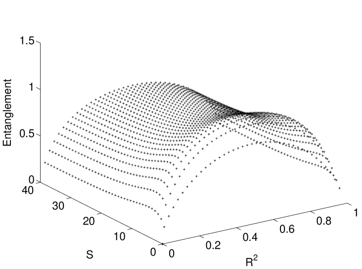
Figure 1: Entanglement of the state $|z,0\rangle$ after being passed through a beam splitter, against $S$ and $|R|^{2}$ for $|z|=3$. The maximum entanglement is given when $|R|^{2}=1/2$, for all $S$.

We now wish to see exactly how the entanglement reaches this zero limit. More precisely, we would like to determine if entanglement falls off quickly with increasing spin, such that any reasonably large spin system effectively returns a product state or if, for instance, the drop-off is monotonic. The action of a beam splitter on an input state, comprised of a spin-coherent state in one mode/arm and the vacuum state in the other, gives

$$U_{bs}|z,0\rangle=\frac{1}{(1+|z|^{2})^{S}} \sum_{n=0}^{2S}\sum_{p=0}^{n}\left\{{2S\choose n}^{1/2}{n\choose p}^{1/2}\right.$$ (9)

$$\left.\times T^{p}R^{(n-p)}\bar{z}^{n}|p,n-p\rangle\right\}.$$

We use the von Neumann entropy VonNeumann as our measure for entanglement, defined for a bipartite state $\rho_{AB}$ as

$$E=-Tr{(\rho_{A}\ln\rho_{A})}=-\sum_{i=0}^{i=2S}r_{i}\ln r_{i},$$ (10)

where $\rho_{A}=Tr_{B}(\rho_{AB})$ is the reduced density matrix of system $A$, and $r_{i}$ are its eigenvalues (and the squared Schmidt coefficients of a pure state). In our case, from Eq. (9),

$$\rho_{A} = \frac{2S!}{(1+|z|^{2})^{2S}}\sum_{p,p^{\prime}=0}^{2S}\sum_{m=0}^{\min(2S-p,2S-p^{\prime})}$$ (11)

$$\left\{\left(\frac{1}{p!p^{\prime}!(2S-m-p)!(2S-m-p^{\prime})!}\right)^{1/2}\right.$$

$$\left.\times\frac{|z|^{2m}}{m!}|T|^{2m}R^{p}\bar{R}^{p^{\prime}}\bar{z}^{p}z^{p^{\prime}}|p\rangle\langle p^{\prime}|\right\}.$$

We notice that in forming the reduced density matrix the complex phases of $R$ and $z$ are effective only up to a unitary change of basis, which does not effect its eigenvalues, and hence does not affect the entanglement. Also, $\rho_{A}$ depends on only the modulus of $T$. Thus from here on we are concerned only with the modulus of these values: $|z|$; $|R|$ and $|T|$. In Fig. 1 we plot the entanglement against $S$ and $|R|^{2}$ for $|z|=3$. For all $S$ we see a maximum entanglement for $|R|^{2}=1/2$. In fact, we found this for all $|z|$ checked between $0$ and $50$. In addition, we can prove that setting $|R|=|T|=1/\sqrt{2}$ gives the minimum linear entropy (see Appendix B), which is an upper bound to the von Neumann entropy of entanglement, and can itself be regarded as a measure of entanglement (see, for example, Bose00 ). Since it is analytically proven for the linear entropy, and it is confirmed by all our numerical evidence, and the von Neumann and linear entropy follow the same patterns in all our numerics, it is reasonable to suppose that $|R|=|T|=\sqrt{1/2}$ does indeed give maximum von Neumann entanglement. Hence from here on we take this to be the appropriate value.

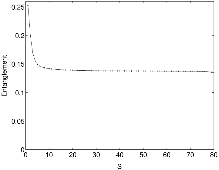
Figure 2: Entanglement of the state $|z,0\rangle$ after being passed through a beam splitter, against $S$ for $|z|=1$. As we can see, the entanglement reduces quickly at first but then more slowly. Indeed, it does not appear straight away to limit to zero (al*though we know it does).

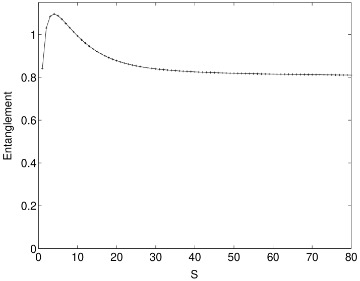
Figure 3: Entanglement of the state $|z,0\rangle$ after being passed through a beam splitter, against $S$ for $|z|=3$. Here the entanglement rises first and then tails off after around $S=40$.

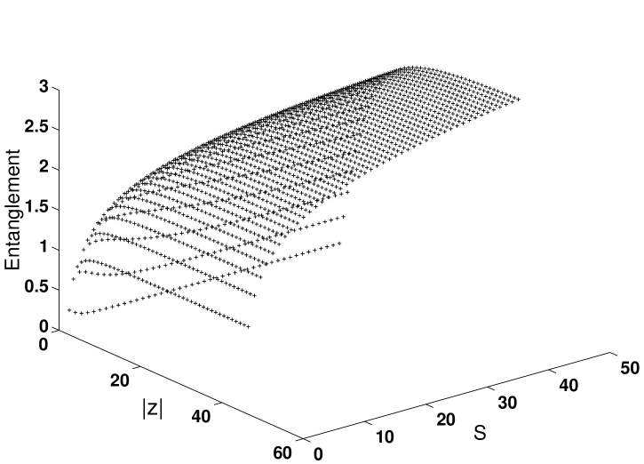
Figure 4: Entanglement of the state $|z,0\rangle$ after being passed through a beam splitter, against $S$ and $|z|^{2}$. We see the pattern of a rapid initial peak followed by very slow decrease thereafter for all $|z|$, and that an increase in $|z|$ increases the entanglement for any $S$.

Two interesting features appear. The first is that the entanglement does not quickly go to zero with increasing $S$, in fact, after an initial quick change with amplitude $|z|$, the entanglement settles to a very slow decline. The point where it settles to the slow decline is very dependent on $|z|$. For higher $|z|$ this point is both at a higher entanglement and for a higher value of $S$. For each value of $|z|$ we see first a quick and then a very slow fall from the maximum entanglement with $S$. For $|z|\leq 1$ the maximum is at the origin, for higher $|z|$ we see a peak, then the slow descent. For example, in Fig. 2 we see that the entanglement falls quickly to about $E=0.15$ at around $S=15$, and then decreases very slowly thereafter (note that, although it may not appear to, the entanglement does drop with increasing $S$ - each consecutive point after $S=15$ is lower than the previous one; the decline is just very slow). In contrast, in Fig. 3 for $|z|=3$, we see a slow tailing off from around $S=40$ at around $E=0.8$. In Fig. 4 we plot the entanglement against $S$, from $S=1/2\rightarrow 50$ for $|z|=0\rightarrow 50$. We can see that the peak where it reaches maximum is higher for higher $|z|$. In this range of $S$, the peak is not reached for $|z|$ larger than around $7$, indicating that for such $|z|$ the drop to zero is even slower and longer. Also, for any one $S$, the entanglement is higher for larger $|z|$. It looks as if the entanglement settles down to a value, dependent on $|z|$, from which it falls very slowly with increasing $S$. If the rate of decline continues as in our results, as we might expect, it would require huge $S$ to see the zero limit approached. It seems the dependency on $|z|$ is far greater than $S$.

The second feature of interest is that, for values of $|z|$ larger than unity, the entanglement initially increases with increasing $S$ (Figs. 3 and 4) and we see a peak. Since we know that the entanglement must come arbitrarily close to zero in the approach to the limit, we know it must go down from the beginning value at $S=1/2$, and we might have expected this to be a smooth fall.

The initial peak in generated entanglement, for $|z|$ larger than around $1$, is best explained by looking at the output, superposition state 9. Roughly speaking, as we increase $S$, the addition of entangled states to the superposition causes a growth in entanglement. This is then countered as more states are added, having the effect of diluting the superposition, so that the entanglement goes down for greater $S$. We do not see this for $|z|$ less than around $1$, because the coefficients for the higher entangled states in the superposition decrease for higher orders. We note that a similar phenomenon was seen in Arnesen01 , where Arnesen et al. studied the entanglement between two spin $1/2$ particles in a mixed thermal state with an external magnetic field, according to the antiferromagnetic Heisenberg model. For some field strengths, as the temperature of the chain increased, there was an initial increase in entanglement, although in the large limit the entanglement went down to zero, as we would expect for such a mixed system. The increase can be put down to the inclusion of highly entangled states in the mixture, which then becomes countered as the mixture dilutes as it extends to more states. There is also a difference here in that in our case the increase came from the addition of states to a pure superposition and in theirs they are added to the mixture.

In addition to the subject of classicality discussed in the next section, these results may be interesting for other reasons. Coherent states are useful objects, with simple and continuous parametrisation, they have many theoretical applications and allow many simplifications (see Klauder for many examples). They can be created, for example, by a rotation of the ground state of $N$ atoms Hepp73 or, in terms of the Schwinger spin states, by optical fields passing through a beam splitter (e.g., Buzek89 ). The latter can be squeezed and used to improve interferometry Kitagawa93 . Beam splitters are also useful; they are among the simplest devices implementable by experiment and have many applications, including entanglement generation itself (for example, Tan91 ); so it is valuable to understand them better in any scenario, especially one involving entanglement generation, like this one. From this point of view it might be interesting to note, for instance, that for an input state with spin $S$, there exists an optimal amplitude $|z|$ that returns the greatest entanglement.

It is also informative to consider the physical notion of a beam splitter in the sense described above. In the case of an optical state, when we use the term “beam” we usually mean literally a beam, or mode of light, that is defined by the path it takes. The action of the beam splitter is then to split the incoming photons of one mode (or path) into two, so the photons leave in a superposition of both paths. This can be written in terms of creation and annihilation operators, whence the beam splitter annihilates photons from the input path and creates photons in both output paths. With spin-coherent states this is not so clear. The analogous operators to the annihilation and creation operators are the step up and down operators. The analogy of creating a photon in a beam would be to add a unit of spin to the system (although the analogy is not exact because of different commutation relations, which change the beam splitter transformation, but broadly speaking it still accomplishes the same). With this in mind one possible interpretation of a spin $S$ system is as a symmetric superposition of $2S$ spin $1/2$ systems. Hence one can think of a beam of spin $1/2$ particles being split into two paths, where the increase of one unit of spin is equivalent to the addition of a spin $1/2$ particle. In this way, the addition of more particles increases the total spin and so makes the system more “classical”, as is the case for optical states, where the more photons there are (the higher the amplitude) the more classical the system can be said to be in terms of distinguishability and entanglement (the states out of a beam splitter are only the same as the input in the infinite limit of $\alpha$). This view of a spin $S$ system has a natural link to the Majorana representation to be discussed later, since it can be seen as an illustration of these particles.

III Comments on Classicality

We now consider what the results of the previous section could mean in terms of classicality. For the spin-coherent state, we do not see the classical feature of the Glauber state of zero entanglement generation when passed through one arm of a beam splitter, except for those with the highest spin. Indeed, the validity of the infinite limit case depends on the physical situation at hand. It is possible though to imagine when such a limit may be reasonable, for example, for a group of $10^{5}$ atoms in a Bose-Einstein condensate. For the range we explored, $S=1/2\rightarrow 50$, the entanglement is high and very dependent on $|z|$. It is to be expected that this carries on for larger $S$ too. The infinite $S$ limit offers the set of “most” classical spin-coherent states, since they are equivalent to the Glauber states and hence generate no entanglement. On this ground alone though, the spin-coherent states are no more classical than infinitely many other possible sets of states.

Then, the fact that we get an increase in entanglement as we increase $S$ is surprising, in that it indicates a reduction in classicality in this sense. Given this, we may ask if we can think of a state that is more classical in this way; for example, one that generates less entanglement and for which the entanglement decreases more rapidly with the dimension of the Hilbert space. This is a complicated problem since the only finite dimensional state to give nonentangled states through a beam splitter is the ground or vacuum state. The spin-coherent states can be arbitrarily close to this zero entanglement, but that is simply because they are arbitrarily close to the ground state in some sense. We then ask how valid this measure of classicality is. For example, we could think of other unitary transformations that would create more entanglement with the input states here; indeed, the amount of entanglement generated for a given transformation is dependent on the input state. We can talk of the entangling capacity of a unitary transformation Leifer02 , which is a maximum taken over all input states; however, to define a class of minimum entangling states for one unitary transformation does not mean it is the class of minimum entangling states for a different unitary transformation. The beam splitter transformation is a very specific example, which is important in showing one classical feature of the Glauber states, but one must ask if there is a valid reason to take this one over other transformations as a general measure. As such, we may claim that this is not an ideal measure; indeed, as a concept, the resistance to entanglement generation of a state is not well defined.

We can also consider the transition $S=1/2\rightarrow\infty$ from other points of view. A paper by Lieb in 1973 showed that in respect to the free energies of states, the spin states converge to the classical case in the thermodynamic limit of a large number and large $S$ spin states Lieb73 . This limit is very similar to the one we take; however, here Lieb talks about a thermal states, i.e., mixtures of spin-coherent states, whereas we talk only about pure states. Other discussions of classicality focus on the picture of the phase space, and how this can be said to become that of a classical state (e.g., Hall02 ). Indeed, the use of coherent states to construct and compare phase spaces can be used in many different situations, including the limit of Lieb, as was discussed in detail by Yaffe in 1982 Yaffe82 .

We can look at the natural curvature of the phase space of the set of spin-coherent states arrising from the Fubini-Study metric Provost80 . The Riemannian curvature $K$, given by $K=1/2S$ is dependent on the size of the spin system. This can be seen by imagining the phase gained by following a closed loop on the surface of the sphere Vedral02 . In general, as a vector follows a closed loop on a given space (maintaining parallel transport), it gains a phase. This phase depends on the curvature of the space; for a flat space no phase is acquired. As a spin-coherent state follows a closed loop on the sphere, it will gain a phase $\gamma=\oint\langle\psi(s)|d/ds|\psi(s)\rangle ds$, which is equal to the curvature (up to a constant), and we get $K=1/2S$. We see that for the “least” classical, $S=1/2$, state the curvature is maximum at $K=1$. This reduces smoothly and monotonically with increasing $S$ until in the infinite limit, for the “most” classical state, the curvature is zero and that of the Glauber states. This is also related to the distinguishability of states, since the distance between two states (used in the definition of this metric) increases as the size of the sphere increases. Any two points on the phase space become further apart (i.e., their overlap decreases). In this sense, the distinguishability increases. Since in classical physics objects should be distinguishable, in principle at least, this indicates an increase in classicality. We note, though, that distinguishability alone is not enough to claim classicality, for example the Fock states, which exhibit clearly nonclassical features, are orthogonal. However, it is an important feature of classical physics and one that should be mentioned in any discussion on classicality.

We now look at the change in distinguishability through the transition $S=1/2\rightarrow\infty$ for two spin-coherent states, via the Helstrom optimal measurement Helstrom . We illustrate this change using the Majorana representation Majorana32 .

One of the fundamental principles of quantum mechanics is the uncertainty relation between incompatible observables which, in turn, prohibits us from distinguishing two nonorthogonal states perfectly with one measurement. This strongly contrasts with the classical world where again, at least in principle, all states can be distinguished perfectly. We can, however, optimise our measurement strategy in quantum mechanics to give us the most reliable answer possible. One such strategy is that given by Helstrom Helstrom (see also Fuchsthesis for a very readable account) where a measurement is made to give two outcomes, one corresponding to each of the states, with a minimal probability of error. We briefly state some of those results before applying them to analysing spin-coherent states.

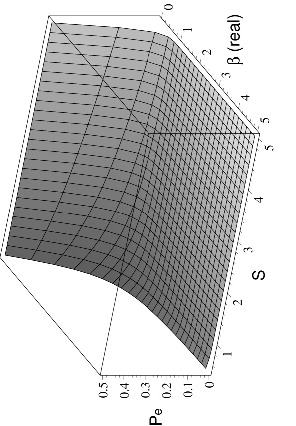
Figure 5: Probability of error of distinguishing two spin-coherent states $|0\rangle$ and $|\beta\rangle$ with a priori probabilities $p_{A}$ and $p_{B}=1-p_{A}$, respectively, against $S$ and $\beta(real)$ for $p_{A}=0.5$. The likelihood of error quickly decreases with increasing $S$ for all $\beta$.

Suppose that we are given a system we know to be in one of two states, $\rho_{A}$ or $\rho_{B}$, with probabilities $p_{A}$ and $p_{B}$, respectively. When trying to ascertain which of the two nonorthogonal states we have, we construct a two-outcome generalised measurement, or positive operator-valued measure (POVM), made up of $\hat{E}_{A}$ and $\hat{E}_{B}=\hat{\mathrm{I}\!\!1}-\hat{E}_{A}$, and associate the states with the corresponding results. The probability of being incorrect in our association, $P_{e}$, is given by

$$P_{e}=p_{A}\hbox{tr}(\hat{E}_{B}\rho_{A})+p_{B}\hbox{tr}(\hat{E}_{A}\rho_{B}).$$ (12)

For us it is important that in the case of pure states $|A\rangle$ and $|B\rangle$ this POVM becomes a projection measurement with the probability of error given by

$$P_{e} = p_{A}\hbox{tr}(\hat{E}_{B}|A\rangle\langle A|)+p_{B}\hbox{tr}(\hat{E}_{A}|B\rangle\langle B|).$$ (13)

Optimisation of this expression comes through our choice in the projection measurements. Heuristically, we wish to choose the projection spaces of $\hat{E}_{A}$ and $\hat{E}_{B}$ such that $|A\rangle$ and $\hat{E}_{B}$ are as close to orthogonal as possible; similarly for $|B\rangle$. This must be balanced against the a priori probabilities to give the minimum probability of error. When attempting to distinguish two spin-coherent states $|\alpha\rangle$ and $|\beta\rangle$ we get

$$P_{e}=\frac{1}{2}\left(1-\sqrt{1-4p_{A}p_{B}\left|\frac{(1+\alpha\bar{\beta})^{2S}}{(1+|\alpha|^{2})^{S}(1+|\beta|^{2})^{S}}\right|^{2}}\right).$$

As mentioned earlier, as $S\rightarrow\infty$, all spin coherent states become “orthogonal”, that is, the overlap tends to zero. This can be easily seen. Two spin-coherent states $|\alpha\rangle$ and $|\beta\rangle$ have overlap $|\langle\alpha|\beta\rangle|=|(1+\alpha\bar{\beta})^{2S}|/|(1+|\alpha|^{2})^{S}(1+|\beta|^{2})^{S}|$. Since $|(1+\alpha\beta^{*})^{2}|\leq|(1+|\alpha|^{2})(1+|\beta|^{2})|$, the limit in $S$ gives $\lim_{S\rightarrow\infty}|\langle\alpha|\beta\rangle|=0$ except when the equality is reached, i.e., $\alpha$ equals $\beta$, which, for all $S$, gives $|\langle\alpha|\alpha\rangle|=1$. Thus, in the limit of large $S$ all spin-coherent states become distinguishable and $P_{e}$ becomes zero, (see Fig. 5).

One very illuminating way to see the difference in the measurement process as we change $S$ or $p_{A}$/$p_{B}$ is to represent the states and the POVMs on the Riemann sphere using the Majorana representation Majorana32 - which was also used by Zimba and Penrose to recast the Kochen-Specker paradox Zimba93 . In this system, a state with spin $S$ is represented by $2S$ points on a Riemann sphere. The position of these points is given by the zeros of a complex function, constructed from the overlap of the state with a non-normalised spin-coherent state. The overlap between a non-normalised spin-coherent state $|\tilde{z}\rangle$ and $|n\rangle$, is given by

$$\langle\tilde{z}|n\rangle={2S\choose n}^{1/2}z^{n}.$$ (15)

The general state $|\psi\rangle=\sum_{n=0}^{2S}a_{n}|n\rangle$ is described (up to a global phase) by the overlap function in $z$ (also known as the “amplitude function” Arecchi72 or the “coherent-state decomposition” Leboeuf91 )

$$\psi(z)=\langle\tilde{z}|\psi\rangle = \sum_{n=0}^{2s}{2s\choose n}a_{n}z^{n},$$ (16)

$$= N\Pi_{i=1}^{2s}(z-z_{i}).$$ (17)

where $N$ is simply a normalisation constant.

The zeros of this function describe the state $|\psi\rangle$ entirely, again up to a global phase. To plot these points onto the sphere, we view them as stereographic projections from the north pole onto the complex plane going through the equator. Thus a zero on the plane marks the south pole and as the modulus of the root tends to infinity we get a point at the north pole - this happens when $\psi(z)$ is of order less than the dimension $d$ minus $1$. The multiplicity of points at the north pole is equal to the difference between the order of $\psi(z)$ and $d-1$; thus the state $|0\rangle$ is represented by $2S$ points at the north pole. The projection of $z=e^{i(\pi-\phi)}/\tan{(\theta/2)}$ onto the sphere represents the rotation of a point at the north pole through angle $\theta$ around the axis $\hat{n}=(\sin(\phi),-\cos(\phi),0)$, i.e., a point with azimuthal and polar angles $\theta$ and $\phi$, respectively. This can also be thought of as representing the rotation $\hat{R}_{\theta,\phi}$ on state $|0\rangle$.

In the $S=1/2$ case we find the well known Bloch sphere. Then, the state $|\psi\rangle=\cos{(\theta/2)}|0\rangle+e^{i\phi}\sin{(\theta/2)}|1\rangle$ has an overlap function $\psi(z)=\cos{(\theta/2)}+e^{i\phi}\sin{(\theta/2)}$ with one zero at $z=e^{i(\pi-\phi)}\tan{(\theta/2)}$, where $\theta$ and $\phi$ are the polar and azimuthal angles, respectively. We also note that the Majorana picture could equally represent a multiparticle state of $2S$ spin $1/2$ particles in a symmetric superposition. Each point represents one spin $1/2$ particle PenroseRindler . Going back to the notion of a beam of spin $S=1/2$ particles mentioned in the previous section, each point would then represent a particle in our beam.

We can make a number of observations from this definition. First, spin-coherent states are represented by $2S$ points all at the same position on the unit two-sphere. This is clear since for a spin-coherent state $|\alpha\rangle$ the overlap function is $\langle\tilde{z}|\alpha\rangle=(1+z\bar{\alpha})^{2S}/(1+|\alpha|^{2})^{S}$, which has $2S$ zeros at $-1/\bar{\alpha}$. Thus, the Majorana plot of a spin-coherent state can be seen as a representation of the rotation $\hat{R}_{\theta,\phi}$ that defines the state 5. Second, any rotation of a state $|\psi\rangle$ rotates the sphere, since when forming the overlap function [Eq. (16)], we can equally consider the rotation on $\psi$ as a reverse rotation on each of the $|\tilde{z}\rangle$’s, corresponding to the zeros, which is also a rotation of the points around the sphere. Note, though, that such a rotation can still add a phase that will not be seen on the Majorana sphere. This provides the basis for the next two points.

The modulus of the overlap between any two spin-coherent states is given entirely by the angle between their points on the sphere. This is true since any two pairs of spin-coherent states, with the same angle between them on the Majorana sphere, are only a unitary rotation apart (up to a phase); since this preserves the overlap up to a phase, any such pairs have equal overlap modulus. Any state with one or more points antipodal to a coherent state is orthogonal to that state. To see this it is sufficient to show it for the case $|\alpha\rangle=|0\rangle$, since we can simply rotate the sphere and maintain any overlap up to a phase. The set of states orthogonal to $|0\rangle$ are given by $|\alpha^{\perp}\rangle=\sum_{n=1}^{2S}a_{n}|n\rangle$. The coherent state decomposition thus has $z=0$ as one of its zeros at least; indeed, this can occur only if the state has no components in $|0\rangle$. This gives a Majorana point at the south pole, i.e., antipodal.

With this, we can begin to look at how the Helstrom discrimination strategy for two spin-coherent states can be seen in this representation. The states themselves are shown as two points on the sphere. To represent the projections we show the two resultant states after the measurement takes place, $|e_{A}\rangle$, $|e_{B}\rangle$, corresponding to $\hat{E}_{A}$ and $\hat{E}_{B}$, respectively. We can do this because the two states to be distinguished will both collapse onto the same one of two resultant states. This is because any projection we make will be on the two-dimensional subspace of the two states, since to project outside this space would not be optimal. Hence, they project onto the same pair of states in this subspace.

The first thing we notice is that for any $S$ these states give Majorana points that lie on a circle on the surface of the sphere. This is, in fact, the case for any state that is a superposition of two spin-coherent states. For any complex coefficients $a$ and $b$, the state $|\psi\rangle=a|0\rangle+b|\beta\rangle$ gives overlap function zeros that lie on a circle of radius $r=\left|a/b\right|^{1/2S}(1+|\beta|^{2})^{1/2}/|\beta|$, centred at $-1/\bar{\beta}$ on the complex plane. The stereographic projection preserves circles and angles Eves ; hence the Majorana points lie on a circle also (since this is true for the above superposition, it is true for any superposition of two coherent states because we can always rotate the pair so that one state is $|0\rangle$ and maintain the geometry). Furthermore, the radius and position of these circles relate back to the overlap of the states and their a priori probabilities, although the relationships are complicated, and we will talk about trends qualitatively only.

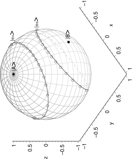
Figure 6: Majorana projection of two coherent states $|A\rangle$ and $|B\rangle$, and the states postprojection $|e_{A}\rangle$ and $|e_{B}\rangle$, for $S=10$ and $p_{A}=p_{B}=0.5$.

In Fig. 6 we see the Majorana projection of two spin-coherent states, given by two black points, and the states post projection, given by the grey points, which exist on two circles, for $S=10$. State $|A\rangle=|0\rangle$ is on the north pole and state $|B\rangle=|-i\rangle$ is at $(1,0,0)$. The a priori probabilities are set at $p_{A}=p_{B}=0.5$.

We can now look at how when changing the a priori probabilities $p_{A}$/$p_{B}$ and $S$, the Helstrom measurements we make, found from the minimisation of Eq. (13), also change. For any fixed spin, as the a priori probability of $|A\rangle$ increases, the circle of the corresponding projection $\hat{E}_{A}$ closes in around the state, until it becomes that state. That is, $|e_{A}\rangle\rightarrow|A\rangle$, as we would expect for minimisation of the error (13). The other circle, for projection $\hat{E}_{B}$, widens until it becomes the state orthogonal to $|A\rangle$ in the $|A\rangle$,$|B\rangle$ subspace ($|A_{\perp}\rangle$), this gives the circle whose width allows one point to exist antipodal to the Majorana point of $|A\rangle$. The opposite to this occurs should $p_{B}$ increase.

Keeping $p_{A},p_{B}$ fixed and increasing $S$, both circles become larger, as $|e_{A}\rangle\rightarrow|B_{\perp}\rangle$ and $|e_{B}\rangle\rightarrow|A_{\perp}\rangle$. This shows the reason for the decrease in probability of error with $S$. As $S$ increases, the states $|A\rangle$ and $|B\rangle$ become more orthogonal; this allows the projection POVMs to change to become more orthogonal to the anticorresponding states, in accordance with the minimisation of Eq. (13), seen by the growth of the circles, where $P_{e}$ then reduces with increasing $S$. Therefore, the smooth growth of the projection circles illustrates that, within this distinguishability criterion for classicality, spin-coherent states approach the “classical”, Glauber, states with the increase of spin. This is in contrast with the previous criterion based on entanglement generation where we see a brief increase of entanglement with spin.

IV Conclusion

In this paper, we have examined the transition of spin-coherent states from spin $S=1/2$ to the limit $S\rightarrow\infty$ with respect to the generation of entanglement through a beam splitter. We gave an alternative proof that, as the spin tends to infinity, the spin-coherent states tend to the infinite amplitude limit of the Glauber states. From this proof we can easily see that this is not unique to spin coherent states; indeed, there are infinitely many sets of states for which this is true. The spin-coherent state does represent an element of these that achieves minimum uncertainty.

We have studied the entanglement generation of spin-coherent states for the specific case where they are sent through one arm of a 50:50 beam splitter and a vacuum through the other. Two main features were observed. The first is that the entanglement of the output states depends heavily on $|z|$, more than $S$. For all $|z|$, after an initial quick change with $S$, the entanglement settles to a very slow, almost flat decline. The entanglement at which this slow tailing off begins is very dependent on $|z|$ and is higher for larger $|z|$. To see the high $S$ near zero entanglement, one would need a system of huge spin number. The relevance of this limit is very dependent on the physical system. In our numerics we considered only up to spin $S=50$, but we may see a significantly low resultant entanglement for systems with extremely large $S$, for example, of the order of $10^{5}$ spin $1/2$ atoms. The second interesting feature is that for $|z|>1$ the entanglement initially rose with $S$.

We then discussed this transition in terms of classicality. The high dependence on $|z|$, very slow decline to zero, and increase of entanglement (thus dip in this sense of classicality) are indicators that this measure may be inadequate as a universal signature of classicality, as we found. The value in these results is in the understanding of a beam splitter as an entanglement generator, with respect to which it is also found that the generated entanglement increases with amplitude $z$, and that for any spin $S$ we can find an amplitude with $|z|$ that gives the maximum entanglement at output. In a sense we have sacrificed the generality of this result as a classicality measure for its simplicity and applicability.

We listed briefly some examples of other ways the transition can be looked at in terms of classicality. The large $S$ limit discussed by Lieb also leads to a classical description, in terms of free energies. The change in phase space as we change $S$ also indicates a transition to classicality in some sense. We then focused on distinguishability in terms of state discrimination using the Helstrom optimal measurement strategy and illustrated it using the Majorana picture. The geometry of the states and the Helstrom POVMs is simple, and allows us to illustrate easily the changes affecting the probability of error for the measurement. A spin-coherent state is simply one point on the sphere and the POVMs are represented by circles of points. The decrease in probability of error with an increase in $S$ is seen by the increase in the diameter of the circles on the sphere representing the measurements. We reiterate that distinguishability does not constitute classicality in its own right. The standard example of Fock states makes is an example. Indeed none of these measures give a common result; they all follow different declines and cannot be said to be equivalent exactly in the transition regime. Distinguishability is important and although not a complete description, if we want to look at classicality, we must discuss this, as we must all areas.

Possible extensions of this work would naturally include the move to considering the mixed case as in Kim02 and Xiang-bin02 . A consideration of a thermal mixture of states, as in Lieb’s calculation, may offer interesting results in terms of entanglement. It would also be interesting for future work to create common criteria for “classicality measures” or indicators of (pure) states. It seems that one common feature that should be imposed is the increase in classicality with the size of a system, or the number of subsystems involved, so that it appears classical in the large macroscopic limit. An important problem, brought to light in the discussion of the beam splitter, is the assignment of classicality in terms of entanglement. A classical system should be inefficient at generating entanglement within itself, but on the other hand, should be able to strongly entangle with its environment (this is required, for example, in decoherence models). It is not at all clear that there exists a single measure that would capture all these desirable properties and this remains a challenging open problem.

Acknowledgements. We would like to thank William Irvine, Manfred Lein, and Stefan Scheel for very useful discussions on the subject of this paper and Jens Eisert for critical reading of the proofs involved. This work was sponsored by the Engineering and Physical Sciences Research Council, the European Community, the Elsag spa and the Hewlett-Packard company.

Appendix A

Glauber states are defined as Glauber63

$$|\alpha\rangle = \exp\left(\alpha\hat{a}^{{\dagger}}-\frac{1}{2}|\alpha|^{2}\right)|0\rangle$$ (18)

$$= \exp\left(-\frac{1}{2}|\alpha|^{2}\right)\sum_{n=0}^{\infty}\frac{\alpha^{n}}{(n!)^{1/2}}|n\rangle.$$

We wish to show that, by appropriate substitution, the spin-coherent state (6) is equal to a subclass of Glauber states as $S$ tends to infinity. We know that for any two different spin-coherent states, the overlap tends to zero as $S$ tends to infinity; thus the “amplitude” $\alpha$ for the optical case must tend to infinity as $S$ does. We set $\alpha=\sqrt{2S}\bar{z}$. Substituting this into Eq. (6) we get

$$|z^{\prime}\rangle = \frac{1}{(1+\frac{|\alpha|^{2}}{2S})^{S}}\ \sum_{n=0}^{2S}{2S\choose n}^{1/2}\left(\frac{\alpha}{2S}\right)^{n}|n\rangle.$$ (19)

To prove the equivalence of the two states in the infinite limit, it is sufficient to show that the overlap of a Glauber state $|\alpha\rangle$ and such a spin-coherent state goes to $1$ (i.e., they are the same state). Thus, we wish to prove that

$$\lim_{S\rightarrow\infty}\langle\alpha|z^{\prime}\rangle = \lim_{S\rightarrow\infty}\left\{\exp{\left(-\frac{1}{2}|\alpha|^{2}\right)}\frac{1}{(1+\frac{|\alpha|^{2}}{2S})^{S}}\right.$$ (20)

$$\left.\times\sum_{n=0}^{2S}\left(\frac{2S!}{(2S-n)!(2S)^{n}}\right)^{1/2}\frac{|\alpha|^{2n}}{n!}\right\}$$

$$= 1.$$

Let us first look at the summation.
Lemma. For all $A\in\mathbb{R}^{+}$,

$$\lim_{n\rightarrow\infty}\sum_{p=0}^{n}\left(\frac{n!}{(n-p)!n^{p}}\right)^{1/2}\frac{A^{p}}{p!}=\sum_{p=0}^{\infty}\frac{A^{p}}{p!}.$$ (21)

Proof. We will use the method of showing that the upper and lower bounds to $\langle\alpha|z^{\prime}\rangle$ coincide as $S$ tends to infinity. Since each term in the sum is positive, one upper bound of the left hand side of Eg. (21) can be found by taking the sum to infinity. Thus

$$\lim_{n\rightarrow\infty}\sum_{p=0}^{n}\left(\frac{n!}{(n-p)!n^{p}}\right)^{1/2}\frac{A^{p}}{p!} \leq \lim_{n\rightarrow\infty}\sum_{p=0}^{\infty}\left(\frac{n!}{(n-p)!n^{p}}\right)^{1/2}\frac{A^{p}}{p!}$$

$$\leq \sum_{p=0}^{\infty}\frac{A^{p}}{p!},$$

where the last line is given by taking the limit inside the sum, which we are allowed to do since each term converges.

We then find a lower bound by taking the sum to some finite $m$, so

$$\lim_{n\rightarrow\infty}\sum_{p=0}^{n}\left(\frac{n!}{(n-p)!n^{p}}\right)^{1/2}\frac{A^{p}}{p!} \geq \lim_{n\rightarrow\infty}\sum_{p=0}^{m}\left(\frac{n!}{(n-p)!n^{p}}\right)^{1/2}\frac{A^{p}}{p!}.$$

However, taking the infinite limit of $m$ this inequality still holds, since it is true for any finite $m$ and so it is true for any arbitrarily small distance from the limit, so the limit can at most be equal. This gives the same upper as lower bound; hence

$$\lim_{n\rightarrow\infty}\sum_{p=0}^{n}\left(\frac{n!}{(n-p)!n^{p}}\right)^{1/2}\frac{A^{p}}{p!} = \lim_{n\rightarrow\infty}\sum_{p=0}^{\infty}\left(\frac{n!}{(n-p)!n^{p}}\right)^{1/2}\frac{A^{p}}{p!}$$ (24)

$$= \sum_{p=0}^{\infty}\frac{A^{p}}{p!}$$

$$= \exp(A).$$

Since the normalisation and the summation in Eq. (20) converge with increasing $n$, the limit of the product is the product of the limits and thus

$$\lim_{S\rightarrow\infty}\langle\alpha|z^{\prime}\rangle = \exp{\left(-|\alpha|^{2}\right)}\exp{\left(|\alpha|^{2}\right)}$$ (25)

$$= 1.$$

Interestingly, this is also true of any state $|\psi\rangle=\sum_{n=0}^{d-1}f(n,d)[A^{n}/(n!)^{1/2}]|n\rangle$ such that $f(n,d)>0,\forall n,d\in\mathbb{N}$, and $f(n,d)$ converges to $1$ in $n$, for all $p$, for example, $|z\rangle=\exp\left(-\frac{1}{2}|z|^{2}\right)\sum_{p=0}^{n}(z^{p}/p!)|p\rangle$. There are infinitely many such functions and therefore there are infinitely many states that will tend to the Glauber state in the limit, as stated in Sec. II.

Appendix B

Linear entropy is an upper bound to the von Neumann entropy and is defined as

$$S_{lin}=1-Tr\left(\rho_{A}^{2}\right).$$ (26)

The linear entropy of the two output “beams” is given by

$$S_{lin} = 1-\frac{(2S!)^{2}}{(1+|z|^{2})^{4S}}\sum_{p,p^{\prime}=0}^{2S}\sum_{m,m^{\prime}}^{min(2S-p,2S-p^{\prime})}\left(\frac{|z|^{m+m^{\prime}+p+p^{\prime}}}{m!m^{\prime}!}\right.$$ (27)

$$\left.\times\frac{1}{\sqrt{(2S-m-p)!(2S-m-p^{\prime})!}}\right.$$

$$\left.\times\frac{1}{\sqrt{(2S-m^{\prime}-p)!(2S-m^{\prime}-p^{\prime})}}\right.$$

$$\left.\times|R|^{2(p+p^{\prime})}|T|^{2(m+m^{\prime})}\right),$$

with $|R|^{2}+|T|^{2}=1$. Differentiating this with respect to $|R|$, we have

$$\frac{dS_{lin}}{d|R|} = -\sum_{p,p^{\prime}=0}^{2S}\sum_{m,m^{\prime}}^{min(2S-p,2S-p^{\prime})}\left\{f(|z|,S,m,m^{\prime},p,p^{\prime})\right.$$ (28)

$$\times \left.\left(|R|^{(p+p^{\prime}-1)}(p+p^{\prime})(1-|R|)^{(m+m^{\prime})}\right.\right.$$

$$\left.\left.-(1-|R|)^{(m+m^{\prime}-1)}(m+m^{\prime})|R|^{(p+p^{\prime})}\right)\right\},$$

where

$$f(|z|,S,m,m^{\prime},p,p^{\prime})=\frac{(2S!)^{2}}{(1+|z|^{2})^{4S}}\left(\frac{|z|^{m+m^{\prime}+p+p^{\prime}}}{m!m^{\prime}!}\right.$$

$$\left.\times\frac{1}{\sqrt{(2S-m-p)!(2S-m-p^{\prime})!}}\right.$$

$$\left.\times\frac{1}{\sqrt{(2S-m^{\prime}-p)!(2S-m^{\prime}-p^{\prime})}}\right).$$ (29)

Using the symmetry of the summations and the symmetry of $f(|z|,S,m,m^{\prime},p,p^{\prime})$, one can see that Eq. (28) gives a zero at $|R|=|T|=1/\sqrt{2}$. Hence the linear entropy is maximum, for any $S$ and $z$, when $|R|=|T|=1/\sqrt{2}$.

References

- [1] M. Gell-Mann and J. Hartle. Phys. Rev. D, 47(3345), 1993.
- [2] R. J. Glauber. Phys. Rev., 131(2766), 1963.
- [3] J. R. Klauder and B. Skagerstam. Coherent states. World Scientific, Singapore, 1985.
- [4] J. R. Klauder. 2001. Contribution to the 7th ICUSSR Conference, June 2001, quant-ph/9601020.
- [5] J. M. Radcliffe. J. Phys. A, 4(313-323), 1971.
- [6] F. T. Arecchi, E. Courtens, R. Gilmore, and H. Thomas. Phys. Rev. A, 6(2211), 1972.
- [7] Y. Aharonov, D. Falkoff, E. Lerner, and H. Pendelton. Ann. Phys., 39(498-512), 1966.
- [8] M. S. Kim, W. Son, V. Busek, and P. L. Knight. Phys. Rev. A, 65(032323), 2002.
- [9] Wang Xiang-bin. 2002. quant-ph/0204039.
- [10] W. Vogel. Phys. Rev. Lett, 84(1849), 2000.
- [11] M.C. Arnesen, S. Bose, and V. Vedral. Phys. Rev. Lett., 87(017901), 2001.
- [12] E. Majorana. Nuovo Cimento, 9(43-50), 1932.
- [13] C. W. Helstrom. Quantum Detection and Estimation Theory. Academic Press, New York, 1976.
- [14] C. A. Fuchs. Phd thesis. University of New Mexico, quant-ph/9601020.
- [15] N. Gisin. Phys. Lett. A, 242(1), 1998.
- [16] R. A. Campos, B. E. A. Saleh, and M. C. Teich. Phys. Rev. A, 40(1371), 1989.
- [17] T. Holstein and H. Primakoff. Phys. Rev., 58(1098), 1940.
- [18] J. von Neumann. Mathematical Foundations of Quantum Mechanics. (Eng. translation by R. T. Beyer), Princeton University Press, Princeton, 1955.
- [19] S. Bose and V. Vedral. Phys. Rev. A, 61(040101), 2000.
- [20] K. Hepp and E. H. Lieb. Phys. Rev. A, 8(2517), 1973.
- [21] V. Buẑek and T. Quang. J. Opt. Soc. Am. B, 6(2447), 1989.
- [22] M. Kitagawa and M. Ueda. Phys. Rev. A, 47(5138), 1993.
- [23] S. M. Tan, D. F. Walls, and M. J. Collett. Phys. Rev. Lett., 66(252), 1991.
- [24] M. S. Leifer, L. Henderson, and N. Linden. 2002. quant-ph/9601020.
- [25] E. H. Lieb. Commun. Math. Phys., 31(327), 1973.
- [26] B. C. Hall and J. Mitchell. quant-ph/0203142.
- [27] L. G. Yaffe. Rev. Mod. Phys., 54(407), 1982.
- [28] J. P. Provost and G. Vallee. Commun. Math. Phys. , 76(289-301), 1980.
- [29] V. Vedral. 2002. quant-ph/0212133.
- [30] J. Zimba and R. Penrose. Stud. Hist. Phil. Sci., 24(697-720), 1993.
- [31] P. Leboeuf. J. Phys. A: Math. Gen., 24(4575), 1991.
- [32] R. Penrose and W. Rindler. Spinors and Space Time. Vol.1: Two Spinor Calculus and Relative Fields. Cambridge University Press, Cambridge, check edition, 1984.
- [33] H. Eves. A Survey of Geometry. Allyn and Bacon, Inc. Boston, 1963.