Non-Perturbative Renormalization Group Analysis
in Quantum Mechanics

1 Introduction

The non-perturbative renormalization group (NPRG) has been formulated through analyses of critical phenomena[1] and applied to non-perturbative studies of statistical mechanics and quantum field theories. It has been established as a powerful tool for analyses of non-perturbative dynamics in systems of many (infinite) degrees of freedom, because it allows for the evaluation of fluctuations without recourse to perturbation series. Several types of non-perturbative (exact) renormalization group equations have been derived by integration with scale decomposition and have been applied to various systems.[2, 3, 4, 5, 6, 7, 8, 9] In this article, we apply the NPRG method to quantum mechanical systems, that is, systems of finitely many degrees of freedom[2, 6, 10] to analyze their non-perturbative dynamics.

Generally, there are two types of non-perturbative quantities. One corresponds to the summation of all orders of a perturbative series, which could be related to Borel resummation.[11] The other is an essential singularity with respect to a coupling constant $\lambda_{0}$, which has a structure like $e^{-\frac{1}{\lambda_{0}}}$.[12, 13] We are not able to expand such a singular contribution around $\lambda_{0}=0$. A singularity of this type appears in the case of quantum tunneling. For example, in a symmetric double well system, there are two degenerate energy levels at each minimum, which are mixed through tunneling to generate an energy gap $\mathchar 28929\relax E\sim e^{-\frac{1}{\lambda_{0}}}$. The exponential factor is known to result from the free energy of topological configurations, i.e., instantons.

In this article, we first summarize how to analyze quantum mechanical systems using the concept of NPRG and check to what extent NPRG can be used to evaluate non-perturbative effects quantitatively. The NPRG equation we employ here is a local potential approximated Wegner-Houghton (LPA W-H) equation,[14, 15] which we use to analyze quantum anharmonic oscillators and asymmetric double well systems. In contrast to the symmetric double well system, the standard instanton method does not work for an asymmetric potential, and the much more sophisticated method of the valley instanton has been developed for their treatment.[30, 31] The NPRG method is found to work for asymmetric potentials as well as for symmetric potentials, because NPRG does not rely on parity symmetry.

We proceed to analyses of more complicated systems, supersymmetric quantum mechanics (SUSY QM) and many particle systems. SUSY QM is a toy model for dynamical SUSY breaking.[33, 34] Although, in general, there is no spontaneous symmetry breaking in systems with finitely many degrees of freedom, some extraordinary symmetries, such as SUSY, can be broken even in quantum mechanics. SUSY breaking is a highly non-perturbative phenomenon because of the non-renormalization theorem, and we will see that NPRG should be applicable for non-perturbative SUSY breaking.

In addition, analyses of quantum many particle systems have become very important with recent developments in nano-technology. Solving the problem of how the quantum coherence of a variable of a target system is affected by other variables (the environment) is quite important. For example, it is necessary for realization of qubit for quantum computers. However, standard methods that are well suited for treating systems of one degree of freedom, the Schrödinger equation, instanton, etc., do not work well in such complicated systems. We believe that NPRG is versatile enough to analyze such systems. As a first step, we analyze quantum tunneling phenomena in two particle quantum systems.

2 Non-perturbative renormalization group

In this section, we briefly summarize the formulation of NPRG with $D$-dimensional real scalar field theory.

2.1 Scale decomposition

In the NPRG method, the theory is defined by the Wilsonian effective action $S_{\mathchar 28931\relax}[\phi]$. This is an effective theory with an ultraviolet energy cutoff $\mathchar 28931\relax$:

$$Z=\int{\cal D}\phi~{}e^{-S_{\mathchar 28931\relax}[\phi]}.$$ (1)

We decompose the path integration variable $\phi(p)$ into two parts with respect to the momentum scale $p$ as

$$\phi(p)=\left\{\begin{array}[]{ll}\phi_{<}(p)&~{}~{}~{}~{}~{}~{}~{}~{}~{}~{}~{}~{}\!0\leq|p|<\mathchar 28931\relax-{\mit\mathchar 28929\relax}\mathchar 28931\relax~{}~{}:{\rm lower~{}modes},\\ \phi_{s}~{}(p)&~{}~{}~{}\mathchar 28931\relax-{\mit\mathchar 28929\relax}\mathchar 28931\relax\leq|p|\leq\mathchar 28931\relax~{}~{}~{}~{}~{}~{}~{}~{}~{}~{}:~{}{\rm shell~{}modes},\end{array}\right.$$

and transform the partition function $Z$ as follows:

$$Z = \int{\cal D}\phi_{<}~{}{\cal D}\phi_{s}~{}e^{-S_{\mathchar 28931\relax}[\phi_{<}+\phi_{s}]},$$ (3)

$$= \int{\cal D}\phi_{<}~{}e^{-S_{\mathchar 28931\relax}[\phi_{<}]}\int{\cal D}\phi_{s}~{}e^{-S_{\mathchar 28931\relax}[\phi_{s}]}~{}e^{-S_{\mathchar 28931\relax}^{\rm~{}\!int}[~{}\!\phi_{<},~{}\phi_{s}~{}\!]},$$

$$= \int{\cal D}\phi_{<}~{}e^{-S_{\mathchar 28931\relax}[\phi_{<}]}\left<~{}e^{-S_{\mathchar 28931\relax}^{\rm~{}\!int}[~{}\!\phi_{<},~{}\phi_{s}~{}\!]}\right>_{\phi_{s}},$$

$$= \int{\cal D}\phi_{<}~{}e^{-S_{\mathchar 28931\relax}[\phi_{<}]}~{}e^{-{\mit\mathchar 28929\relax}S_{\mathchar 28931\relax}[\phi_{<}]},$$

$$= \int{\cal D}\phi_{<}~{}e^{-S_{\mathchar 28931\relax-{\mit\mathchar 28929\relax}\mathchar 28931\relax}[\phi_{<}]},$$

where

$${\mit\mathchar 28929\relax}S_{\mathchar 28931\relax}[\phi_{<}]\equiv-\log\left<~{}e^{-S_{\mathchar 28931\relax}^{\rm~{}\!int}[~{}\!\phi_{<},~{}\phi_{s}~{}\!]}\right>_{\phi_{s}}\equiv\int{\cal D}\phi_{s}~{}e^{-S_{\mathchar 28931\relax}[\phi_{s}]}~{}e^{-S_{\mathchar 28931\relax}^{\rm~{}\!int}[~{}\!\phi_{<},~{}\phi_{s}~{}\!]}.$$ (4)

We understand the shell mode path integral $\left<\cdot\cdot\cdot\right>_{\phi_{s}}$ as the renormalization transformation. If we evaluate it by perturbative expansion with respect to coupling constants, we obtain the so-called perturbative renormalization group equations.[16] Of course such equations are valid only in the weak coupling limit. Instead, we take the limit ${\mit\mathchar 28929\relax}\mathchar 28931\relax\to 0$ to define NPRG equation, which is the fundamental procedure.[14]

2.2 Derivation of the NPRG equation

Taking the limit ${\mit\mathchar 28929\relax}\mathchar 28931\relax\to 0$, we can express the renormalization transformation as a differential equation,

$$\frac{\partial S_{\mathchar 28931\relax}}{\partial\mathchar 28931\relax}=\lim_{{\mit\mathchar 28929\relax}\mathchar 28931\relax\to 0}\frac{S_{\mathchar 28931\relax}-S_{\mathchar 28931\relax-{\mit\mathchar 28929\relax}\mathchar 28931\relax}}{{\mit\mathchar 28929\relax}\mathchar 28931\relax}=\lim_{{\mit\mathchar 28929\relax}\mathchar 28931\relax\to 0}\frac{1}{{\mit\mathchar 28929\relax}\mathchar 28931\relax}~{}{\rm log}~{}\left<~{}e^{-S_{\mathchar 28931\relax}^{\rm~{}\!int}[~{}\!\phi_{<},~{}\phi_{s}~{}\!]}\right>_{\phi_{s}}.$$ (5)

Then, we can expand $S_{\mathchar 28931\relax}[\phi]$ as power series in $\phi_{s}$:

$$S_{\mathchar 28931\relax}\left[\phi\right] = S_{\mathchar 28931\relax}\left[\phi_{<}\right]+\int_{\rm shell}\left.{\delta S_{\mathchar 28931\relax}\over\delta\phi\left(p\right)}\right|_{\phi_{s}=0}\!\!\!\!\!\!\cdot\phi_{s}\left(p\right)$$ (6)

$$+~{}{1\over 2}\int\int_{\rm shell}\phi_{s}(p)\cdot\left.{\delta^{2}S_{\mathchar 28931\relax}\over\delta\phi(p)\delta\phi(q)}\right|_{\phi_{s}=0}\!\!\!\!\!\!\cdot\phi_{s}(q)~{}+~{}O({\mit\mathchar 28929\relax}\mathchar 28931\relax^{2}).$$

Since an $O({\mit\mathchar 28929\relax}\mathchar 28931\relax)$ calculation is required for the evaluation of the derivative (5), the shell mode path integral $\left<\cdot\cdot\cdot\right>_{\phi_{s}}$ can be evaluated exactly using a Gaussian integration. Then, the fundamental differential equation is derived as

$$\mathchar 28931\relax\frac{\partial S_{\mathchar 28931\relax}}{\partial\mathchar 28931\relax}=~{}\frac{\mathchar 28931\relax}{2}\int_{\rm shell}\left\{-~{}{\rm log}\left(\left.{\delta^{2}S_{\mathchar 28931\relax}\over\delta\phi_{p}\delta\phi_{-p}}\right|\right)+\left.{\delta S_{\mathchar 28931\relax}\over\delta\phi_{p}}\right|\left(\left.{\delta^{2}S_{\mathchar 28931\relax}\over\delta\phi_{p}\delta\phi_{-p}}\right|\right)^{-1}\!\!\!\left.{\delta S_{\mathchar 28931\relax}\over\delta\phi_{-p}}\right|~{}\right\}.$$ (7)

This is known as the Wegner-Houghton equation.[14] It represents exactly the cutoff $\mathchar 28931\relax$ dependence of the Wilsonian effective action $S_{\mathchar 28931\relax}$. Its right-hand side is generally called a $\beta$ functional.

2.3 Approximations

Although the Wegner-Houghton equation is exact, we cannot solve it without some approximation in practice. In this article we employ the local potential approximation (LPA), which means that we ignore corrections to derivative interactions. It can be considered the leading order of the derivative expansion of $S_{\mathchar 28931\relax}$,

$$S_{\mathchar 28931\relax}[\phi]=\int d^{D}x~{}\left\{~{}V_{\mathchar 28931\relax}[\phi]+\frac{1}{2}K_{\mathchar 28931\relax}[\phi]\!~{}\partial_{\mu}\phi\partial_{\mu}\phi+\cdot\cdot\cdot\right\}.$$ (8)

To make this approximation, we substitute the zero mode for the lower mode $\phi_{<}(p)$:

$$\phi_{<}(p)\to\varphi~{}(2\pi)^{D}\delta^{D}(p).$$ (9)

The local potential approximated Wegner-Houghton (LPA W-H) equation is then obtained as follows:

$$\mathchar 28931\relax{\partial V_{\mathchar 28931\relax}\over\partial\mathchar 28931\relax} = -~{}\!\frac{A_{D}}{2}~{}\!\mathchar 28931\relax^{D}~{}\!\log\left(1+\frac{1}{\mathchar 28931\relax^{2}}\frac{\partial^{2}V_{\mathchar 28931\relax}}{\partial\varphi^{2}}\right),$$ (10)

$$A_{D} \equiv \frac{\int d\mathchar 28938\relax_{D}}{(2\pi)^{D}}.$$ (11)

This is a two-dimensional partial differential equation for $V_{\mathchar 28931\relax}(\varphi).$[15] Its right-hand side is called a $\beta$ function. We solve it mainly using numerical methods.

To obtain an intuitive understanding of this equation, we proceed to further approximation, the operator expansion. We expand $V_{\rm eff}$ as power series in $\varphi$:

$$V_{\mathchar 28931\relax}\left(\varphi\right) = \sum_{n=0}^{N}\frac{a_{n}(\mathchar 28931\relax)}{n!}\varphi^{n}.$$ (12)

The partial differential equation is then reduced to a set of ordinary differential equations for the coupling constants $\{{a}_{n}(\mathchar 28931\relax)\}$:

$$\mathchar 28931\relax{d{a}_{0}\over d\mathchar 28931\relax} = -\frac{A_{D}}{2}~{}\!\mathchar 28931\relax^{D}~{}\!\log\left(\frac{\mathchar 28931\relax^{2}+{a}_{2}}{\mathchar 28931\relax^{2}}\right),$$ (13)

$$\mathchar 28931\relax{d{a}_{1}\over d\mathchar 28931\relax} = -\frac{A_{D}}{2}~{}\!\mathchar 28931\relax^{D}~{}\!\left[{a}_{3}\over\mathchar 28931\relax^{2}+{a}_{2}\right],$$ (14)

$$\mathchar 28931\relax{d{a}_{2}\over d\mathchar 28931\relax} = -\frac{A_{D}}{2}~{}\!\mathchar 28931\relax^{D}~{}\!\left[{{a}_{4}\over\mathchar 28931\relax^{2}+{a}_{2}}-{{a}_{3}^{2}\over\left(\mathchar 28931\relax^{2}+{a}_{2}\right)^{2}}\right],$$ (15)

$$\mathchar 28931\relax{d{a}_{3}\over d\mathchar 28931\relax} = -\frac{A_{D}}{2}~{}\!\mathchar 28931\relax^{D}~{}\!\left[{{a}_{5}\over\mathchar 28931\relax^{2}+{a}_{2}}-{3{a}_{4}{a}_{3}\over\left(\mathchar 28931\relax^{2}+{a}_{2}\right)^{2}}+{2{a}_{3}^{3}\over\left(\mathchar 28931\relax^{2}+{a}_{2}\right)^{3}}\right],$$ (16)

$$\mathchar 28931\relax{d{a}_{4}\over d\mathchar 28931\relax} = -\frac{A_{D}}{2}~{}\!\mathchar 28931\relax^{D}~{}\!\left[{{a}_{6}\over\mathchar 28931\relax^{2}+{a}_{2}}-{4{a}_{5}{a}_{3}\over\left(\mathchar 28931\relax^{2}+{a}_{2}\right)^{2}}-{3{a}_{4}^{2}\over\left(\mathchar 28931\relax^{2}+{a}_{2}\right)^{2}}\right.$$

$$~{}~{}~{}~{}~{}~{}~{}~{}~{}~{}~{}~{}~{}~{}~{}~{}~{}~{}~{}~{}~{}~{}~{}~{}~{}~{}~{}~{}~{}~{}~{}~{}~{}~{}~{}~{}~{}~{}~{}~{}~{}~{}~{}\left.+\frac{12{a}_{4}{a}_{3}^{2}}{\left(\mathchar 28931\relax^{2}+{a}_{2}\right)^{3}}-\frac{6{a}_{3}^{4}}{\left(\mathchar 28931\relax^{2}+{a}_{2}\right)^{4}}\right],$$

$$\vspace{3cm}\vdots~{}~{}~{}~{}~{}~{}~{}~{}~{}~{}~{}~{}~{}~{}~{}~{}~{}~{}~{}~{}~{}~{}~{}~{}~{}~{}~{}~{}~{}~{}~{}~{}~{}~{}~{}~{}~{}~{}~{}~{}~{}~{}~{}~{}~{}~{}~{}~{}~{}~{}~{}~{}~{}~{}~{}~{}~{}~{}~{}~{}~{}~{}~{}~{}~{}~{}~{}~{}~{}~{}~{}~{}~{}~{}~{}~{}~{}~{}~{}~{}.$$

If the results of these equations converge as the order of the truncation, $N$, becomes large, we regard them as solutions of the LPA W-H equation.[17] This expansion allows us to treat differential equations more easily and to understand the origin and structure of quantum corrections physically. For example, a correction to odd $n$ couplings cannot be generated from even $n$ couplings only. This implies that if we choose an initial potential $V_{0}(\varphi)$ as $Z_{2}(\varphi\leftrightarrow-\varphi)$ symmetric, the solutions of the RG equations flow in $Z_{2}$ symmetric subspace; that is, the NPRG equation does not break the global symmetry of the system. However, we should note that in some extreme cases, the operator expansion is not good, and leads to pathological behavior, as seen in §4.

The constant part of $V_{\mathchar 28931\relax}$, $a_{0}$, is given by the vacuum bubble diagrams and is usually ignored. However, we retain it here, because it plays a crucial role in supersymmetric theories.

3 NPRG analysis of quantum mechanical systems

Making use of the LPA W-H equation, we analyze systems in quantum mechanics, which is $D=1$ real scalar theory with a single dynamical variable, $x(\tau)$.[10]

3.1 Physical quantities

The LPA W-H equation for quantum mechanics is given as follows:

$$\mathchar 28931\relax\frac{\partial V_{\mathchar 28931\relax}}{\partial\mathchar 28931\relax} = -~{}\!\frac{1}{2\pi}~{}\!\mathchar 28931\relax~{}\!\log\left(1+\frac{1}{\mathchar 28931\relax^{2}}\frac{\partial^{2}V_{\mathchar 28931\relax}}{\partial x^{2}}\right).$$ (18)

We solve it by lowering $\mathchar 28931\relax$ from the initial cutoff $\mathchar 28931\relax_{0}$, where the initial potential $V_{\mathchar 28931\relax_{0}}$ is given by the potential term $V_{0}(x)$ in the original action,

$$S[x]=\int d\tau~{}\left\{~{}\frac{1}{2}\!~{}\dot{x}^{2}+V_{0}(x)\right\}.$$ (19)

In the infrared limit $\mathchar 28931\relax\to 0$, we obtain the effective potential $V_{\rm eff}(x)=\lim_{\mathchar 28931\relax\to 0}V_{\mathchar 28931\relax}(x)$, from which physical quantities are evaluated.

First, the expectation value of $x$ in the ground state $\left|\mathchar 28938\relax\right\rangle$,

$$\langle x\rangle\equiv\left\langle\mathchar 28938\relax\right|\hat{x}\left|\mathchar 28938\relax\right\rangle,$$ (20)

is determined by the stationarity condition,

$$\left.\frac{dV_{\rm eff}}{dx}\right|_{x=\langle x\rangle}=0.$$ (21)

The ground state energy of the quantum system is given by

$$E_{0}=\left\langle\mathchar 28938\relax\right|\hat{H}\left|\mathchar 28938\relax\right\rangle=V_{\rm eff}(x=\langle x\rangle).$$ (22)

Also, we obtain the energy gap of the system through the following expressions of the two-point correlation function:

$$\left\langle\mathchar 28938\relax\right|{T}\hat{x}(\tau)\hat{x}(0)\left|\mathchar 28938\relax\right\rangle = \int\frac{dE}{2\pi}e^{iE\tau}\sum_{n=1}^{\infty}\frac{D_{n}}{E^{2}+(E_{n}-E_{0})^{2}}\stackrel{{\scriptstyle\tau\to\infty}}{{\propto}}e^{-(E_{1}-E_{0})\tau},$$ (23)

$$\left\langle\mathchar 28938\relax\right|{T}\hat{x}(\tau)\hat{x}(0)\left|\mathchar 28938\relax\right\rangle \stackrel{{\scriptstyle LPA}}{{=}} \int\frac{dE}{2\pi}e^{iE\tau}\frac{1}{E^{2}+m^{2}_{\rm eff}}=\frac{1}{2m_{\rm eff}}e^{-m_{\rm eff}\tau},$$ (24)

where $D_{n}\equiv 2|C_{n}|^{2}(E_{n}-E_{0}),~{}C_{n}\equiv\left\langle n\right|\hat{x}(0)\left|\mathchar 28938\relax\right\rangle,~{}\sum_{n}D_{n}=1$ and $m_{\rm eff}^{2}$ is the curvature of the effective potential at the minimum. Comparing the damping factors of (23) and (24) in the $\tau\to\infty$ region, the energy gap $\mathchar 28929\relax E=E_{1}-E_{0}$ is obtained as follows:

$$\mathchar 28929\relax E=m_{\rm eff}=\sqrt{\left.\frac{\partial^{2}V_{\rm eff}}{\partial x^{2}}\right|}_{x=\langle x\rangle}.$$ (25)

Generally, the NPRG method does not evaluate the wave functions of the target system directly. Instead, it yields information regarding Green functions. For example, the $n$-th moment of $\hat{x}$ corresponds to information concerning the ground state wave function $\psi_{0}(x)$:

$$M_{n} = \langle\mathchar 28938\relax|~{}\hat{x}^{n}|\mathchar 28938\relax\rangle=\int\!dx~{}x^{n}\left|\psi_{0}(x)\right|^{2}.$$ (26)

We now give some examples of calculations of $M_{n}$ in a $Z_{2}$-symmetric (namely, $\langle x\rangle=0$) system. The two-point function $M_{2}$ is calculated as

$$M_{2}=\langle\mathchar 28938\relax|~{}\hat{x}^{2}|\mathchar 28938\relax\rangle_{c}\stackrel{{\scriptstyle LPA}}{{=}}\int\frac{dE}{2\pi}\frac{1}{E^{2}+m^{2}_{\rm eff}}=\frac{1}{2m_{\rm eff}},$$ (27)

where the subscript $c$ denotes a connected function. In a similar way, the four-point function $M_{4}$,

$$M_{4}=\langle\mathchar 28938\relax|~{}\hat{x}^{4}|\mathchar 28938\relax\rangle_{c}+3M_{2}^{~{}2},$$ (28)

is calculated by means of the LPA four-point coupling $~{}\lambda_{\rm eff}\equiv\frac{\partial^{4}V_{\rm eff}}{\partial x^{4}}$:

$$\langle\mathchar 28938\relax|~{}\hat{x}^{4}|\mathchar 28938\relax\rangle_{c} \stackrel{{\scriptstyle LPA}}{{=}} -4!~{}\lambda_{\rm eff}\int\frac{dE_{1}dE_{2}dE_{3}}{(2\pi)^{3}}$$ (29)

$$\times~{}{1\over E_{1}^{2}\!+m^{2}_{\rm eff}}~{}{1\over\left(E_{2}-\!E_{1}\right)^{2}\!+m^{2}_{\rm eff}}~{}{1\over\left(E_{3}-\!E_{2}\right)^{2}\!+m^{2}_{\rm eff}}~{}{1\over E_{3}^{2}\!+m^{2}_{\rm eff}},$$

$$= -{3\lambda_{\rm eff}\over 4m^{5}_{\rm eff}}.$$

In this way, we are able to connect the effective couplings obtained from the NPRG with $M_{n}$ obtained from the ground state wave function. All of this information concerning the ground state taken together provides full information regarding the quantum system, including excited states.

3.2 Example: harmonic oscillator

To illustrate the characteristics of the NPRG analysis, we now consider the harmonic oscillator. The initial potential is chosen as $V_{0}(x)=\frac{1}{2}m^{2}x^{2}$ at the initial cutoff scale $\mathchar 28931\relax_{0}$. In this case, we can solve the LPA W-H equation analytically, and we obtain

$$a_{0}(\mathchar 28931\relax) = a_{0}(\mathchar 28931\relax_{0})+\frac{\sqrt{a_{2}(\mathchar 28931\relax_{0})}}{2\pi}\left[\hat{p}\log\frac{1+\hat{p}^{2}}{\hat{p}^{2}}+2\tan^{-1}\hat{p}\right]^{\hat{p}=\frac{\mathchar 28931\relax_{0}}{\sqrt{a_{2}(\mathchar 28931\relax_{0})}}}_{\hat{p}=\frac{\mathchar 28931\relax}{\sqrt{a_{2}(\mathchar 28931\relax_{0})}}},$$ (30)

$$a_{2}(\mathchar 28931\relax) = a_{2}(\mathchar 28931\relax_{0}).$$ (31)

Since the initial conditions are $(a_{0}(\mathchar 28931\relax_{0}),a_{2}(\mathchar 28931\relax_{0}))=(0,m^{2})$, if we take the simultaneous limit $\mathchar 28931\relax_{0}\to\infty$, $\mathchar 28931\relax\to 0$, $(a_{0}(\mathchar 28931\relax),a_{2}(\mathchar 28931\relax))=(\frac{m}{2},m^{2})$ is obtained. Although $a_{2}(\mathchar 28931\relax)$ is free from quantum corrections and does not run, $a_{0}$ runs and produces a zero-point energy $\frac{m}{2}$.

Figure.4.3 plots the actual running of $a_{0}$ and shows that it is limited to a finite energy region that depends on the mass scale, $m$. Ultraviolet finiteness is a typical feature of quantum mechanical systems, and it implies that the theory is finite, even in the $\mathchar 28931\relax_{0}\to\infty$ limit. Contrastingly, the infrared finiteness in Figure.4.3 is related to the decoupling property that a heavy particle cannot propagate in the low energy region. Such ultraviolet finiteness and infrared finiteness enable us to obtain physical quantities even through numerical calculation within a finite energy scale region.

4 Analysis of anharmonic oscillators and double well systems

4.1 Symmetric single-well potential

Now we proceed to analyze quantum mechanical anharmonic oscillators and double well systems. First, we consider a symmetric single-well potential,

$$V_{0}(x)=~{}~{}\lambda_{0}x^{4}+\frac{1}{2}x^{2}.$$ (32)

Our interest is to compare our NPRG results with the perturbative series. First, the LPA W-H equation (18) is solved numerically, and we thereby obtain an effective potential $V_{\rm eff}$. The flow of $V_{\mathchar 28931\relax}$ is shown in Figure.3. Quantum corrections raise the potential and make its slope steeper. In Figure.3, we display the energy spectrum calculated with the relations (22) and (25). We refer to the results obtained by a numerical analysis of the Schrödinger equation as the “exact results.”

Fig. 2: Potential flow.

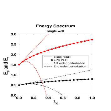
Fig. 3: Energy spectrum.

Fig. 4: $M_{2}=\langle\mathchar 28938\relax|~{}\hat{x}^{2}|\mathchar 28938\relax\rangle$.

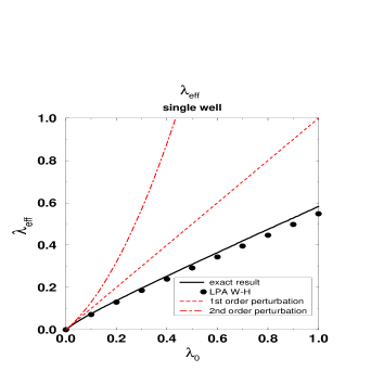
Fig. 5: Effective coupling $\lambda_{\rm eff}$.

The perturbative series of $E_{n}$ is the asymptotic series

$$E_{n}\!=\![n+\frac{1}{2}]+\frac{3}{4}\lambda_{0}[2n^{2}+2n+1]-\frac{1}{8}\lambda_{0}^{2}[34n^{3}+51n^{2}+59n+21]+\cdots.~{}~{}~{}~{}$$ (33)

It diverges even in the weak coupling region. Note that the Borel resummation of the perturbative series works well in this case, and gives quantitatively good values. However, even in the lowest order approximation (LPA), the W-H equation can evaluate the energy spectrum almost perfectly. Therefore, we conclude that the NPRG does sum up all orders of the perturbative series in the correct manner.

We also display the two-point function $M_{2}=\langle\mathchar 28938\relax|~{}\hat{x}^{2}|\mathchar 28938\relax\rangle$ in Figure.5 and the effective four-point coupling constant $\lambda_{\rm eff}$ in Figure.5. In both of these cases as well, the NPRG results give an almost perfect fit.

4.2 Symmetric double-well potential

Next, we consider the $Z_{2}$-symmetric $x\leftrightarrow-x$ double-well potential,

$$V_{0}(x)=\lambda_{0}x^{4}-\frac{1}{2}x^{2}.$$ (34)

In quantum mechanical systems, this $Z_{2}$ symmetry never breaks spontaneously, because the $x$ mode tunnels through the potential barrier, and the ground state is uniquely realized. In fact, in the NPRG evolution of the effective potential, the initial double-well potential finally becomes a single well, and an energy gap (effective mass) arises (Figure.7).

In this system, there is no well-defined perturbation theory. A standard technique to obtain the energy gap $\mathchar 28929\relax E$ is the dilute gas instanton calculation. This is a semi-classical method based on the one-instanton solutions

$$x_{\rm cl}(\tau)=\pm\frac{1}{2\sqrt{\lambda_{0}}}\tanh\frac{(\tau-\tau_{0})}{\sqrt{2}}.$$ (35)

The one-instanton contribution to the partition function $Z$ is

$$Z\simeq Te^{-S\left[x_{\rm cl}\right]}\sqrt{\frac{S\left[x_{\rm cl}\right]}{2\pi}}\left\{\frac{\det^{\prime}\left(\left.\frac{\delta^{2}S}{\delta x^{2}}\right|_{x=x_{\rm cl}}\right)}{\det\left(\left.\frac{\delta^{2}S}{\delta x^{2}}\right|_{x=\pm\frac{1}{2\sqrt{\lambda_{0}}}}\right)}\right\}^{-1/2}\equiv T\frac{\mathchar 28929\relax_{0}}{2},$$ (36)

where $T$ is an imaginary time volume. Assuming that instantons do not interact with each other, we can evaluate the multi-instanton contribution to $Z$ (the dilute gas instanton approximation), and we obtain the energy gap

$$\mathchar 28929\relax E=\mathchar 28929\relax_{0}=2\sqrt{\frac{2\sqrt{2}}{\pi\lambda_{0}}}e^{-\frac{1}{3\sqrt{2}\lambda_{0}}},$$ (37)

which has the structure of an essential singularity originating from the one-instanton action. The singularity coefficient obtained from the instanton method is known to be exact in the vanishing $\lambda_{0}$ limit.[19]

Fig. 6: Flow of the potential.

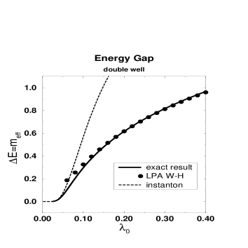
Fig. 7: Energy gap estimates.

Fig. 8: $M_{2}=\langle\mathchar 28938\relax|~{}\hat{x}^{2}|\mathchar 28938\relax\rangle$.

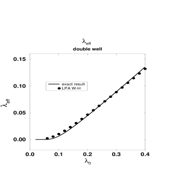
Fig. 9: Effective coupling $\lambda_{\rm eff}$.

In Figure.7 we display the energy gap evaluated using various methods. The NPRG results are very good in the strong coupling region, while the perturbation cannot be applied in this double-well system, and the dilute gas instanton method is not at all effective, because it is valid only in the very weak coupling region. Therefore, the NPRG method should provide a powerful tool for the analysis of tunneling, at least in such regions. However, our NPRG results deviate from the exact values as $\lambda_{0}\to 0$, which corresponds to a very deep well. Because the $\beta$-function becomes singular in this region, the NPRG results become unreliable. We believe that the cause of the difficulty is the LPA approximation scheme that we adopt. It is important to note that the respective coupling regions in which the LPA W-H equation and the dilute gas instanton work well are separated, and therefore these two methods should be regarded as complementary.[10, 20]

We display the two-point function $M_{2}=\langle\mathchar 28938\relax|~{}\hat{x}^{2}|\mathchar 28938\relax\rangle$ in Figure.9 and the effective four-point coupling $\lambda_{\rm eff}$ in Figure.9. As in the case of the energy gap, the NPRG results are excellent here, except in the extremely weak coupling region.

4.3 Flow diagrams

We now more carefully consider the difficulty arising in the weak coupling region for the double-well potential. We employ the operator expansion (12) and investigate the flows of the dimensionless coupling constants $\hat{a}_{n}\equiv a_{n}\mathchar 28931\relax^{-\frac{n+2}{2}}$. The flow diagrams elucidate the phase structure of the system. We display the flow diagrams for the $N=4,6,10$ truncated potentials (Figure.11, Figure.11, Figure.13) and for the potential without an operator expansion (Figure.13).

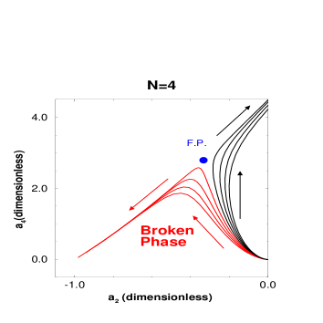
Fig. 10: $N=4$ truncation.

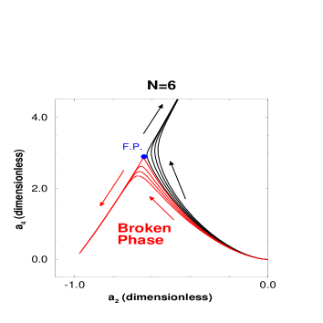
Fig. 11: $N=6$ truncation.

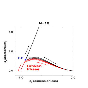
Fig. 12: $N=10$ truncation.

Fig. 13: No truncation.

These flow diagrams reveal that the phase structure of the theory with a truncated potential ($N=4,6,10$) is somewhat strange. As mentioned above, there is no spontaneous symmetry breaking in these quantum mechanical systems. When we truncate the potential as in (12), there appears a non-actual fixed point and false broken phases (Figures 11, 11 and 13). The flow starting from the weak coupling region ($\lambda_{0}\to 0$ i.e. $\hat{a_{4}}\to 0$) tends to be captured by the false broken phase, and we cannot obtain the correct result $m^{2}_{\rm eff}>0$. The region of the false broken phase becomes smaller as $N$ becomes larger, and then for the LPA exact (no truncation) calculation, the false broken phase disappears (Figure.13). However, even in the no truncation case, we cannot obtain reliable results for the flows that start from the weak coupling region, because singular behavior of the flow in the region near $\hat{a}_{2}=-1$ leads to large numerical errors. The results for the LPA W-H equation in Figure.7 were obtained from numerical integration of the partial differential equation without any truncation.[21]

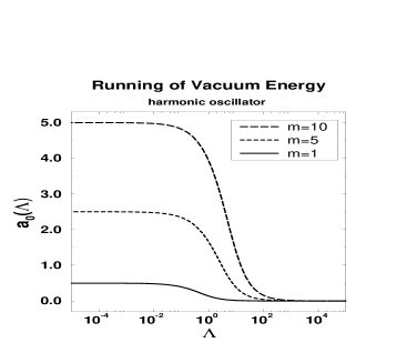
Fig. 1: Running of $a_{0}$.

 

4.4 Other methods

The NPRG equation we employ here is that with the local potential approximation. The results in the weak coupling region can be improved by upgrading the approximation. The LPA is the lowest order of the derivative expansion, and a higher-order calculation can be carried out.[22] In this quantum mechanical system, the second-order calculation of the Legendre flow equation does not improve the weak coupling results.[23] However, an analysis using the proper time renormalization group improves the LPA results considerably.[24] Also, although it differs from the NPRG methods in its formulation, the density matrix renormalization group is useful for this system.[25] We exhibit in Figure.Non-Perturbative Renormalization Group Analysis in Quantum Mechanics the results for the energy gap obtained with various renormalization group approaches.

4.5 Asymmetric double-well potential

We proceed to consider the $Z_{2}$-asymmetric double-well potential

$$V_{0}(x)=~{}~{}\lambda_{0}x^{4}-\frac{1}{2}x^{2}+h_{0}x,$$ (38)

where the linear term $h_{0}x$ breaks the $Z_{2}$ symmetry explicitly. In this system there are a stable minimum and an unstable minimum.

How do we deal with the effect of such an asymmetric term? The NPRG method can treat this system in a manner that is quite similar to that for the symmetric system; it just changes the initial potential, while the LPA W-H equation does not change. Furthermore, when we apply the operator expansion (12), the situation becomes even simpler. The additional $h_{0}x$ term does not affect the running of other coupling constants, because the term

$$\int d\tau\!~{}h_{0}x(\tau)=h_{0}x(E=0),$$ (39)

consists entirely of the zero energy mode, and generates no quantum corrections. Therefore, the NPRG equations for the coupling constants are the same as those in the symmetric case.

By contrast, the standard instanton method cannot be applied to such an asymmetric system, because the term $\left.\frac{\delta^{2}S}{\delta x\delta x}\right|_{x=x_{\rm cl}}$ in (36) has a negative eigenvalue in this case. For actually unstable systems, this negative eigenvalue is converted to a decay rate for the system. This is a typical prescription for the ‘bounce solution’ calculation. However, in the case of the bare potential (34), the true vacuum of the system is stable. The existence of a negative eigenvalue in actually stable systems is known as the problem of a fake instability. To overcome this problem, the valley method has been developed recently.[30, 31] It is a generalization of the instanton method that is based on the valley structure in the configuration space.

As shown in Figure.16, an asymmetric bare potential leads to an asymmetric effective potential. We show in Figure.16 results for the energy gap in the cases of three values of $h_{0}$, from bottom to top, $h_{0}=0.02,\!~{}0.2,\!~{}0.4$. For any value of $h_{0}$, in the $\lambda_{0}\to 0$ limit, $\mathchar 28929\relax E$ approaches $\sqrt{2}$. This is because in this limit the asymmetric double well approaches a single well. We employ the operator expansion and give the truncation $N=12,14,16$ results. We also plot the results obtained from the valley method with fourth and sixth order perturbations.[32] A complementary relation between the NPRG and the valley method is observed, just as in the case of the symmetric potential.

As mentioned above, since in the $\lambda_{0}\to 0$ limit the potential approaches a single well, if we carry out the operator expansion at the potential minimum $x=x_{\rm min}$, the NPRG equations never become singular even in the $\lambda_{0}\to 0$ region, and we obtain $m_{\rm eff}\simeq\sqrt{2}$. We use this technique for analysis of SUSY QM in the next section.

We display results for other quantities in Figure.18 and Figure.18 for three values of $h_{0}$, from top to bottom, $h_{0}=0.02,\!~{}0.2,\!~{}0.4$. The expectation value of $\hat{x}$, $M_{1}=\langle\mathchar 28938\relax|~{}\hat{x}|\mathchar 28938\relax\rangle$, is shown in Figure.18, and the variance of $\hat{x}$ is shown in Figure.18. The NPRG results appear to be perfect on the strong coupling side, while they are incorrect in the weak coupling region.

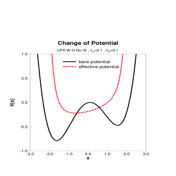
Fig. 15: Flow of the potential.

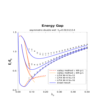
Fig. 16: Energy gap estimates.

Fig. 17: $M_{1}=\langle\mathchar 28938\relax|\hat{x}|\mathchar 28938\relax\rangle$

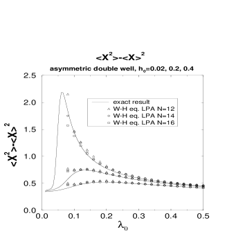
Fig. 18: $\langle\mathchar 28938\relax|\hat{x}^{2}|\mathchar 28938\relax\rangle_{c}$

5 Applications to various quantum systems

We have seen that the NPRG method is very effective in analyses of non-perturbative dynamics in quantum mechanical systems. Here, we apply the NPRG method to more non-trivial quantum systems.

5.1 Supersymmetric quantum mechanics

Here we analyze supersymmetric theory, in which the non-perturbative dynamics of the system are crucial. We consider the SUSY QM theory, which was introduced by Witten as a toy model for dynamical SUSY breaking.[33, 34] The Hamiltonian is given by

$$\hat{H} = \frac{1}{2}\left[\hat{P}^{2}+\hat{W}^{2}(x)+\sigma_{3}\frac{d\hat{W}(x)}{dx}\right]=\left(\matrix{\frac{1}{2}\hat{P}^{2}+\hat{V}_{+}(x)~{}~{}~{}~{}~{}~{}~{}~{}~{}~{}0\cr~{}~{}~{}~{}~{}~{}~{}~{}0~{}~{}~{}~{}~{}~{}~{}~{}~{}~{}~{}~{}\frac{1}{2}\hat{P}^{2}+\hat{V}_{-}(x)}\right),~{}~{}~{}~{}~{}~{}~{}~{}$$ (40)

$$\hat{V}_{\pm}(x) \equiv \frac{1}{2}\hat{W}^{2}(x)\pm\frac{1}{2}\frac{d\hat{W}(x)}{dx},$$ (41)

where $\hat{W}(x)$ is called the SUSY potential. We define the super charges

$$\hat{Q}_{1} = \frac{1}{2}(\sigma_{1}\hat{P}+\sigma_{2}\hat{W}(x)),$$ (42)

$$\hat{Q}_{2} = \frac{1}{2}(\sigma_{2}\hat{P}-\sigma_{1}\hat{W}(x)),$$ (43)

and the Hamiltonian is written as

$$\hat{H}=\{\hat{Q}_{1},\hat{Q}_{1}\}=\{\hat{Q}_{2},\hat{Q}_{2}\}.$$ (44)

This ensures that the vacuum energy is always non-negative:

$$E_{0}=\langle\mathchar 28938\relax|\hat{H}|\mathchar 28938\relax\rangle=2\left\|\hat{Q}_{1}|\mathchar 28938\relax\rangle\right\|^{2}=2\left\|\hat{Q}_{2}|\mathchar 28938\relax\rangle\right\|^{2}\geq 0.$$ (45)

The vacuum energy $E_{0}$ is the order parameter of dynamical SUSY breaking; that is,

$$E_{0}=0\quad\Rightarrow ~{}~{}~{}\hat{Q}_{1}|\mathchar 28938\relax\rangle=0,~{}\hat{Q}_{2}|\mathchar 28938\relax\rangle=0\qquad{\rm unbroken~{}~{}SUSY},$$

$$E_{0}>0\quad\Rightarrow ~{}~{}~{}\hat{Q}_{1}|\mathchar 28938\relax\rangle\neq 0,~{}\hat{Q}_{2}|\mathchar 28938\relax\rangle\neq 0\qquad{\rm broken~{}~{}SUSY}.$$

Furthermore, the perturbative corrections to $E_{0}$ are vanishing for any order of the perturbation. This is known as the non-renormalization theorem. In fact, with the SUSY potential $W(x)=gx^{2}-x$, the potential $V_{+}(x)$ becomes

$$V_{+}(x)=~{}~{}\frac{1}{2}g^{2}x^{4}-gx^{3}+\frac{1}{2}x^{2}+gx-\frac{1}{2}.$$ (46)

The perturbative corrections to the energy spectrum are calculated as

$$E_{n}=n + \frac{3}{8}g^{2}[2n^{2}+2n+1]-\frac{3}{8}g^{2}[10n^{2}+2n+1]$$ (47)

$$- \frac{1}{32}g^{4}[34n^{3}+51n^{2}+59n+21]+\cdots.$$

These corrections to $E_{0}$ are canceled out at each order of $g$, and thus there are no perturbative corrections. Hence, a non-vanishing $E_{0}$ is realized only through non-perturbative effects caused by the essential singularity at the origin of the coupling constant.

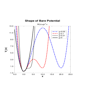
Fig. 19: Bare potentials.

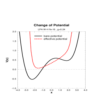
Fig. 20: Potential flow.

We analyze this system using the LPA W-H equation with $N=16$ for the operator expansion.[10] We calculate the effective potential for a wide range of values of the parameter $g$. The case of vanishing $g$ corresponds to the harmonic oscillator with a constant term $-\frac{1}{2}$, and SUSY does not break in this case ($E_{0}=\frac{1}{2}-\frac{1}{2}=0$). However, SUSY is dynamically broken for any non-vanishing $g$. Note that for small $g$, the bare potential is an asymmetric double-well, while for $g>\sqrt[4]{\frac{1}{108}}\simeq 0.31$, it is a single-well, and quantum tunneling is irrelevant (Figure.20). For any value of $g$, the minimum of the bare potential $V_{+}$ is at $x=0$. Figure.20 displays the result for $g$=0.24, where the effective potential evolves into a convex form, and its minimum turns out to be positive; that is, our NPRG method gives a positive $E_{0}$ correctly, and describes the dynamical SUSY breaking.

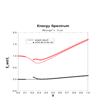
Fig. 21: Energy spectrum.

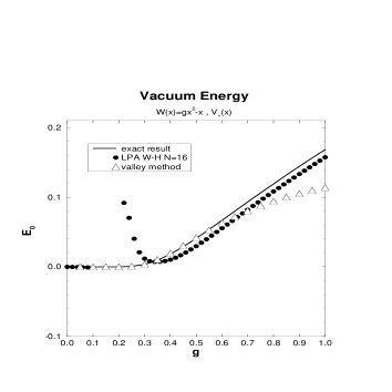
Fig. 22: NPRG and valley method.

As is shown in Figure.22, the NPRG results are excellent in the weak coupling region and strong coupling region, but not in the region where the bare double-well potential becomes deep. In this intermediate region ($0.1\raisebox{0.86108pt}{$\ <\kern-10.50005pt\raisebox{-4.73611pt}{$\sim$}\ $}g\raisebox{0.86108pt}{$\ <\kern-10.50005pt\raisebox{-4.73611pt}{$\sim$}\ $}0.2$), we cannot obtain reliable results because of large numerical errors, while the valley method works very well, as shown in Figure.22. The valley method evaluates the ground state energy as $E_{0}=\frac{1}{2\pi}e^{-\frac{1}{3g^{2}}}$ and reproduces the exact value in the weak coupling region.[31] However, it does not work in the strong coupling region ($g>0.31$), where the valley instanton is no longer a good approximate solution of the valley equation. Again, we find that the two methods are complementary.

5.2 Two particle systems

Next, we apply the NPRG method to quantum many particle systems. As the simplest system, we analyze two particle ($\varphi_{1},\varphi_{2}$) dynamics with the following potential $V_{0}(\varphi_{1},\varphi_{2})$:

$$V_{0}(\varphi_{1},\varphi_{2})=-\frac{1}{2}\varphi^{2}_{1}+\lambda_{0}\varphi_{1}^{4}-\frac{1}{2}\varphi_{2}^{2}+\lambda_{0}\varphi_{2}^{4}+F(\varphi_{1},\varphi_{2}).$$ (48)

Without the interaction $F(\varphi_{1},\varphi_{2})$ between the two particles, the four degenerate ground states are mixed by tunneling, splitting into three $\varphi_{1}\leftrightarrow\varphi_{2}$ symmetric states and one anti-symmetric state. For the interaction $F(\varphi_{1},\varphi_{2})$, we now choose $\varphi_{1}\leftrightarrow\varphi_{2}$ symmetric interactions and investigate how this interaction affects the energy levels of three symmetric states.

The LPA W-H equation for two particles is written

$$\mathchar 28931\relax{\partial V_{\mathchar 28931\relax}\over\partial\mathchar 28931\relax}=-\frac{1}{2\pi}~{}\!\mathchar 28931\relax~{}\!{\rm Tr}\log\left(\delta_{ab}+{\partial^{2}{V}_{\mathchar 28931\relax}\over\partial\varphi_{a}\partial\varphi_{b}}\right),$$ (49)

where “Tr” represents the trace over the subscripts $a,b$ which correspond to the two particles. We consider three types of interactions,

$$F(\varphi_{1},\varphi_{2})=C\varphi_{1}\varphi_{2}~{},~{}C_{2}(\varphi_{1}-\varphi_{2})^{2}~{},~{}C_{4}(\varphi_{1}-\varphi_{2})^{4}.$$ (50)

In the cases of the second and third types, for $C_{2},C_{4}>0$ the interaction is attractive, and for $C_{2},C_{4}<0$ it is repulsive. Since we now treat only the ($\varphi_{1}\leftrightarrow\varphi_{2}$) state, it is convenient to convert the variables from ($\varphi_{1},\varphi_{2}$) to ($x_{1},x_{2}$) as follows:

$$\left(\matrix{x_{1}\cr x_{2}}\right)=\frac{1}{\sqrt{2}}\left(\matrix{1-1\cr 1~{}~{}~{}~{}1}\right)\left(\matrix{\varphi_{1}\cr\varphi_{2}}\right).$$ (51)

The LPA W-H equation for $(x_{1},x_{2})$ has the same form as (49). The lowest energy splitting for symmetric state, $\mathchar 28929\relax E=E_{1}-E_{0}$, is expressed in terms of the effective mass of $x_{2}$. Of course, in the $C=0$ case, this is equal to the effective mass in one particle system.

The bare potentials are written, corresponding to (50), as

$$V_{0}(x) = \frac{1}{2}(-1-C)x^{2}_{1}+\frac{\lambda_{0}}{2}x_{1}^{4}+\frac{1}{2}(-1+C)x_{2}^{2}+\frac{\lambda_{0}}{2}x_{2}^{4}+3\lambda_{0}x_{1}^{2}x_{2}^{2},$$ (52)

$$V_{0}(x) = \frac{1}{2}(-1+4C_{2})x^{2}_{1}+\frac{\lambda_{0}}{2}x_{1}^{4}-\frac{1}{2}x_{2}^{2}+\frac{\lambda_{0}}{2}x_{2}^{4}+3\lambda_{0}x_{1}^{2}x_{2}^{2},$$ (53)

$$V_{0}(x) = -\frac{1}{2}x^{2}_{1}+\left(\frac{\lambda_{0}}{2}+4C_{4}\right)x_{1}^{4}-\frac{1}{2}x_{2}^{2}+\frac{\lambda_{0}}{2}x_{2}^{4}+3\lambda_{0}x_{1}^{2}x_{2}^{2}.$$ (54)

We analyze these systems for small $C,C_{2}$ and $C_{4}$. We set $\lambda_{0}=0.2$, which is in the parameter region where the NPRG works perfectly in previous analyses. The LPA W-H equation was solved numerically using the operator expansion with $N=12$. We also calculated $\mathchar 28929\relax E$ from the first order perturbation theory with one particle Schrödinger wave functions.

The results for small $C,C_{2}$ and $C_{4}$ are shown in Figures 23, 25 and 25. We see that the NPRG results and the Schrödinger wave function results are almost the same in these small interaction regions. These results indicate that an attractive interaction ($C_{2},C_{4}>0$) causes $\mathchar 28929\relax E$ to decrease, and a repulsive interaction ($C_{2},C_{4}<0$) causes it to increase.

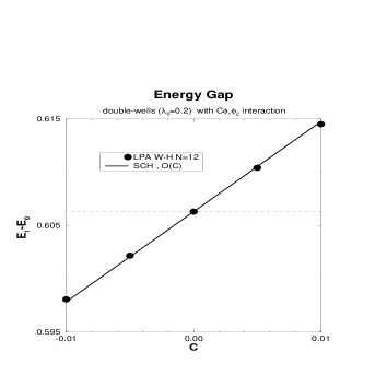
Fig. 23: Linear interaction.

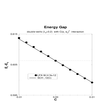
Fig. 24: Quadratic interaction.

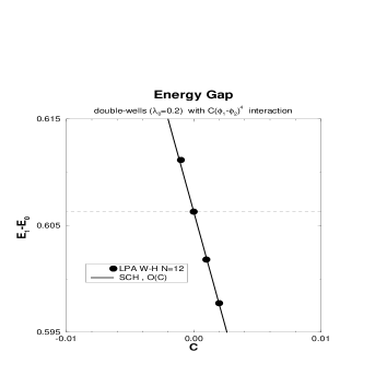
Fig. 25: Quartic interaction.

Here we have shown that for multi-particle systems with interactions, the NPRG method can be applied equally without any change of formulation. We are now carrying out calculations to obtain non-trivial relations between particle interactions and tunneling enhancement/suppression. These results will be reported elsewhere.

6 Summary and Outlook

We have applied the NPRG method to various quantum systems and used it to analyze non-perturbative physics. Even in the first stage of approximation, LPA, we successfully evaluated the non-perturbative quantities that should be given by the summation of all orders of the diverging perturbative series. We also found that for non-perturbative quantities characterized by an essential singularity, the LPA W-H equation again works very well in the region where the instanton-type method breaks down, i.e. the strong coupling region. However, NPRG is not effective in the weak coupling region, due to large numerical errors. In these regions, the approximation used to solve the NPRG equation should be improved in order to obtain correct results. To summarize, the NPRG method and the instanton (or valley) method play complementary roles. Also, from a practical point of view, the NPRG method is a useful new tool for analysis of various quantum systems in a wide parameter region. We have obtained good non-perturbative results for SUSY QM. We also showed that interacting quantum particles can be treated in a similar way.

In the flow diagrams, we observed singular behavior in the small coupling region, and found that it becomes more singular under low-order truncation of the operator expansion. The origin of the difficulty which we encounter in our NPRG analysis resides in the approximation scheme we employed. We must develop ‘better’ approximations, which may depend on the individual systems under study. We also need to study in detail how to extract physical information from the effective potential and the effective action.

A First Pole Dominance

Here we confirm the first pole dominance in the two-point function of anharmonic oscillators. In the local potential approximation, the two-point function is given by following

$$\sum_{n=1}^{\infty}\frac{D_{n}}{E^{2}+(E_{n}-E_{0})^{2}} \stackrel{{\scriptstyle LPA}}{{=}} \frac{1}{E^{2}+m^{2}_{\rm eff}}.$$

This substitutes one pole for an infinite number of poles. Therefore, if the multi-pole contribution becomes significant, the correspondence (25) must be wrong.

Fig. 26: $D_{1}$ for single well potential.

Fig. 27: $D_{1}$ for double well potential.

We evaluated the first pole coefficient $D_{1}$ for a single-well (32) and a double-well (34) by solving the Schrödinger equation numerically. The results are displayed in Figures 27 and 27.

We should note that the relation $\sum_{n}D_{n}=1$ always holds. For the single-well potential, the first pole dominates almost completely. This corresponds to the fact that the results obtained with the LPA W-H equation reproduce the correct results. On the other hand, for the double-well potential, the first pole dominance begins to disappear in the region near $\lambda_{0}=0.1-0.15$, where the results obtained with the LPA W-H equation become poor.

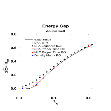
Fig. 14: Various RG results.

References

- [1] K. G. Wilson and J. B. Kogut, Phys. Rep. 12 (1974), 75.
- [2] K.-I. Aoki, Prog. Theor. Phys. Suppl. No.131 (1998), 129.
- [3] T. R. Morris, Prog. Theor. Phys. Suppl. No.131 (1998), 395.
- [4] D.-U. Jungnickel and C. Wetterich, Prog. Theor. Phys. Suppl. No.131 (1998), 495.
- [5] The Exact Renormalization Group, Proceedings of the First Conference on the Exact Renormalization Group (World Scientific, Singapore, 1999).
- [6] K.-I. Aoki, Int. J. Mod. Phys. B 14 (2000), 1249.
- [7] C. Bagnuls and C. Bervillier, Phys. Rep. 348 (2001), 91.
- [8] Proceedings of the Second Conference on the Exact Renormalization Group, Int. J. Mod. Phys. A 16 (2001).
- [9] J. Berges, N. Tetradis and C. Wetterich, Phys. Rep. 363 (2002), 223.
- [10] K.-I. Aoki, A. Horikoshi, M. Taniguchi and H. Terao, in The Exact Renormalization Group (World Scientific, Singapore, 1999), 194 ; hep-th/9812050.
- [11] ed. J. C. Le Guillou and J. Zinn-Justin, Large-Order Behaviour of Perturbation Theory (North-Holland, 1990).
- [12] S. Coleman, Aspects of symmetry (Cambridge University Press, 1985).
- [13] H. Kleinert, Path Integrals in Quantum Mechanics Statistics and Polymer Physics (World Scientific, 1995).
- [14] F. Wegner and A. Houghton, Phys. Rev. A 8 (1973), 401.
- [15] A. Hasenfratz and P. Hasenfratz, Nucl. Phys. B 270 (1986), 687.
- [16] M. E. Peskin and D. V. Schroeder, An Introduction to Quantum Field Theory (Addison-Wesley, 1995).
- [17] K.-I. Aoki, K. Morikawa, W. Souma, J.-I. Sumi and H. Terao, Prog. Theor. Phys. 99 (1998), 451.
- [18] C. Wetterich, Phys. Lett. B 301 (1993), 90.
- [19] B. Simon, Ann. Inst. Henri Poincare 38-3 (1983), 295 ; Ann. of Math. 120 (1984), 89 ; Ann. of Phys. 158 (1984), 415.
- [20] P. Gosselin, B. Grosdidier and H. Mohrbach, Phys. Lett. A 256 (1999), 125.
- [21] A. S. Kapoyannis and N. Tetradis, Phys. Lett. A 276 (2000), 225.
- [22] T. R. Morris, Phys. Lett. B 329 (1994), 241.
- [23] K.-I. Aoki and A. Horikoshi, unpublished.
- [24] D. Zappala, Phys. Lett. A 290 (2001), 35.
- [25] M. A. Martin-Delgado, G. Sierra and R. M. Noack, cond-mat/9903100.
- [26] T. Kashiwa, Phys. Rev. D 59 (1999), 085002.
- [27] R. Guida, K. Konishi and H. Suzuki, Ann. of Phys. 241 (1995), 152 ; Ann. of Phys. 249 (1996), 109.
- [28] T. Hatsuda, T. Kunihiro and T. Tanaka, Phys. Rev. Lett. 78 (1997), 3229.
- [29] T. Kunihiro Prog. Theor. Phys. Suppl. No.131 (1998), 459 ; Phys. Rev. D 57 (1998), 2035.
- [30] H. Aoyama, H. Kikuchi, T. Harano, I. Okouchi, M. Sato and S. Wada, Prog. Theor. Phys. Suppl. No.127 (1997), 1.
- [31] H. Aoyama, H. Kikuchi, I. Okouchi, M. Sato and S. Wada Phys. Lett. B 424 (1998), 93 ; Nucl. Phys. B 553 (1999), 644.
- [32] H. Aoyama, private communications.
- [33] E. Witten, Nucl. Phys. B 188 (1981), 513 ; Nucl. Phys. B 202 (1982), 253.
- [34] P. Salomonson and J. W. van Holten, Nucl. Phys. B196 (1982), 509.