Entanglement of two atomic samples by quantum non-demolition measurements.

Abstract

This paper presents simulations of the state vector dynamics for a pair of atomic samples which are being probed by phase shift measurements on an optical beam passing through both samples. We show how measurements, which are sensitive to different atomic components, serve to prepare states which are close to being maximally entangled.

I Introduction

The population of an atomic state $|1\rangle$ can be probed by a phase shift measurement on a field that couples $|1\rangle$ non-resonantly to another atomic state. This implies that for an atomic sample with all atoms populating two long lived states $|1\rangle$ and $|2\rangle$, it is possible to count non-destructively the number $n_{1}$ of atoms in $|1\rangle$. The state vector or density matrix of the sample with, e.g., an initial binomial distribution of populations $n_{1}$ will be modified, as the quantum mechanical uncertainty of the number $n_{1}$ is reduced during the measurement kuz98 ; moelmer99 ; bouchoule02 . This effect has been demonstrated experimentally kuz99 ; Kuz00 , and further theoretical proposals Duan00 have addressed the possibility to entangle pairs of samples by performing joint phase shift measurements, where light is propagated through both samples and thus provides information about total occupancies of various states. In particular it has been possible to prepare EPR-correlated samples juls01 where the entanglement could be experimentally proven by a quantitative test involving spin noise measurements ciracgauss ; simongauss .

The theoretical analysis in Duan00 ; juls01 addresses the behavior of collective atomic spin operators due to their interaction with the field operators (in the Heisenberg picture). Following the analysis in bouchoule02 , in the present paper we present wave function simulations, in which we display how the sequence of photo-detection events gradually modifies the state vector of the samples. The two approaches are of course equivalent, but they may provide different insights, and in addition the present state vector approach does not rely on the atomic operators being approximated by harmonic oscillators, i.e., we can treat cases where the mean polarization changes significantly in the samples, which is not practically possible in the operator formulation.

The paper is organized as follows. In Sec. II, we introduce our physical model for the measurement of optical phase shifts, and we present the formal description of the state vector evolution conditioned on the photo-detection record. In Sec. III, we show results of simulations where the atoms are first all prepared in superposition states of the two internal states prior to detection of the number of atoms in state $|1\rangle$. We show that the resulting state vector is entangled, and we show that a subsequent spin rotation of all atoms followed by new measurements will lead to stronger entanglement. In Sec. IV, we show simulations where the atomic samples are subject to continuous spin rotation during measurement, corresponding to the experimental situation of Ref.juls01 . In Sec. V, we present an analysis and interpretation of the results, and Sec. VI concludes the paper.

II Optical phase shift measurements

In our model we are considering clouds of atoms whose relevant level structure consists of three levels: two degenerate ground states, $\left|1\right\rangle$ and $\left|2\right\rangle$, and an exited state, $\left|3\right\rangle$. We suppose that the only permitted transition is $\left|1\right\rangle\rightarrow\left|3\right\rangle$, excited by the laser beam passing through the cloud and followed by spontaneous decay with emission rate $\gamma$, cf., Fig. 1.

Figure 1: Level structure of the atoms. The states $\left|1\right\rangle$ and $\left|2\right\rangle$ are stable states, $|1\rangle$ is coupled off-resonantly by the probe to the excited state $\left|3\right\rangle$.

Our scheme is based on the detection of photons passing through the clouds. The scheme only requires classical input fields, since the state reduction following every single photodetection event, a posteriori, extracts the effect of the interaction of a single photon with the atomic samples. There are different possibilities to create a detection scheme that measures the population of a single atomic state, or the population difference between two atomic states. One can use light with two polarization components that interact differently with the two internal states, and hence the different phase shifts lead to a polarization rotation signal; or, one can use frequency modulated light, where one frequency component is closer to resonance than the other, and hence a phase difference between the two results from the interaction between the atoms. For ease of presentation, we follow the description in bouchoule02 , and imagine an interferometric setup, where a field is split in two paths, one that interacts with the atomic samples and one that propagates through free space. This experimental set-up is schematically shown in Fig. 2. A phase difference between these two fields due to the atoms can be resolved by the intensities measured by photo-detectors $D_{+}$ and $D_{-}$ in the two output ports of the interferometer. We may enclose the atomic samples in optical cavities to enhance the interaction with the atoms by passing the light through each sample many times. This will also reduce the effect of spontaneous scattering which will hence be omitted from the present analysis. As shown in bouchoule02 wave function simulations can incorporate spontaneous scattering, and it can also be estimated in the operator formulation Duan00 .

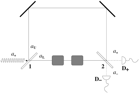
Figure 2: Atoms occupying the internal state $|1\rangle$ in the two samples interact with the light field which is incident from the left in the figure. The phase shift of the light field due to interaction with these atoms is registered by the different photo-currents in the two detectors.

Let us introduce the atomic transition operators $\sigma_{ij}^{n}=\left|i\right\rangle_{n}\!\left\langle j\right|$, where $i(j)=1,2,3$ and $n$ enumerates the atoms. In the dipole and rotating wave approximation, the interaction Hamiltonian is:

$$H_{I}=\sum_{n}g(\sigma_{13}^{n}a_{L}^{{\dagger}}+\sigma_{31}^{n}a_{L})$$ (1)

where $g$ is the atom-photon interaction strength, and $a_{L}$ is the annihilation operator for the field component interacting with the atoms.

If $\Delta$ is the detuning between the light field and the atomic transition frequency $(E_{3}-E_{1})/\hbar$, the second order transition amplitude for the interaction process is:

$$\mathcal{I}_{fi}=\frac{g^{2}\Delta}{\Delta^{2}-\frac{\gamma^{2}}{4}}-i\frac{g^{2}\frac{\gamma}{2}}{\Delta^{2}-\frac{\gamma^{2}}{4}}$$ (2)

where the indices $i$ and $f$ represent the initial and final state of the process, which in our case is the same state of an atom in $|1\rangle$ and one photon of the radiation field.

In the case of off resonant scattering, with $\Delta\gg\gamma$, we get

$$\mathcal{I}_{fi}=\frac{g^{2}}{\Delta}.$$ (3)

which is just the energy shift of state $\left|1\right\rangle$ due to the absorbed and re-emitted photon. Hence, the time evolution of the atom-photon state assumes the form $\left|1\right\rangle\otimes\left|n_{L}=1\right\rangle\stackrel{{\scriptstyle\tau}}{{\longrightarrow}}e^{-i\frac{g^{2}}{\Delta}\tau}\left|1\right\rangle\otimes\left|n_{L}=1\right\rangle$.

Defining $\chi=\frac{g^{2}}{\Delta}$, we can write an effective Hamiltonian describing the interaction between a single mode light field and a gas of $N$ atoms:

$$H_{eff}\equiv\sum_{n}\chi\left|1\right\rangle_{n}\!\left\langle 1\right|a_{L}^{{\dagger}}a_{L}=\sum_{n}\chi\sigma_{11}^{n}a_{L}^{{\dagger}}a_{L}.$$ (4)

By introducing the atomic spin operators for the ground states

$$j_{nz} = \frac{1}{2}\left(\sigma_{22}^{n}-\sigma_{11}^{n}\right)$$ (5)

$$j_{n+} = \frac{1}{2}\sigma_{21}^{n}$$ (6)

$$j_{n-} = \frac{1}{2}\sigma_{12}^{n},$$ (7)

the effective Hamiltonian (4) becomes

$$H_{eff}=\sum_{n=1}^{N}\chi\left(\frac{1}{2}-j_{nz}\right)a_{L}^{{\dagger}}a_{L}.$$ (8)

In an ensemble of atoms, where each atom is initially prepared in the same state, and where the interaction with the surroundings is identically the same for all atoms, the collective atomic state retains the full permutation symmetry, and it is convenient to expand this collective state on eigenstates for the effective collective angular momentum:

$$\left|\Psi\right\rangle=\sum_{M=-J}^{J}\mathcal{A}_{M}\left|J,M\right\rangle,$$ (9)

where $J=\frac{N}{2}$ is the total angular momentum, and $M=\frac{1}{2}\left(n_{2}-n_{1}\right)$ is the eigenvalue of the operator $J_{z}=\sum_{n}^{N}j_{nz}$. Collective raising and lowering operators, and the corresponding cartesian $x$- and $y$- components of the collective angular momentum, are defined as similar sums over all atoms in the sample.

A photon incident on the interferometer splits as a superposition of a photon in the upper path and a photon in the lower path, $\frac{1}{\sqrt{2}}(\left|U\right\rangle_{ph}+\left|L\right\rangle_{ph})$, and the time evolution of the collective atomic state due to the interaction with this photon for a duration $\tau$ is given by

$$\left|\Phi(\tau)\right\rangle_{ph+at} = e^{-i\sum_{n=1}^{N}\chi\left(\frac{1}{2}-j_{nz}\right)a_{L}^{{\dagger}}a_{L}\tau}\frac{1}{\sqrt{2}}(\left|U\right\rangle_{ph}+\left|L\right\rangle_{ph})\otimes\left|\Psi\right\rangle$$ (10)

$$= \sum_{M=-J}^{J}\frac{\mathcal{A}_{M}}{\sqrt{2}}\left(\left|U\right\rangle_{ph}+e^{-i\left(\frac{N}{2}-M\right)\chi\tau}\left|L\right\rangle_{ph}\right)\otimes\left|J,M\right\rangle,$$

where $\left(\frac{N}{2}-M\right)=\left(\frac{n_{1}+n_{2}}{2}-\frac{n_{2}-n_{1}}{2}\right)=n_{1}$. Hence, as claimed above, the phase shift of the single photon state $|L\rangle_{ph}$ is proportional to the total population of state $\left|1\right\rangle$.

II.1 Entanglement due to measurement

In bouchoule02 the interaction with a single sample is analyzed in detail, and the possibility to achieve spin squeezing due to the interaction with the atoms is analyzed. We now turn our attention to a system of two atomic ensembles of $N_{1}$ and $N_{2}$ atoms, respectively. Within each sample we assume permutation symmetry among the atoms, i.e., each sample is represented by the collective spin states, introduced above.

The state vector of the samples can be expanded on product state wave functions of the two ensembles

$$\left|\Psi\right\rangle=\sum_{M_{1},M_{2}}\mathcal{A}_{M_{1},M_{2}}\left|M_{1},M_{2}\right\rangle,$$ (11)

where $|M_{1},M_{2}\rangle\equiv|J_{1}=N_{1}/2,M_{1}\rangle\otimes|J_{2}=N_{2}/2,M_{2}\rangle$, and where we assume an initial product state $\mathcal{A}_{M_{1},M_{2}}=\mathcal{A}_{M_{1}}\mathcal{A}_{M_{2}}$ before we submit the system to the incident field. The photon interacts with each of the ensembles in the lower arm of the interferometer, and the state of the system after the interaction, but before the photo-detection, is

$$\left|\Phi(\tau)\right\rangle_{ph+at}=\sum_{M_{1},M_{2}}\mathcal{A}_{M_{1},M_{2}}\left(\frac{\left|U\right\rangle_{ph}+e^{-i\left[\frac{N_{1}+N_{2}}{2}-\left(M_{1}+M_{2}\right)\right]\chi\tau}\left|L\right\rangle_{ph}}{\sqrt{2}}\right)\otimes\left|M_{1},M_{2}\right\rangle$$ (12)

The detectors $D_{+}$ and $D_{-}$ click, when they detect a photon in one of the states $\left|\pm\right\rangle_{ph}=\frac{1}{\sqrt{2}}\left(\left|U\right\rangle_{ph}\pm\left|L\right\rangle_{ph}\right)$, and associated with this detection event the photon is destroyed by the action of one of the annihilation operators $a_{+}$ and $a_{-}$. It is thus useful to rewrite the photon-atom state explicitly in terms of the two components distinguished by the photodetectors:

$$\left|\Phi(\tau)\right\rangle_{ph+at} = \sum_{M_{1},M_{2}}\mathcal{A}_{M_{1},M_{2}}\left(\frac{1+e^{-i\left[\frac{N_{1}+N_{2}}{2}-\left(M_{1}+M_{2}\right)\right]\chi\tau}}{2}\right)\left|M_{1},M_{2}\right\rangle\otimes\left|+\right\rangle_{ph}$$ (13)

$$+\sum_{M_{1},M_{2}}\mathcal{A}_{M_{1},M_{2}}\left(\frac{1-e^{-i\left[\frac{N_{1}+N_{2}}{2}-\left(M_{1}+M_{2}\right)\right]\chi\tau}}{2}\right)\left|M_{1},M_{2}\right\rangle\otimes\left|-\right\rangle_{ph}.$$

The probabilities that the photon is detected in state $\left|+\right\rangle_{ph}$ or in state $\left|-\right\rangle_{ph}$, are

$$\pi_{+} = \sum_{M_{1},M_{2}}\left|\mathcal{A}_{M_{1},M_{2}}\right|^{2}$$ (14)

$$\times \cos^{2}{\left[\left(\frac{N_{1}+N_{2}}{4}-\frac{M_{1}+M_{2}}{2}\right)\chi\tau\right]},$$

$$\pi_{-} = \sum_{M_{1},M_{2}}\left|\mathcal{A}_{M_{1},M_{2}}\right|^{2}$$ (15)

$$\times \sin^{2}{\left[\left(\frac{N_{1}+N_{2}}{4}-\frac{M_{1}+M_{2}}{2}\right)\chi\tau\right]}.$$

Thus, after the detection of a photon, the state of the two ensembles of atoms is projected, with probability $\pi_{+}$ and $\pi_{-}$ respectively, into one of the following states

$$\left|\Psi\right\rangle_{+} = \frac{1}{\sqrt{C_{+}}}\sum_{M_{1},M_{2}}\frac{\mathcal{A}_{M_{1},M_{2}}}{2}$$ (16)

$$\times \left(1+e^{-i\left[\frac{N_{1}+N_{2}}{2}-\left(M_{1}+M_{2}\right)\right]\chi\tau}\right)\left|M_{1},M_{2}\right\rangle$$

$$\left|\Psi\right\rangle_{-} = \frac{1}{\sqrt{C_{-}}}\sum_{M_{1},M_{2}}\frac{\mathcal{A}_{M_{1},M_{2}}}{2}$$ (17)

$$\times \left(1-e^{-i\left[\frac{N_{1}+N_{2}}{2}-\left(M_{1}+M_{2}\right)\right]\chi\tau}\right)\left|M_{1},M_{2}\right\rangle\!,$$

where $C_{\pm}$ are normalization factors. From Eqs. (16) and (17) we observe the entanglement between the two atomic ensembles emerge.

The detection procedure, and the corresponding wave function updating, is repeated for a number $N_{ph}$ of photons, being detected one at a time. Hence, by defining the following entangling factors

$$\mathcal{F}_{\pm}(M_{1}+M_{2})=\left(\frac{1\pm e^{-i\left[\frac{N_{1}+N_{2}}{2}-\left(M_{1}+M_{2}\right)\right]\chi\tau}}{2}\right),$$ (18)

after $N_{ph}$ detected photons, of which $N_{+}$ are detected by $D_{+}$ and $N_{-}=N_{ph}-N_{+}$ are detected by $D_{-}$, the state vector of the samples is

$$\left|\Psi\right\rangle_{N_{ph}} = \frac{1}{\sqrt{C}}\sum_{M_{1},M_{2}}\mathcal{A}_{M_{1}}\mathcal{A}_{M_{2}}\left[\mathcal{F}_{+}(M_{1}+M_{2})\right]^{N_{+}}$$ (19)

$$\times\left[\mathcal{F}_{-}(M_{1}+M_{2})\right]^{(N_{ph}-N_{+})}\left|M_{1},M_{2}\right\rangle.$$

The square norm of the entangling factor in equation (19) is

$$\mathcal{B}(M_{12}) = \left[\cos\left(\frac{N-M_{12}}{2}\chi\tau\right)\right]^{2N_{+}}$$ (20)

$$\times\left[\sin\left(\frac{N-M_{12}}{2}\chi\tau\right)\right]^{2(N_{ph}-N_{+})},$$

where $M_{12}=M_{1}+M_{2}$, and where, for simplicity, we assume the same number of atoms in each sample $N=N_{1}=N_{2}$. For large $N_{ph}$ this function is very peaked with maxima at values $M_{12}=\overline{M}$ obeying

$$\tan\left(\frac{N-\overline{M}}{2}\right)\chi\tau=\pm\sqrt{\frac{N_{ph}-N_{+}}{N_{+}}}.$$ (21)

Equation (21) has multiple solutions for $\overline{M}$, due to both the periodicity of the $tan$-function and the double sign in the right hand side, but we can remove this ambiguity in the solutions if we ensure that only a single maximum is compatible with the initial distribution of the two samples in $M_{1}$ and $M_{2}$. Calculating the second derivative of $\mathcal{B}(M_{12})$ around the maximum values, we get an estimate of the width of the peak in $M_{12}$

$$\left.\partial_{M_{12}}^{2}\mathcal{B}(M_{12})\right|_{\tiny{M_{12}=\overline{M}}}=-(\chi\tau)^{2}N_{ph}\mathcal{B}(M_{12}).$$ (22)

If the number of atoms is large enough, we can approximate $\mathcal{B}(M_{12})$ with a Gaussian, and with this approximation we obtain the r.m.s width

$$\Delta M_{12}=\frac{1}{\chi\tau\sqrt{N_{ph}}}.$$ (23)

Thus, the more photons that are detected, the more peaked is the distribution in $M_{12}$.

III Numerical simulation, consecutive measurements of $J_{z1}+J_{z2}$ and $J_{y1}-J_{y2}$

In this section, the detection model described in the previous section will be implemented in a numerical simulation in which the two samples have the same, not very large, number $N$ of atoms and the initial state is the eigenstate of the operator $J_{x1}+J_{x2}$ with eigenvalue $J_{1}+J_{2}=2J=N$, i.e., all the atoms are initially prepared in the superposition state $\frac{1}{\sqrt{2}}(|1\rangle+|2\rangle)$. The corresponding amplitudes in the basis eigenstates of the $z$-component of the collective angular momentum operators $|J,M_{i}\rangle$ are

$$\mathcal{A}_{M_{i}}=\left(\frac{1}{2}\right)^{J}\sqrt{\frac{(2J)!}{(J+M_{i})!(J-M_{i})!}}\;,$$ (24)

where $i=1,2$. Expressed in terms of the number of atoms in state $|1\rangle$ in each sample, $n_{1}^{i}$, the square of the amplitude (24) is $|\mathcal{A}_{M_{i}}|^{2}=\left(\frac{1}{2}\right)^{N}\frac{N!}{(N-n_{1}^{i})!(n_{1}^{i})!}$. This means that in each ensemble the atoms are distributed in state $\left|1\right\rangle$ and $\left|2\right\rangle$ according to a binomial distribution with probability $\frac{1}{2}$.

Beginning with an initial state characterized by amplitudes (24), we proceed with a series of photo detections that project the state of the system according to Eqs. (16) and (17). After a large number of photons $N_{ph}$ has been detected, the uncertainty in $M_{12}$ is reduced, i.e., we are almost in one of the eigenstates of $J_{1z}+J_{2z}$. Fig. 3 shows the behavior of the variance $\Delta^{2}(J_{1z}+J_{2z})$ as a function of the number of detected photons for three different simulation records. It is evident that when the number of detected photons is large enough, $\Delta^{2}(J_{1z}+J_{2z})$ goes to zero, i.e we have a definite value of $\overline{M}=M_{1}+M_{2}$. In the simulations we assume a phase angle $\chi\tau=0.24$. Such a large phase shift on the atomic state due to interaction with a single photon is not realistic in experiments with freely propagating fields. In our simulations a smaller value of $\chi\tau$ just implies that more photons have to be detected to achieve the same reduction in $\Delta^{2}(J_{1z}+J_{2z})$, c.f., (23).

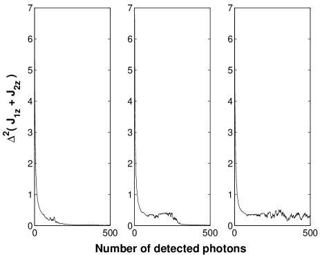
Figure 3: Variance of $J_{1z}+J_{2z}$ as function of the number of detected photons. Each sample consists of 20 atoms in the simulations, and the phase angle $\chi\tau$ per atom and photon is 0.24 in the simulation.

To quantify the entanglement between the two samples we apply the definition by Bennett et al bennett96 of the entanglement between two systems in a pure state $|\Psi\rangle$:

$$\mathcal{E}=Tr(\rho_{1}\log_{2}\rho_{1})=Tr(\rho_{2}\log_{2}\rho_{2}),$$ (25)

where $\rho_{1}=Tr_{2}\left|\Psi\right\rangle\left\langle\Psi\right|$ is the reduced density matrix of system 1. (Similarly for $\rho_{2}$). If $N$ is the number of atoms in each sample, and we restrict ourselves to states which are symmetric under permutations inside samples, the quantity $\mathcal{E}$ takes values between zero for a product state, and $\log_{2}(N+1)$ for a maximally entangled state of the samples.

Fig. 4 shows the behavior of the entropy in three different simulations. The left hand side of each figure, for $N_{ph}<500$ corresponds to the detection, analyzed above. To prove that the samples are entangled and not just classically correlated, in the experiments of juls01 a second observable was introduced, for which the quantum mechanical uncertainty was similarly reduced, and measurements on both sets of observables conclusively demonstrate the entanglement ciracgauss ; simongauss . In our theoretical calculation, we know of course already that the state is entangled, but as we shall see, we can increase the entanglement by taking a second round of measurements.

Thus, after the detection of 500 photons, we apply opposite rotations to the atomic samples, and we proceed with similar measurements as before, which effectively measure $J_{1y}-J_{2y}$ in the non-rotated frame. After the rotations, the full permutation symmetry of the system is broken, i.e the total angular momentum $J^{2}=J_{x}^{2}+J_{y}^{2}+J_{z}^{2}$ is not conserved. The final state of the two samples is still an eigenstate of both $J_{1}^{2}$ and $J_{2}^{2}$, but with different values of the total $J$. Our formalism (25,26) is already prepared to handle that situation, since the basis vectors in the expansion are kept on the form of product states rather than angular momentum coupled states of the two samples.

As illustrated by the right hand parts of the panels in Fig. 4, the entanglement had essentially saturated after the first 500 detection events, but after the rotation, it grows again to saturate, typically, at a higher level. In Fig. 4(a) we show an example of the evolution of the entropy in which the final value ($\mathcal{E}_{N_{ph}}=4.3193$) is very close to that of the maximally entangled state ($\log_{2}(20+1)=4.3923$). In Fig. 4(c), however, we show a case in which the final entropy value is reduced by the second set of rotations. In Sec. V, we shall return to an analysis of these findings. Finally, Fig. 4(d) presents the average of the entropy over 50 simulations.

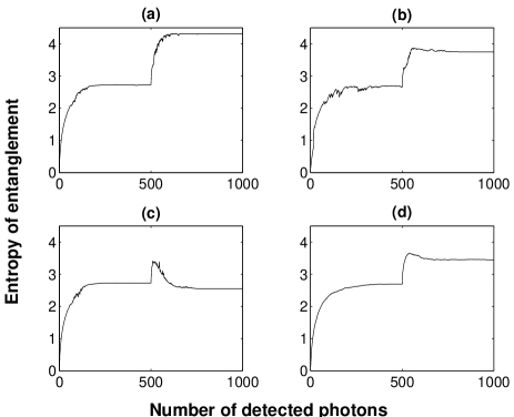
Figure 4: Entanglement of two samples of each $N=20$ atoms. After detection of the first $N_{ph}=500$ photons, the samples are rotated $\pm 90$ degrees in spin space, and the subsequent detection events lead, typically, to further entanglement. Figs. 4 (a-c) show results of three different simulation records, Fig. 4(d) shows the average over 50 such simulations. $\chi\tau=0.24$ as in Fig. 3.

IV Measurements with continuous rotation of spin components

As we just saw that measurements of two different sets of operators typically lead to an increase of the amount of entanglement, it is natural to consider a continuous change between these operators. In fact, in the experimental work by Julsgaard et al juls01 , such a continuous rotation was induced for purely practical reasons (so that the relevant signal could be picked up in the absence of technical noise at a high frequency). In this section we present the results of simulations in which continuous opposite rotations are applied to the atomic spins of the two samples as the photo detection proceeds. If $\mathcal{A}_{M_{1}M_{2}}^{N_{ph}}$ is the wave function amplitude of the system after $N_{ph}$ photo detections, the updated state vector rotated by the angle $\pm\theta$ prior to the subsequent detection is

$$\left|\Psi\right\rangle_{N_{ph}}=\sum_{M^{{}^{\prime}}_{1},M^{{}^{\prime}}_{2}}\sum_{M_{1},M{2}}\mathcal{D}^{J_{1}}_{M_{1}M^{{}^{\prime}}_{1}}\left(\theta\right)\mathcal{D}^{J_{2}}_{M_{2}M^{{}^{\prime}}_{2}}\left(-\theta\right)\mathcal{A}_{M_{1}M_{2}}^{N_{ph}}\left|M^{{}^{\prime}}_{1},M^{{}^{\prime}}_{2}\right\rangle,$$ (26)

where $D^{J_{i}}_{M_{i}M^{{}^{\prime}}_{i}}\left(\theta\right)=\left\langle M_{i},J_{i}\right|e^{-iJ_{ix}(\theta)}\left|J_{i},M_{i}^{{}^{\prime}}\right\rangle$ is the rotation matrix element for sample $i=1,2$. The wave function updating algorithm has the same structure as described in section II. In a realistic experimental situation, one would detect photons according to a Poisson process, and with a constant rotation frequency, induced, e.g., by application of opposite DC magnetic fields onto the atoms, this would lead to small rotation angles with an exponential distribution law. For simplicity, however, we apply the same small rotation angle $\theta$ between each detection event.

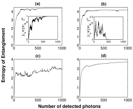
Figure 5: Entanglement of atomic samples with 20 atoms. The spins are rotated in opposite directions around the $x$-axis by the angle $\theta=\frac{\pi}{5}$ after each detection event. Insets (a) and (b) show the evolution of the overlap $|\left\langle\Psi_{0}\right|\Psi\rangle_{N_{ph}}|^{2}$ between the state of the samples and the maximally entangled state (See section (V)). In (a) $\left|\Psi\right\rangle_{N_{ph}}$ converges towards $\left|\Psi_{0}\right\rangle$ and further detections have no effect on the state vector. In (b) the state gradually gets rid of its component along $\left|\Psi_{0}\right\rangle$, and it subsequently evolves in the orthogonal subspace of $\left|\Psi_{0}\right\rangle$. In (c) is shown a record where the entanglement is smaller than in the simulations in (a) and (b), and in (d) is shown the average over 50 simulations.

In Fig. 5 we show realizations of the detection scheme with small rotations. The rotation angle between subsequent photodetection events is $\theta=\frac{\pi}{5}$. Fig. 5(a) shows a case where the entropy evolves to the maximum value: $\mathcal{E}_{N_{ph}}=4.3923$. In Fig. 5(b) and 5(c) we present ’typical’ and ’worst case’ results of the simulations, while in Fig. 5(d) we provide the average over 50 simulations.

We observe in these figure that compared to the results shown in the previous section, there is a faster increase of the entanglement towards an almost constant level, which varies from one simulation to the other.

V Analysis and interpretation

In order to interpret the results obtained in the previous sections, let us first address the achievements of probing two operators rather than a single one. The improvement is quite easily understood, if one notes that the detection of $J_{z1}+J_{z2}$ effectively produces an approximate eigenstate of this operator. This state has amplitudes on different $M_{1}$ and $M_{2}$ states with $M_{1}+M_{2}$ fixed by the measured value, but the eigenspace is degenerate, and the amplitudes are simply proportional to the ones in the initial state. Due to the initial binomial distribution on $M_{1}$ and $M_{2}$, the distribution over, e.g., $M_{1}$ will therefore have a width of approximately $\sqrt{N}$. The reduced density matrix has the corresponding number of non-vanishing populations, suggestive of $\mathcal{E}\sim\log_{2}\sqrt{N}=0.5\log_{2}N$, half of the maximal value. This argument accounts for the first plateau reached in Fig. 4.

The measurement of the $z$-components causes a broadening of the distribution on $J_{y}$ eigenstates beyond the initial distribution, which was also binomial in that basis. The subsequent measurement of $J_{y1}-J_{y2}$ will produce a state with $M_{1y}-M_{2y}$ fixed by the measurement, but within the degenerate space of states with this fixed value the distribution on $M_{1y}$ of the reduced density matrix is broader than $\sqrt{N}$, and the entanglement is correspondingly larger. This accounts for the increase of entanglement seen in most simulations.

For large collections of atoms with large mean values of the collective $J_{x}$ operators, the orthogonal spin components $J_{z}$ and $J_{y}$ are well approximated by effective position and momentum operators, and for two particles, the pair of combinations of position and momentum operators $x_{1}+x_{2}$ and $p_{1}-p_{2}$ commute, i.e., they can both be measured with high precision. But, this is not an exact replacement, and in our simulations with fewer atoms, we see significant deviations from this picture. The commutator of $J_{z1}+J_{z2}$ and $J_{y1}-J_{y2}$ is proportional to the operator $J_{x1}-J_{x2}$ which does not vanish, and in general, measurements sensitive to one of these operators are complimentary to measurements sensitive to the other one. It is possible, however, to find a single joint eigenstate of the operators wang02 :

$$(J_{1x}-J_{2x})|\Psi_{0}\rangle = 0,$$ (27)

$$(J_{1y}-J_{2y})|\Psi_{0}\rangle = 0.$$ (28)

Rewriting these equations as

$$(J_{1+}-J_{2+})|\Psi_{0}\rangle = 0,$$ (29)

$$(J_{1-}-J_{2-})|\Psi_{0}\rangle = 0,$$ (30)

it is easy to check that the solution is the maximally correlated state

$$|\Psi_{0}\rangle=\frac{1}{\sqrt{2J+1}}\sum_{M=-J}^{J}|M,-M\rangle$$ (31)

Note that $|\Psi_{0}\rangle$ also satisfies $(J_{1z}+J_{2z})|\Psi_{0}\rangle=0$, and in fact, all spin components have vanishing mean values in this state.

When we simulate the detection of phase shifts proportional to $J_{1z}+J_{2z}$ and $J_{1y}-J_{2y}$, or combinations of these operators, there is a chance, that the state vector is gradually projected onto $|\Psi_{0}\rangle$, and this state is unaffected by all future photodetection events. Indeed, in some of our simulation records, we precisely see the robust generation of the maximally entangled state, cf., Fig. 5(a).

If one has not collapsed into $|\Psi_{0}\rangle$ after a large number of photons have been detected, the state vector is instead orthogonal to that state, and one will never arrive at the maximally entangled state. The insets of the figures show the wave function overlap with $|\Psi_{0}\rangle$, and in all simulations this quantity converges to either unity, as in Fig. 5(a), or to zero, as in Fig. 5(b). The overlap between $|\Psi_{0}\rangle$ and our initial state suggests that in one out of $N+1$ realizations of the experiment, one should produce that particular state, and this is confirmed by our simulations.

There are no other joint eigenstates of the pair of collective operators, and hence state vectors orthogonal to $|\Psi_{0}\rangle$ do not evolve into any specific state: measurements on the system have different outputs which affect the state vector in different ways. We do note, however, that fairly strong entanglement is observed in many realizations, and that this entanglement is almost constant over time. This is suggestive of families of states with relatively well defined values of the operators $J_{1z}+J_{2z}$ and $J_{1y}-J_{2y}$, which is allowed by Heisenberg’s uncertainty relation as long as the expectation value of the operator $J_{1x}-J_{2x}$ is small. Figs. 6-8 present the three mean values of $J_{1x}-J_{2x}$, $J_{1y}-J_{2y}$ and $J_{1z}+J_{2z}$ for the evolution leading to the maximally entangled state, a very entangled state and a less entangled state studied in Fig. 5 (a-c). The picture is precisely as expected: the maximally entangled state does not change with time and the mean values vanish forever, a strongly entangled non-stationary state performs almost regular oscillations in a limited part of Hilbert space restricting the mean values to a similar small oscillatory behaviour, and states with little entanglement show more dramatic time dependence and the mean values explore a wide range of values. It was unexpected that the non-maximally entangled states seem to be consistently much entangled or little entangled for long detection sequences. Further studies of this dynamics would be very interesting.

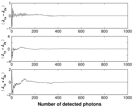
Figure 6: Evolution of $\langle J_{1x}-J_{2x}\rangle$, $\langle J_{1y}-J_{2y}\rangle$ and $\langle J_{1z}+J_{2z}\rangle$ corresponding to the simulation shown in Fig. 5(a).

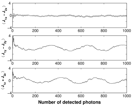
Figure 7: Evolution of $\langle J_{1x}-J_{2x}\rangle$, $\langle J_{1y}-J_{2y}\rangle$ and $\langle J_{1z}+J_{2z}\rangle$ corresponding to the simulation shown in Fig. 5(b).

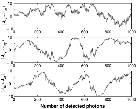
Figure 8: Evolution of $\langle J_{1x}-J_{2x}\rangle$, $\langle J_{1y}-J_{2y}\rangle$ and $\langle J_{1z}+J_{2z}\rangle$ corresponding to the simulation shown in Fig. 5(c).

VI Conclusion

We have presented a quantitative wave function analysis of the entanglement created by total population measurements on separate atomic samples by means of optical phase shifts. The analysis included wave function simulations where small samples were exposed to interaction with the optical fields in an interferometric set-up. We recall that more realistic experimental set-ups can be made , but they will be treated by the same formalism and lead to the same results. Our choice of parameters (only 20 atoms, high atom-field coupling) was not meant to correspond to a specific experiment, but it brings out results, that we may translate also to realistic experimental regimes. Note, however, that the present work should be extended to include also spontaneous emission by the atoms, if one wants to model experiments, where this has significant effects on the dynamics.

The entanglement protocol has already been implemented experimentally juls01 , and a theoretical analysis under an harmonic oscillator approximation has been presented. On one side our analysis supplements this existing analysis with a state vector perspective, and on the other hand it provides an analysis valid beyond the oscillator approximation, where in particular the emergence of a single maximally entangled state, and families of non-stationary states with different degrees of entanglement were identified. Since the experimentalist in principle knows the state vector conditioned on the outcome of the detection, it seems interesting to introduce feed-back thomsen02 , either by just resetting the system and start over again if an only weakly entangled state is prepared, or by suitably hitting the system during measurements.

References

- (1) A. Kuzmich, N. P. Bigelow and L. Mandel, Europhys. Lett. 42, 481 (1998).
- (2) K. Mølmer, Eur. Phys. J. D 5, 301 (1998).
- (3) I. Bouchoule and K. Mølmer, Preparation of spin squeezed atomic states by optical phase shift measurement, quant-ph/0205082, submitted to Phys. Rev. A.
- (4) A. Kuzmich and L. Mandel, Phys. Rev. A 60, 2346 (1999).
- (5) A. Kuzmich, L. Mandel, and N. P. Bigelow, Phys. Rev. Lett. 85, 1594 (2000).
- (6) L. -M. Duan, J.I. Cirac, P. Zoller, E. S. Polzik, Phys. Rev. Lett. 85, 5643 (2000).
- (7) B. Julsgaard, A. Kozhekin, and E. Polzik, Nature 413, 400 (2001).
- (8) Lu-Ming Duan, G. Giedke, J. I. Cirac, and P. Zoller, Phys. Rev. Lett. 84, 2722 (2000).
- (9) R. Simon, Phys. Rev. Lett. 84 2726 (2000).
- (10) C. H. Bennett, D. P. DiVincenzo, J. A. Smolin, and W. K. Wootters, Phys. Rev. A 54, 3824 (1996).
- (11) X. Wang and K. Mølmer, Eur. Phys. J. D. 18, 385-391 (2002).
- (12) L. K. Thomsen, S. Mancini, and H. M. Wiseman Phys. Rev. A 65, 061801 (2002).