A perturbative approach to non-Markovian stochastic Schrödinger equations

Abstract

In this paper we present a perturbative procedure that allows one to numerically solve diffusive non-Markovian Stochastic Schrödinger equations, for a wide range of memory functions. To illustrate this procedure numerical results are presented for a classically driven two level atom immersed in a environment with a simple memory function. It is observed that as the order of the perturbation is increased the numerical results for the ensembled average state $\rho_{\rm red}(t)$ approach the exact reduced state found via Imamoḡlu’s enlarged system method [Phys. Rev. A. 50, 3650 (1994)].

I Introduction

A common problem in physics is to model open quantum systems. They consists of a small system immersed in a bath (environment). Due to the large Hilbert space of the bath it is convenient to describe the system by its reduced state. The reduced state is defined as

$$\rho_{\rm red}(t)={\rm Tr}_{\rm bath}[|{\Psi(t)}\rangle\langle{\Psi(t)}|].$$ (1)

where $|{\Psi(t)}\rangle$ is the combined system state, found from the Schrödinger equation for the open quantum system.

It has been shown Nak58 ; Zwa60 by a projection-operator method that we can write a general master equation for the reduced state as

$$\dot{\rho}_{\rm red}(t)=-\frac{i}{\hbar}[\hat{H}(t),\rho_{\rm red}(t)]+\int_{0}^{t}{\cal K}(t,s)[\hat{L}]\rho_{\rm red}(s)ds$$ (2)

where ${\cal K}(t,s)[\hat{L}]$ is the ‘memory time’ superoperator. It (operators on) the system operator $\hat{L}$ and represents how the bath affects the system. The problem with this equation is that in general ${\cal K}(t,s)[\hat{L}]$ can not be explicitly evaluated.

The most notable approximation used is the Born-Markov one. This arises when the environmental influences on the system are instantaneous. Mathematical consistency requires that this results in a Lindblad master equation, of the form Lin76

$$\dot{\rho}_{\rm red}(t)=-\frac{i}{\hbar}[\hat{H}(t),\rho_{\rm red}(t)]+\gamma{\cal D}[\hat{L}]\rho_{\rm red}(t),$$ (3)

where ${\cal D}[\hat{L}]$ is the superoperator that represent the damping of the system into the bath. It has the form

$${\cal D}[\hat{L}]\rho_{\rm red}=\hat{L}\rho_{\rm red}\hat{L}^{\dagger}-\mbox{$\frac{1}{2}$}\hat{L}^{\dagger}\hat{L}\rho_{\rm red}-\mbox{$\frac{1}{2}$}\rho_{\rm red}\hat{L}^{\dagger}\hat{L}.$$ (4)

This equation can be solved deterministically GarZol00 or by the stochastic Schrödinger approach GarZol00 ; DalCasMol92 ; GarParZol92 ; Car93 .

For the non-Markovian situation there have been many attempts at finding solutions to Eq. (2). However, some have the problem that it is hard to ensure the positivity requirement on $\rho_{\rm red}(t)$ Red65 . A method that does ensure the positivity requirement on the reduced state is the non-Markovian stochastic Schrödinger equation (SSE) approach Dio96 ; DioStr97 ; DioGisStr98 ; StrDioGis99 ; Str01 ; Cre00 ; Bud00 ; GamWis02 . A non-Markovian SSE generates stochastic pure states ${|{\psi_{z}(t)}\rangle}$ that should satisfy

$$\rho_{\rm red}(t)=E[{|{\psi_{z}(t)}\rangle}{\langle{\psi_{z}(t)}|}],$$ (5)

where $z(t)$ is some noise function which is non-white and $E$ denotes the ensemble average over $z(t)$. To solve these non-Markovian SSE one has to take into account the past behavior of the system and bath, giving rise to a functional derivative in the attempt to derive a SSE. This presents a problem as for most systems an exact solution to the functional derivative does not exists. Thus at present an exact non-Markovian SSE only exists for simple systems, which can be solve exactly via other methods, like the undriven two level atom (TLA). For this and more examples see Ref. DioGisStr98 ; GamWis02 .

Recently Yu, Diósi, Gisin and Strunz (YDGS) have developed explicitly a ‘post-Markovian’ perturbation method to first order that allows solutions for systems that are close to the Markovian limit YuDioGisStr99 ; YuDioGisStr00 . In this paper we present a perturbation method that can be carried to arbitrary order and so is not limited to the post Markovian regime. However we must place a requirement on the form of the memory functions. This requirement is that the memory function must take the form

$$\alpha(t-s)=\sum_{j=1}^{J}|G_{j}|^{2}e^{-\kappa_{j}|t-s|/2-i(\omega_{j}-\Omega)(t-s)},$$ (6)

for some finite (and, in practice, relatively small) $J$. It should be noted also that we have not proven convergence of our perturbation theory and this theory is only valid for a zero-temperature bath.

The format of this paper is as follows. In Sec. II we present a general outline of the theory of non-Markovian SSE. This is basically a summary of the results of Refs. Dio96 ; DioStr97 ; DioGisStr98 ; StrDioGis99 ; GamWis02 . In Sec. III our perturbation method is presented. In Secs. IV we outline Imamo${\rm\bar{g}}$lu enlarged system method Ima94 ; SteIma96 . In Sec. V we apply our perturbation method to a simple system, a driven TLA and compare our results for $\rho_{\rm red}(t)$ with the enlarged system methods. In Sec. VI we investigate YDGS post-Markovian perturbation method YuDioGisStr99 ; YuDioGisStr00 . Finally we conclude with a discussion of the potential applications of our results in Sec. VII.

II Non-Markovian Stochastic Schrödinger Equations

In this section we will present an outline of the theory we presented in GamWis02 , which is an extension of Diósi, Gisin and Strunz (DGS) diffusive Non-Markovian SSEs Dio96 ; DioStr97 ; DioGisStr98 ; StrDioGis99 which allows for real-valued noise $z(t)$.

II.1 Underlying Dynamics

The non-Markovian SSEs developed in references GamWis02 ; Dio96 ; DioStr97 ; DioGisStr98 ; StrDioGis99 are valid when the dynamics of the open quantum system can be described by the total Hamiltonian

$$\hat{H}_{\rm tot}=\hat{H}_{\rm sys}\otimes\hat{1}+\hat{1}\otimes\hat{H}_{\rm bath}+\hat{V}.$$ (7)

The system Hamiltonian is $\hat{H}_{\rm sys}=\hat{H}_{\Omega}+\hat{H}$. The bath is modelled by a collection of harmonic oscillators, so the Hamiltonian for the bath is

$$\hat{H}_{\rm bath}=\hbar\sum_{k}\omega_{k}\hat{a}_{k}^{\dagger}\hat{a}_{k},$$ (8)

where $\hat{a}_{k}$ and $\omega_{k}$ are the lowering operator and angular frequency of the $k^{\rm th}$ mode respectively. This is the standard model for the electromagnetic field. The interaction Hamiltonian has the form

$$\hat{V}=i\hbar(\hat{L}\hat{b}^{\dagger}-\hat{L}^{\dagger}\hat{b}),$$ (9)

where we have defined the bath lowering operators $\hat{b}$ as $\hat{b}=\sum_{k}g_{k}\hat{a}_{k}$. That is, the coupling amplitude of the $k^{\rm th}$ mode to the system is $g_{k}$.

For calculation purposes we define the non-Markovian SSE in an interaction picture. This allows us to move the fast dynamics placed on the state by the Hamiltonians $\hat{H}_{\Omega}$ and $\hat{H}_{\rm bath}$ to the operators. The unitary evolution operator for this transformations is

$$U(t,0)=e^{-\frac{i}{\hbar}(\hat{H}_{\Omega}\otimes\hat{1}+\hat{1}\otimes\hat{H}_{\rm bath})(t-0)}.$$ (10)

Thus the combined state in the interaction picture is define as

$$|{\Psi(t)}\rangle=U^{\dagger}(t,0)|{\Psi(t)_{\rm Sch}}\rangle,$$ (11)

and an arbitrary operator $\hat{A}$ becomes

$$\hat{A}_{\rm int}=U^{\dagger}(t,0)\hat{A}U(t,0).$$ (12)

This allows us to write the Schrödinger equation as

$$d_{t}|{{\Psi}(t)}\rangle=-\frac{i}{\hbar}[\hat{H}_{\rm int}(t)+\hat{V}_{\rm int}(t)]|{\Psi(t)}\rangle,$$ (13)

where the Hamiltonians are

$$\hat{H}_{\rm int}(t) = U^{\dagger}(t,0)\hat{H}U(t,0),$$ (14)

and

$$\hat{V}_{\rm int}(t) = i\hbar[\hat{L}e^{-i\Omega t}\hat{b}_{\rm int}^{\dagger}(t)-\hat{L}^{\dagger}e^{i\Omega t}\hat{b}_{\rm int}(t)],$$ (15)

where

$$\hat{b}_{\rm int}(t) = \sum_{k}g_{k}\hat{a}_{k}e^{-i\omega_{k}t}.$$ (16)

Here we have finally restricted the form of $\hat{H}_{\Omega}$ to be such that $\hat{L}$ in the interaction picture simply rotates in the complex plane at frequency $\Omega$. That is $\hat{L}_{\rm int}(t)=\hat{L}e^{-i\Omega t}$.

II.2 Non-Markovian SSE-Defined

A non-Markovian SSE is a stochastic differential equation for the system state vector $|{\psi_{z}({t})}\rangle$ containing some non-white noise $z(t)$. It has the property that when $|{\psi_{z}({t})}\rangle\langle{\psi_{z}({t})}|$ is averaged over all possible $z(t)$ one obtains $\rho_{\rm red}$(t). It should be noted that for a single $\rho_{\rm red}(t)$, $z(t)$ can take many different functional forms, and we label these different forms as stochastic unravelings GamWis02 .

In Ref. GamWis02 we showed that non-Markovian SSEs can be derived from quantum measurement theory (QMT), where the different unravelings correspond to different measurements on the bath. The two unravelings we considered were the ‘coherent’ or ‘DGS’ Dio96 ; DioStr97 ; DioGisStr98 ; StrDioGis99 unraveling and the ‘quadrature’ unraveling. A special case of our quadrature unraveling was published in Ref. BasGhi02 .

As in the Markov limit we can define (at least) two non-Markovian SSEs, for each unraveling: one for $z(t)$ chosen from an ostensible distribution (a guessed distribution) and the other for its actual distribution. The former gives a non-Markovian SSE linear in the unnormalised state $|{\tilde{\psi}_{z}({t})}\rangle$, while the latter gives a non-Markovian SSE non-linear in the normalized state $|{\psi_{z}({t})}\rangle$. In Ref. GamWis02 we came to the conclusion that the solution of the actual non-Markovian SSE at time $t$ gives the state the system will be in if a measurement of the bath is performed at that time. Unlike in the Markov case, linking of the states through time to make a trajectory turns out to be a convenient fiction. However, it has been suggested that such trajectories can be given an interpretation within a non-standard QMT Lou01 ; BarLou02 .

II.2.1 Coherent Unravelling-Outlined

The first unravelling we consider is the ‘coherent’ unravelling. This unravelling arises when the bath is projected into a coherent state. We define the coherent state as

$$|{\{a_{k}\}}\rangle=\prod_{k}\frac{1}{\sqrt{\pi}\,}e^{-|a_{k}|^{2}/2}\sum_{n_{k}}\frac{a_{k}^{n_{k}}}{\sqrt{n_{k}!}\,}|{n_{k}}\rangle,$$ (17)

so that $\hat{1}=\prod_{k}\int|{a_{k}}\rangle\langle{a_{k}}|d^{2}a_{k}$.

In a measurement we can define an operator for the measurement process, the noise operator. For this measurement it must have the coherent basis as its eigenstate, so the noise operator is

$$\hat{z}(t)=\hat{b}_{\rm int}(t)e^{i\Omega t}=\sum_{k}g_{k}\hat{a}_{k}e^{-i\Omega_{k}t},$$ (18)

where $\Omega_{k}=\omega_{k}-\Omega$. The noise function (eigenvalue of the noise operator) is

$${z}(t)=\sum_{k}g_{k}{a}_{k}e^{-i\Omega_{k}t}.$$ (19)

where ${a}_{k}$ are the results of the projection in the coherent basis.

If we assume an ostensible distribution for ${a}_{k}$ as being the overlap of the coherent state with vacuum state, that is, it has the form

$${\Lambda}(\{a_{k}\})=\langle{\{0_{k}\}}|{\{a_{k}\}}\rangle\langle{\{a_{k}\}}|{\{0_{k}\}}\rangle={\pi^{-K}}{e^{-\sum_{k}|a_{k}|^{2}}},$$ (20)

where $K=\sum_{k}$. With this ostensible distribution the noise function has the following correlations

$$\tilde{E}[{z}(t)z^{*}(s)] = \alpha{(t-s)},$$ (21a)

$$\tilde{E}[{z}(t)z(s)] = 0.$$ (21b)

where the tilde above the $E$ refers to a average over the ostensible distribution. In Eq. (21a) we have defined $\alpha(t-s)$, this function we label the memory function. On a microscopic level it has the form

$$\alpha{(t-s)}=\sum_{k}|g_{k}|^{2}e^{-i\Omega_{k}(t-s)}.$$ (22)

Using the above ostensible distribution we can define a linear conditional system state as

$$|{\tilde{\psi}_{z}({t})}\rangle=\frac{\langle{\{a_{k}\}}|\Psi(t)\rangle}{\sqrt{{\Lambda}(\{a_{k}\})}\,}.$$ (23)

Taking the time derivative and using Eq. (13) we get a linear differential equation for $|{\tilde{\psi}_{z}({t})}\rangle$ of the from

$$\partial_{t}|{\tilde{\psi}_{z}({t})}\rangle = \Big{[}\frac{-i}{\hbar}\hat{H}_{\rm int}(t)+z^{*}(t)\hat{L}-\hat{L}^{\dagger}\int_{0}^{t}\alpha{(t-s)}$$ (24)

$$\times\frac{\delta}{\delta z^{*}(s)}ds\Big{]}|{\tilde{\psi}_{z}({t})}\rangle,$$

where ${\delta}/{\delta z^{*}(s)}$ represents a functional derivative. For a derivation of this equation see Ref. DioStr97 ; GamWis02 . The functional derivative in this equation stops us from calling this equation a non-Markovian SSE, as it means that $\partial_{t}|{\tilde{\psi}_{z}({t})}\rangle$ does not depend upon the state $|{\tilde{\psi}_{z}({t})}\rangle$ at all times for a single function $z(t)$, but rather also upon states for other noise functions. That is, we cannot stochastically choose $z(t)$ in order to generate a trajectory independent of other trajectories. Instead, all possible trajectories would have to be calculated in parallel, which in calculation terms amounts to solving the complete Schrödinger equation Eq. (13). However, as explained in Refs. GamWis02 ; DioGisStr98 ; StrDioGis99 if we can make the following ansatz

$$\frac{\delta}{\delta z^{*}(s)}|{\tilde{\psi}_{z}({t})}\rangle=~{}^{(0)}\hat{f}_{z}(t,s)|{\tilde{\psi}_{z}({t})}\rangle,$$ (25)

then we can write a linear non-Markovian SSE as

$$\partial_{t}|{\tilde{\psi}_{z}({t})}\rangle=\Big{[}\frac{-i}{\hbar}\hat{H}_{\rm int}(t)+z^{*}(t)\hat{L}-\hat{L}^{\dagger}~{}^{(0)}\hat{F}_{z}(t)\Big{]}|{\tilde{\psi}_{z}({t})}\rangle,$$ (26)

where the operator functional $~{}^{(0)}\hat{F}_{z}(t)$ is defined as

$$~{}^{(0)}\hat{F}_{z}(t)=\int_{0}^{t}\alpha(t-s)~{}^{(0)}\hat{f}_{z}(t,s)ds.$$ (27)

The significance of the superscripts $(0)$ proceeding these operators will become apparent in Sec. III.

To derive the actual (non-linear) non-Markovian SSE we need to condition the state on a noise function that is equivalent to the actual probability distribution,

$${P}(\{a_{k}\},t)=\langle{\Psi(t)}|{\{a_{k}\}}\rangle\langle{\{a_{k}\}}|{\Psi(t)}\rangle.$$ (28)

For most systems $|{\Psi(t)}\rangle$ is unknown. Nevertheless we can use a Girsanov transformation GamWis02 ; DioGisStr98 to relate the actual noise function to the ostensible noise function. In this case,

$$z(t)=z_{\Lambda}(t)+\int_{0}^{t}\alpha{(t-s)}\langle\hat{L}\rangle_{s}ds,$$ (29)

where $z_{\Lambda}(t)$ is equivalent to the noise function used in the ostensible case, satisfying the correlations defined in Eqs. (21a) and (21b). With the correct $z(t)$ the actual non-Markovian SSE for the normalised state is GamWis02 ; DioGisStr98

$$d_{t}|{\psi_{z}({t})}\rangle = \Big{[}{-\frac{i}{\hbar}\hat{H}_{\rm int}(t)}-(\hat{L}^{\dagger}-\langle\hat{L}^{\dagger}\rangle_{t})~{}^{(0)}\hat{F}_{z}(t)$$ (30)

$$+\Big{\langle}(\hat{L}^{\dagger}-\langle\hat{L}^{\dagger}\rangle_{t})~{}^{(0)}\hat{F}_{z}(t)\Big{\rangle}_{t}+z^{*}(t)$$

$$\times(\hat{L}-\langle\hat{L}\rangle_{t})\Big{]}|{\psi_{z}({t})}\rangle.$$

The notation $\langle\hat{L}\rangle_{t}$ is short hand for $\langle{\psi_{z}({t})}|\hat{L}|{\psi_{z}({t})}\rangle$. From Eq. (26) and Eq. (30) if the operator functional $~{}^{(0)}\hat{F}_{z}(t)$ is known for all time and for each noise function $z(t)$ we can solve the coherent non-Markovian SSE.

II.2.2 Quadrature Unravelling-Outlined

To obtain a non-Markovian SSE with real noise, it is natural to consider a quadrature noise operator,

$$\hat{z}(t)={\hat{b}_{\rm int}(t)e^{i\omega_{0}t}e^{-i\phi}+\hat{b}_{\rm int}^{\dagger}(t)e^{-i\omega_{0}t}e^{i\phi}},$$ (31)

where $\hat{b}_{\rm int}(t)$ is defined in equation (16) and $\phi$ is some arbitrary phase. The phase $\phi$ defines the measured quadrature: an $x$-quadrature measurement occurs when $\phi$ is set to zero, and the conjugate measurement of the $y$-quadrature occurs when $\phi=\pi/2$. Unless otherwise stated we will set $\phi$ to zero.

The measurement basis for the bath measurement is $|{\{q_{k}\}}\rangle$ and must satisfy

$$\hat{z}(t)|{\{q_{k}\}}\rangle=z(t)|{\{q_{k}\}}\rangle.$$ (32)

The problem with this noise function is that in general it is hard (maybe impossible) to work out a time-independent eigenstate in the interaction picture. However, we can find this eigenstate if we make the assumptions that for every mode $k$ there exists another mode, which we can label $-k$, such that $\Omega_{-k}=-\Omega_{k}$ and $g_{-k}=g^{*}_{k}$. These assumptions simply mean that the modes coupled to the system come in symmetric pairs about the frequency $\Omega$. Without loss of generality we can take the $g_{k}$’s to be real, absorbing any phases in the definitions of the bath operators. With all of these assumptions we can rewrite equation (31) as

$$\hat{z}(t)=\sum_{k>0}{2}g_{k}[\hat{X}_{k}^{+}\cos(\Omega_{k}t)+\hat{Y}_{k}^{-}\sin(\Omega_{k}t)].$$ (33)

Here we have introduced the two-mode quadrature operators

$$\hat{X}_{k}^{\pm} = (\hat{x}_{k}\pm\hat{x}_{-k})/{\sqrt{2}\,},$$ (34a)

$$\hat{Y}_{k}^{\pm} = (\hat{y}_{k}\pm\hat{y}_{-k})/{\sqrt{2}\,},$$ (34b)

where $\hat{x}_{k}$ and $\hat{y}_{k}$ are the quadratures of $\hat{a}_{k}$:

$$\hat{a}_{k}=({\hat{x}_{k}+i\hat{y}_{k}})/{\sqrt{2}\,}.$$ (35)

The measurement basis that satisfies Eq. (32), in the x-quadrature representation is

$$|{\{q_{k}\}}\rangle=\prod_{k>0}\int\frac{dx^{\prime}}{\sqrt{2\pi}\,}\Big{|}\frac{X_{k}^{+}-x^{\prime}}{\sqrt{2}\,}\Big{\rangle}_{-k}\Big{|}\frac{X_{k}^{+}+x^{\prime}}{\sqrt{2}\,}\Big{\rangle}_{k}e^{iY_{k}^{-}x^{\prime}}.$$ (36)

With this basis and the above noise operator the noise function for the quadrature measurement is

$$z(t)=\sum_{k>0}{2}g_{k}[X_{k}^{+}\cos(\Omega_{k}t)+Y_{k}^{-}\sin(\Omega_{k}t)],$$ (37)

which by definition is real.

Furthermore under the above assumptions the memory function $\alpha(t-s)$ in Eq. (22) reduces to

$$\beta{(t-s)}=2\sum_{k>0}|g_{k}|^{2}\cos[\Omega_{k}(t-s)].$$ (38)

As in the coherent case we define the ostensible distribution as the overlap between the vacuum state and $|{\{q_{k}\}}\rangle$, that is

$$\Lambda(\{X_{k},Y_{k}\})=\pi^{-K/2}{e^{-\sum_{k>0}({X_{k}^{+}}^{2}+{Y_{k}^{-}}^{2})}}.$$ (39)

With this distribution the correlation for the real-valued noise function is

$$\tilde{E}[z(t)z(s)]=\beta{(t-s)},$$ (40)

where the tilde, like before, means an average over the ostensible distribution. For this ostensible distribution the differential equation for $|{\tilde{\psi}_{z}({t})}\rangle$ is

$$\partial_{t}|{\tilde{\psi}_{z}({t})}\rangle = \Big{[}{-\frac{i}{\hbar}\hat{H}_{\rm int}(t)}+{z}(t)\hat{L}-\hat{L}_{x}\int_{0}^{t}\beta{(t-s)}$$ (41)

$$\times\frac{\delta}{\delta z(s)}ds\Big{]}|{\tilde{\psi}_{z}({t})}\rangle,$$

where $\hat{L}_{x}=\hat{L}+\hat{L}^{\dagger}$. Making the Ansatz,

$$\frac{\delta}{\delta z(s)}|{\tilde{\psi}_{z}({t})}\rangle=~{}^{(0)}\hat{q}_{z}(t,s)|{\tilde{\psi}_{z}({t})}\rangle,$$ (42)

the linear non-Markovian SSE is

$$\partial_{t}|{\tilde{\psi}_{z}({t})}\rangle=\Big{[}{-\frac{i}{\hbar}\hat{H}_{\rm int}(t)}+{z}(t)\hat{L}-\hat{L}_{x}~{}^{(0)}\hat{Q}_{z}(t)\Big{]}|{\tilde{\psi}_{z}({t})}\rangle,$$ (43)

where

$$~{}^{(0)}\hat{Q}_{z}(t)=\int_{0}^{t}\beta(t-s)~{}^{(0)}\hat{q}_{z}(t,s)ds.$$ (44)

To derive the actual non-Markovian SSE we need to calculate the correct noise function. The Girsanov transformation giving the actual real-valued $z(t)$ is GamWis02

$${z}(t) = z_{\Lambda}(t)+\int_{0}^{t}\langle\hat{L}_{x}\rangle_{s}\beta(t-s)ds,$$ (45)

where $z_{\Lambda}(t)$ satisfies the correlations defined in Eq. (40). The actual non-Markovian SSE for the quadrature unravelling is

$$d_{t}|{\psi_{z}({t})}\rangle = \Big{[}{-\frac{i}{\hbar}\hat{H}_{\rm int}(t)}-(\hat{L}_{x}-\langle\hat{L}_{x}\rangle_{t})~{}^{(0)}\hat{Q}_{z}(t)$$ (46)

$$+\Big{\langle}(\hat{L}_{x}-\langle\hat{L}_{x}\rangle_{t})~{}^{(0)}\hat{Q}_{z}(t)\Big{\rangle}_{t}+z(t)$$

$$\times(\hat{L}-\langle\hat{L}\rangle_{t})\Big{]}|{\psi_{z}({t})}\rangle.$$

Thus, if $~{}^{(0)}\hat{Q}_{z}(t)$ is known for $z(t)$ and all time then we can solve the quadrature non-Markovian SSE.

III Perturbation Method

To solve the non-Markovian SSE, and hence find $\rho_{\rm red}(t)$, for the coherent or quadrature unravelling we have to work out the operator functionals $~{}^{(0)}\hat{F}_{z}(t)$ and $~{}^{(0)}\hat{Q}_{z}(t)$ respectively. This has been done exactly only for systems for which an analytical solution for $\rho_{\rm red}(t)$ may be found by other means DioGisStr98 ; StrDioGis99 ; Cre00 or for systems with a small number of bath modes GamWis02 . In this section we to propose our perturbation technique for working out these functionals when exact solutions are not possible.

III.1 Perturbation Approach for the Coherent Unravelling

The perturbation that we are going to propose is only valid for memory functions of the form

$$\alpha(t-s)=\sum_{j=1}^{J}\alpha^{(j)}(t-s),$$ (47a)

where

$$\alpha^{(j)}(t-s)=|G_{j}|^{2}e^{-\kappa_{j}|t-s|/2}e^{-i\Omega_{j}(t-s)}.$$ (47b)

In principle this is always a valid decomposition for the memory function as in the $J\rightarrow\infty$ and $\kappa_{j}\rightarrow 0$ limit this memory function approaches the microscopic memory function displayed in Eq. (22). In Ref. SteIma96 the authors suggest that in practice most environments can be simulated with $J$ being quite small.

With this expansion for the memory function the functional $~{}^{(0)}\hat{F}_{z}(t)$ can be written as

$$~{}^{(0)}\hat{F}_{z}(t)=\sum_{j}~{}^{(0)}\hat{F}_{z}^{(j)}(t).$$ (48)

where

$$~{}^{(0)}\hat{F}_{z}^{(j)}(t)=\int_{0}^{t}\alpha^{(j)}(t-s)~{}^{(0)}\hat{f}_{z}(t,s)ds.$$ (49)

To calculate these operator functionals we set up a set of coupled nonlinear differential equations for $~{}^{(0)}\hat{F}_{z}^{(j)}(t)$. Taking the time derivative of Eq. (49) we get

$$\partial_{t}~{}^{(0)}\hat{F}_{z}^{(j)}(t) = \alpha^{(j)}(0)~{}^{(0)}\hat{f}_{z}(t,t)+\int_{0}^{t}[\partial_{t}\alpha^{(j)}(t-s)]$$ (50)

$$\times~{}^{(0)}\hat{f}_{z}(t,s)ds+\int_{0}^{t}\alpha^{(j)}(t-s)$$

$$\times\partial_{t}~{}^{(0)}\hat{f}_{z}(t,s)ds.\hskip 22.76228pt$$

The first term is easily evaluated using

$$^{(0)}\hat{f}_{z}(t,t)=\hat{L},$$ (51)

as derived in Appendix A. The second term is where our earlier decomposition of $\alpha(t-s)$ is used. We chose $\alpha^{(j)}(t-s)$ such that $\partial_{t}\alpha^{(j)}(t-s)\propto\alpha^{(j)}(t-s)$. This results in the second term equaling

$$-(\frac{\kappa_{j}}{2}+i\Omega_{j})~{}^{(0)}\hat{F}_{z}^{(j)}(t).$$ (52)

The third term involves the partial derivative $\partial_{t}[~{}^{(0)}\hat{f}_{z}(t,s)]$. To find this we use the fact that

$$\partial_{t}\frac{\delta}{\delta z^{*}(s)}|{\tilde{\psi}_{z}({t})}\rangle=\frac{\delta}{\delta z^{*}(s)}\partial_{t}|{\tilde{\psi}_{z}({t})}\rangle,$$ (53)

which is called the consistency condition in DioGisStr98 . This consistency condition is only valid for $t\neq s$ this is because at time $t=s$ the functional derivative is not well defined. Using Eq. (25) we can write the left-handed side (LHS) of the consistency condition as

$$\partial_{t}\frac{\delta}{\delta z^{*}(s)}|{\tilde{\psi}_{z}({t})}\rangle = [\partial_{t}~{}^{(0)}\hat{f}_{z}(t,s)]|{\tilde{\psi}_{z}({t})}\rangle$$ (54)

$$+~{}^{(0)}\hat{f}_{z}(t,s)\partial_{t}|{\tilde{\psi}_{z}({t})}\rangle.$$

Substituting Eq. (26) in for $\partial_{t}|{\tilde{\psi}_{z}({t})}\rangle$ gives

$$\partial_{t}\frac{\delta}{\delta z^{*}(s)}|{\tilde{\psi}_{z}({t})}\rangle = \Big{[}\partial_{t}~{}^{(0)}\hat{f}_{z}(t,s)-\frac{i}{\hbar}~{}^{(0)}\hat{f}_{z}(t,s)\hat{H}_{\rm int}(t)$$ (55)

$$+z^{*}(t)~{}^{(0)}\hat{f}_{z}(t,s)\hat{L}-~{}^{(0)}\hat{f}_{z}(t,s)$$

$$\times\hat{L}^{\dagger}~{}^{(0)}\hat{F}_{z}(t)\Big{]}|{\tilde{\psi}_{z}({t})}\rangle.$$

Using Eqs. (26) and (25) the right-handed side (RHS) of the consistency condition gives

$$\frac{\delta}{\delta z^{*}(s)}\partial_{t}|{\tilde{\psi}_{z}({t})}\rangle = \Big{[}-\frac{i}{\hbar}\hat{H}_{\rm int}(t)~{}^{(0)}\hat{f}_{z}(t,s)+z^{*}(t)\hat{L}$$ (56)

$$\times~{}^{(0)}\hat{f}_{z}(t,s)-\hat{L}^{\dagger}~{}^{(0)}\hat{F}_{z}(t)~{}^{(0)}\hat{f}_{z}(t,s)$$

$$-\hat{L}^{\dagger}\frac{\delta}{\delta z^{*}(s)}~{}^{(0)}\hat{F}_{z}(t)\Big{]}|{\tilde{\psi}_{z}({t})}\rangle.$$

Equating the LHS with the RHS gives

$$\partial_{t}~{}^{(0)}\hat{f}_{z}(t,s) = -\frac{i}{\hbar}[\hat{H}_{\rm int}(t),~{}^{(0)}\hat{f}_{z}(t,s)]+z^{*}(t)[\hat{L},$$ (57)

$$~{}^{(0)}\hat{f}_{z}(t,s)]-[\hat{L}^{\dagger}~{}^{(0)}\hat{F}_{z}(t),~{}^{(0)}\hat{f}_{z}(t,s)]$$

$$-\hat{L}^{\dagger}\frac{\delta}{\delta z^{*}(s)}~{}^{(0)}\hat{F}_{z}(t).$$

Substituting this equation with Eqs. (51) and (52) into Eq. (50) we get

$$\partial_{t}~{}^{(0)}\hat{F}^{(j)}_{z}(t) = |G_{j}|^{2}\hat{L}-(\frac{\kappa_{j}}{2}+i\Omega_{j})~{}^{(0)}\hat{F}^{(j)}_{z}(t)+z^{*}(t)$$

$$\times[\hat{L},~{}^{(0)}\hat{F}^{(j)}_{z}(t)]-\frac{i}{\hbar}[\hat{H}_{\rm int}(t),~{}^{(0)}\hat{F}^{(j)}_{z}(t)]$$

$$-[\hat{L}^{\dagger}~{}^{(0)}\hat{F}_{z}(t),~{}^{(0)}\hat{F}^{(j)}_{z}(t)]-\hat{L}^{\dagger}$$

$$\times\sum_{k}~{}^{(1)}\hat{F}_{z}^{(j,k)}(t),$$

where $~{}^{(1)}\hat{F}_{z}^{(j,k)}(t)$ is our first order functional. It has the form

$$~{}^{(1)}\hat{F}_{z}^{(j,k)}(t)=\int_{0}^{t}\alpha^{(j)}(t-s)~{}^{(1)}\hat{f}^{(k)}_{z}(t,s)ds,$$ (59)

where we have used the following Ansatz

$$\frac{\delta}{\delta z^{*}(s)}~{}^{(0)}\hat{F}^{(k)}_{z}(t)=~{}^{(1)}\hat{f}^{(k)}_{z}(t,s).$$ (60)

If we knew the form of $~{}^{(1)}\hat{F}_{z}^{(j,k)}(t)$ then Eq. (III.1) could be solved numerically.

To find the form of $~{}^{(1)}\hat{F}_{z}^{(j,k)}(t)$ we can take the time derivative of Eq. (59). Doing this we get

$$\partial_{t}~{}^{(1)}\hat{F}_{z}^{(j,k)}(t) = \alpha^{(j)}(0)~{}^{(1)}\hat{f}^{(k)}_{z}(t,t)+\int_{0}^{t}[\partial_{t}\alpha^{(j)}(t-s)]$$ (61)

$$\times~{}^{(1)}\hat{f}^{(k)}_{z}(t,s)ds+\int_{0}^{t}\alpha^{(j)}(t-s)$$

$$\times\partial_{t}~{}^{(1)}\hat{f}^{(k)}_{z}(t,s)ds.\hskip 14.22636pt$$

The first term is easy to work out. From Eq. (III.1) it follows that

$$~{}^{(1)}\hat{f}^{(k)}_{z}(t,t)=[\hat{L},~{}^{(0)}\hat{F}^{(k)}_{z}(t)].$$ (62)

The second term as before also simply evaluates to

$$-\Big{(}\frac{\kappa_{j}}{2}+i\Omega_{j}\Big{)}~{}^{(1)}\hat{F}^{(j,k)}_{z}(t).$$ (63)

The third term is worked out via a new consistency condition,

$$\partial_{t}\frac{\delta}{\delta z^{*}(s)}~{}^{(0)}\hat{F}^{(k)}_{z}(t)=\frac{\delta}{\delta z^{*}(s)}\partial_{t}~{}^{(0)}\hat{F}^{(k)}_{z}(t).$$ (64)

Substituting Eqs. (60) and (III.1) into this consistency condition gives

$$\partial_{t}~{}^{(1)}\hat{f}^{(k)}_{z}(t,s) = -(\frac{\kappa_{k}}{2}+i\Omega_{k})~{}^{(1)}\hat{f}_{z}^{(k)}(t,s)-\frac{i}{\hbar}[\hat{H}_{\rm int}(t),~{}^{(1)}\hat{f}^{(k)}_{z}(t,s)]+z^{*}(t)[\hat{L},~{}^{(1)}\hat{f}^{(k)}_{z}(t,s)]$$ (65)

$$-[\hat{L}^{\dagger}\sum_{l}~{}^{(1)}\hat{f}^{(l)}_{z}(t,s),~{}^{(0)}\hat{F}^{(k)}_{z}(t)]-[\hat{L}^{\dagger}\sum_{l}~{}^{(0)}\hat{F}^{(l)}_{z}(t),~{}^{(1)}\hat{f}^{(k)}_{z}(t,s)]$$

$$-\hat{L}^{\dagger}\sum_{l}\frac{\delta}{\delta z^{*}(s)}~{}^{(1)}\hat{F}_{z}^{(k,l)}(t).\hskip 14.22636pt$$

Substituting all these terms into Eq. (61) gives

$$\partial_{t}~{}^{(1)}\hat{F}_{z}^{(j,k)}(t) = |G_{j}|^{2}[\hat{L},~{}^{(0)}\hat{F}^{(k)}_{z}(t)]-\Big{(}\frac{\kappa_{j}}{2}+i\Omega_{j}\Big{)}~{}^{(1)}\hat{F}^{(j,k)}_{z}(t)-\Big{(}\frac{\kappa_{k}}{2}+i\Omega_{k}\Big{)}~{}^{(1)}\hat{F}_{z}^{(j,k)}(t)$$ (66)

$$-\frac{i}{\hbar}[\hat{H}_{\rm int}(t),~{}^{(1)}\hat{F}^{(j,k)}_{z}(t)]+z^{*}(t)[\hat{L},~{}^{(1)}\hat{F}^{(j,k)}_{z}(t)]-[\hat{L}^{\dagger}\sum_{l}~{}^{(1)}\hat{F}^{(j,l)}_{z}(t),~{}^{(0)}\hat{F}^{(k)}_{z}(t)]$$

$$-[\hat{L}^{\dagger}\sum_{l}~{}^{(0)}\hat{F}^{(l)}_{z}(t),~{}^{(1)}\hat{F}^{(j,k)}_{z}(t,s)]-\hat{L}^{\dagger}\sum_{l}~{}^{(2)}\hat{F}_{z}^{(j,k,l)}(t).$$

Where the last term is the second order functional, which equals

$$~{}^{(2)}\hat{F}_{z}^{(j,k,l)}(t)=\int_{0}^{t}\alpha^{(j)}(t-s)\frac{\delta}{\delta z^{*}(s)}~{}^{(1)}\hat{F}^{(k,l)}_{z}(t)ds.$$ (67)

Here we see that we can develop a general way for setting up an $n^{\rm th}$ order differential equations. The $n^{\rm th}$ order functional is

$$~{}^{(n)}\hat{F}_{z}^{(j,k,...,l)}(t)=\int_{0}^{t}\alpha^{(j)}(t-s)~{}^{(n)}\hat{f}^{(k,...,l)}_{z}(t,s)ds,$$ (68)

where we have used the Ansatz

$$\frac{\delta}{\delta z^{*}(s)}~{}^{(n-1)}\hat{F}^{(k,...,l)}_{z}(t)=~{}^{(n)}\hat{f}^{(k,...,l)}_{z}(t,s).$$ (69)

The differential equation for the $n^{\rm th}$ order functional is

$$\partial_{t}~{}^{(n)}\hat{F}_{z}^{(j,k,...,l)}(t) = \alpha^{(j)}(0)~{}^{(n)}\hat{f}^{(k,...,l)}_{z}(t,t)$$

$$+\int_{0}^{t}[\partial_{t}\alpha^{(j)}(t-s)]~{}^{(n)}\hat{f}^{(k,...,l)}_{z}(t,s)ds$$

$$+\int_{0}^{t}\alpha^{(j)}(t-s)\partial_{t}~{}^{(n)}\hat{f}^{(k,...,l)}_{z}(t,s)ds.$$

The first term can always be calculated by the $(n-1)^{\rm th}$ differential equation. The second term is always simple to calculate as $\partial_{t}\alpha^{(j)}(t-s)\propto\alpha^{(j)}(t-s)$ and the third term is always calculable by the $(n-1)^{\rm th}$ order consistency condition

$$\partial_{t}\frac{\delta}{\delta z^{*}(s)}~{}^{(n-1)}\hat{F}^{(k,...,l)}_{z}(t)=\frac{\delta}{\delta z^{*}(s)}\partial_{t}~{}^{(n-1)}\hat{F}^{(k,...,l)}_{z}(t).$$ (71)

The $n^{\rm th}$ order perturbation method propose is to terminate this series by setting $~{}^{(n)}\hat{F}_{z}^{(j,k,...,l)}(t)$ equal to an arbitrary operator. The simplest scheme would be to set this operator to zero, but to keep the theory consistent with the Markov limit for all orders, we set $~{}^{(n)}\hat{F}_{z}^{(j,k,...,l)}(t)$ in the following manner. The zeroth order perturbation aries when we use the approximation

$$~{}^{(0)}\hat{F}_{z}^{(j)}(t)\simeq\int_{0}^{t}\alpha^{(j)}(t-s)ds\frac{\delta}{\delta z^{*}(t)}=\int_{0}^{t}\alpha^{(j)}(t-s)ds\hat{L}.$$ (72)

Note that the approximation here is the replacement of $\delta/\delta z^{*}(s)$ by $\delta/\delta z^{*}(t)$. The first order perturbation arises when we use the approximation

$$~{}^{(1)}\hat{F}_{z}^{(j,k)}(t) \simeq \int_{0}^{t}\alpha^{(j)}(t-s)ds\frac{\delta~{}^{(0)}\hat{F}^{(k)}_{z}(t)}{\delta z^{*}(t)}$$ (73)

$$= \int_{0}^{t}\alpha^{(j)}(t-s)ds[\hat{L},~{}^{(0)}\hat{F}^{(k)}_{z}(t)]$$

and $~{}^{(0)}\hat{F}_{z}^{(j)}(t)$ is calculated via Eq. (III.1). The $n^{\rm th}$ order perturbation arises when we use the approximation

$$~{}^{(n)}\hat{F}_{z}^{(j,k,...,l)}(t) \simeq \int_{0}^{t}\alpha^{(j)}(t-s)ds\frac{\delta~{}^{(n-1)}\hat{F}^{(k,...,l)}_{z}(t)}{\delta z^{*}(t)}$$

$$= \int_{0}^{t}\alpha^{(j)}(t-s)ds[\hat{L},~{}^{(n-1)}\hat{F}^{(k,...,l)}_{z}(t)]$$

and $~{}^{(0)}\hat{F}_{z}^{(j)}(t),...,~{}^{(n-1)}\hat{F}_{z}^{(j,...,k)}(t)$ are calculated via Eqs. (III.1), (66) and (III.1). The physical motivations for choosing this type of expansion are;
     a) For most system the memory function will decay and thus the most dominant term in the functional derivative will be the value as $s\rightarrow t$.
    b) Only $~{}^{(0)}\hat{F}^{(j)}_{z}(t)$ affects the system directly, so the further removed the approximation the more accurate we expect the approximation to be.
    c) In the Markovian limit, only the zero order term is needed.

To summarize this perturbation method, for environments which can be modelled by Eq. (47), it is possible to obtain a perturbative solution for the coherent non-Markovian SSE. From these SSEs it is possible to generate a perturbative solution for $\rho_{\rm red}(t)$, which by definition will always be positive. The number of coupled complex differential equations that are required for this technique is

$$d^{2}(J^{n}+J^{n-1}+...+J)+d+J=d^{2}J\frac{J^{n}-1}{J-1}+d+J$$ (75)

where $d$ is the system dimension, $J$ is the number of exponentials required to simulate the memory function and $n$ is the order of the perturbation. The first term represents the number of equations needed to simulate the functional derivative. The next term $d$ is for the $d$ complex amplitudes of the system. The final term $J$ is for the stochastic equations needed to generate the noise function $z(t)$.

III.2 Perturbation Approach for the Quadrature Unravelling

The perturbation method in the quadrature case is essentiality the same as the coherent case, but the memory function expressed in Eq. (47b) is too general. This is because the memory function for the quadrature unraveling must be consistent with the assumptions stated below Eq. (32). The most general memory function that satisfies these requirements is

$$\beta(t-s)=\sum_{j}^{{}^{\prime}}\beta^{(j,\cos)}(t-s),$$ (76a)

where

$$\beta^{(j,\cos)}(t-s)=2|G_{j}|^{2}e^{-\kappa_{j}|t-s|/2}\cos[\Omega_{j}(t-s)].$$ (76b)

This presents a problem as $\partial_{t}\beta^{(j,\cos)}(t-s)$ is not proportional to $\beta^{(j,\cos)}(t-s)$. To get around this we define a new function $\beta^{(j,\sin)}(t-s)$ as

$$\beta^{(j,\sin)}(t-s)=2|G_{j}|^{2}e^{-\kappa_{j}|t-s|/2}\sin(\Omega_{j}(t-s)),$$ (77)

and two functionals

$$~{}^{(0)}\hat{Q}_{z}^{(j,\cos)}(t) = \int_{0}^{t}\beta^{(j,\cos)}(t-s)\hat{q}_{z}(t,s)ds,$$ (78a)

$$~{}^{(0)}\hat{Q}_{z}^{(j,\sin)}(t) = \int_{0}^{t}\beta^{(j,\sin)}(t-s)\hat{q}_{z}(t,s)ds.$$ (78b)

The functional $~{}^{(0)}\hat{Q}_{z}(t)$ is the found by

$$~{}^{(0)}\hat{Q}_{z}(t)=\sum_{j}~{}^{(0)}\hat{Q}_{z}^{(j,\cos)}(t).$$ (79)

Taking the time derivative of Eqs. (78a) and (78b) we get

$$d_{t}~{}^{(0)}\hat{Q}^{(j,\cos)}_{z}(t) = \beta^{(j,\cos)}(t,t)~{}^{(0)}\hat{q}_{z}(t,t)$$

$$+\int_{0}^{t}[\partial_{t}\beta^{(j,\cos)}(t-s)]~{}^{(0)}\hat{q}_{z}(t,s)ds$$

$$+\int_{0}^{t}\beta^{(j,\cos)}(t-s)\partial_{t}~{}^{(0)}\hat{q}_{z}(t,s)ds,$$

$$d_{t}~{}^{(0)}\hat{Q}^{(j,\sin)}_{z}(t) = \int_{0}^{t}[\partial_{t}\beta^{(j,\sin)}(t-s)]~{}^{(0)}\hat{q}_{z}(t,s)ds$$

$$+\int_{0}^{t}\beta^{(j,\sin)}(t-s)\partial_{t}~{}^{(0)}\hat{q}_{z}(t,s)ds.$$

As in the coherent case it can be shown that $~{}^{(0)}\hat{q}_{z}(t,t)=\hat{L}$. The two terms involving the derivative of $\beta^{(j,\cos)}(t-s)$ and $\beta^{(j,\sin)}(t-s)$ by definition give

$$\int_{0}^{t}\partial_{t}\beta^{(j,\cos)}(t-s)~{}^{(0)}\hat{q}_{z}(t,s)ds = -\frac{\kappa_{j}}{2}~{}^{(0)}\hat{Q}^{(j,\cos)}_{z}(t)$$ (81a)

$$-\Omega_{j}~{}^{(0)}\hat{Q}^{(j,\sin)}_{z}(t)$$

$$\int_{0}^{t}\partial_{t}\beta^{(j,\sin)}(t-s)~{}^{(0)}\hat{q}_{z}(t,s)ds = -\frac{\kappa_{j}}{2}~{}^{(0)}\hat{Q}^{(j,\sin)}_{z}(t)$$ (81b)

$$+\Omega_{j}~{}^{(0)}\hat{Q}^{(j,\cos)}_{z}(t).\hskip 22.76228pt$$

The last two terms require finding $\partial_{t}~{}^{(0)}\hat{q}_{z}(t,s)$. As in the coherent case this is found by the consistency condition

$$\partial_{t}\frac{\delta}{\delta z(s)}|{\tilde{\psi}_{z}({t})}\rangle=\frac{\delta}{\delta z(s)}\partial_{t}|{\tilde{\psi}_{z}({t})}\rangle,$$ (82)

yielding

$$\partial_{t}~{}^{(0)}\hat{q}_{z}(t,s) = -\frac{i}{\hbar}[\hat{H}_{\rm int}(t),~{}^{(0)}\hat{q}_{z}(t,s)]+z(t)[\hat{L},$$ (83)

$$~{}^{(0)}\hat{q}_{z}(t,s)]-[\hat{L}_{x}~{}^{(0)}\hat{Q}_{z}(t),~{}^{(0)}\hat{q}_{z}(t,s)]$$

$$-\hat{L}_{x}\frac{\delta}{\delta z(s)}~{}^{(0)}\hat{Q}_{z}(t).$$

Substituting these terms into Eq. (80) we get

$$d_{t}~{}^{(0)}\hat{Q}^{(j,\cos)}_{z}(t) = 2|G_{j}|^{2}\hat{L}-\frac{\kappa_{j}}{2}~{}^{(0)}\hat{Q}^{(j,\cos)}_{z}(t)-\Omega_{j}~{}^{(0)}\hat{Q}^{(j,\sin)}_{z}(t)-\frac{i}{\hbar}[\hat{H}_{\rm int}(t),~{}^{(0)}\hat{Q}^{(j,\cos)}_{z}(t)]$$ (84a)

$$+z(t)[\hat{L},~{}^{(0)}\hat{Q}^{(j,\cos)}_{z}(t)]-[\hat{L}_{x}~{}^{(0)}\hat{Q}_{z}(t),~{}^{(0)}\hat{Q}^{(j,\cos)}_{z}(t)]$$

$$-\hat{L}_{x}\sum_{k}~{}^{(1)}\hat{Q}^{(j,k,\cos,\cos)}_{z}(t),$$

$$d_{t}~{}^{(0)}\hat{Q}^{(j,\sin)}_{z}(t) = -\frac{\kappa_{j}}{2}~{}^{(0)}\hat{Q}^{(j,\sin)}_{z}(t)+\Omega_{j}~{}^{(0)}\hat{Q}^{(j,\cos)}_{z}(t)-\frac{i}{\hbar}[\hat{H}_{\rm int}(t),~{}^{(0)}\hat{Q}^{(j,\sin)}_{z}(t)]+z(t)[\hat{L},~{}^{(0)}\hat{Q}^{(j,\sin)}_{z}(t)]$$ (84b)

$$-[\hat{L}_{x}~{}^{(0)}\hat{Q}_{z}(t),^{(0)}~{}^{(0)}\hat{Q}^{(j,\sin)}_{z}(t)]-\hat{L}_{x}\sum_{k}~{}~{}^{(1)}\hat{Q}^{(j,k,\sin,\cos)}_{z}(t),$$

where

$$~{}^{(1)}\hat{Q}^{(j,k,\cos,\cos)}_{z}(t)=\int_{0}^{t}\beta^{(j,\cos)}(t,s)\frac{\delta~{}^{(0)}\hat{Q}^{(k,\cos)}_{z}(t)}{\delta z(s)}ds,$$ (85a)

$$~{}^{(1)}\hat{Q}^{(j,k,\sin,\cos)}_{z}(t)=\int_{0}^{t}\beta^{(j,\sin)}(t,s)\frac{\delta~{}^{(0)}\hat{Q}^{(k,\cos)}_{z}(t)}{\delta z(s)}ds.$$ (85b)

The higher order functional differential equations are found in the same manner as in the coherent case, except the form of $\beta(t-s)$ results in $2^{n}$ as many equations for order $n$.

The perturbation expansion is similar for this unravelling, the only difference being that we have $2^{n}$ operators to approximate. The $0^{\rm th}$ order approximation is to set the $0^{\rm th}$ order functionals to

$$~{}^{(0)}\hat{Q}^{(j,\cos)}_{z}(t) = \int_{0}^{t}\beta^{(j,\cos)}(t,s)ds\hat{L}$$ (86a)

$$~{}^{(0)}\hat{Q}^{(j,\sin)}_{z}(t) = \int_{0}^{t}\beta^{(j,\sin)}(t,s)ds\hat{L}.$$ (86b)

The first order approximation is to set the four first order functionals to

$$~{}^{(1)}\hat{Q}^{(j,k,\cos,\cos)}_{z}(t) = \int_{0}^{t}\beta^{(j,\cos)}(t,s)ds[\hat{L},~{}^{(0)}\hat{Q}^{(k,\cos)}_{z}(t)],$$

$$~{}^{(1)}\hat{Q}^{(j,k,\sin,\cos)}_{z}(t) = \int_{0}^{t}\beta^{(j,\sin)}(t,s)ds[\hat{L},~{}^{(0)}\hat{Q}^{(k,\cos)}_{z}(t)],$$

$$~{}^{(1)}\hat{Q}^{(j,k,\cos,\sin)}_{z}(t) = \int_{0}^{t}\beta^{(j,\cos)}(t,s)ds[\hat{L},~{}^{(0)}\hat{Q}^{(k,\sin)}_{z}(t)],$$

$$~{}^{(1)}\hat{Q}^{(j,k,\sin,\sin)}_{z}(t) = \int_{0}^{t}\beta^{(j,\sin)}(t,s)ds[\hat{L},~{}^{(0)}\hat{Q}^{(k,\sin)}_{z}(t)].$$

and we calculate the ${0^{\rm th}}$ order functionals via Eq. (84).

IV Enlarged System Approach

To test the accuracy of our perturbation method we compare our results for the reduced state with the reduced state found via the enlarged system method of Imamo$\bar{\rm g}$lu Ima94 ; SteIma96 . An example of how this method is applied to a non-Markovian system can be found in Ref. CaoLonWeiCao01 .

For those who are not familiar with the enlarged system method, we provide a short proof that the reduced system dynamics are exactly reproduced by the enlarged system method provided that $\alpha(t-s)$, called $\Gamma(\tau)$ in Refs Ima94 ; SteIma96 , is of the form

$$\alpha(t-s)=\sum_{j}|G_{j}|^{2}e^{-\kappa_{j}|t-s|/2-i\Omega_{j}(t-s)},$$ (88)

which is the same as Eq. (47).

The total Hamiltonian for the enlarged system is

$$\hat{H}_{\rm tot} = \hat{H}_{\rm sys}+\hbar\sum_{j}\omega_{j}\hat{c}_{j}^{\dagger}\hat{c}_{j}+\hbar\sum_{j}\int_{-\infty}^{\infty}d\omega$$

$$\times\omega\hat{\nu}_{j}(\omega)^{\dagger}\hat{\nu}_{j}(\omega)+i\hbar\sum_{j}[G^{*}_{j}\hat{L}\hat{c}_{j}^{\dagger}-G_{j}\hat{L}^{\dagger}\hat{c}_{j}]$$

$$+i\hbar\sum_{j}\int_{-\infty}^{\infty}d\omega\sqrt{\frac{\kappa_{j}}{2\pi}}\,[\hat{\nu}^{\dagger}_{j}(\omega)\hat{c}_{j}-\hat{\nu}_{j}(\omega)\hat{c}_{j}^{\dagger}],$$

where $\hat{H}_{\rm sys}=\hat{H}_{\Omega}+\hat{H}$, $\hat{c}_{j}$ is the annihilation operator for the $j^{\rm th}$ added oscillator and $\hat{\nu}_{j}(\omega)$ is the Markovian bath operator with the correlation

$$[\hat{\nu}_{j}(\omega),\hat{\nu}_{k}^{\dagger}(\omega)]=\delta_{j,k}\delta(\omega-\omega^{\prime}).$$ (90)

If this is to be the same as Eq. (7), then the first two lines of Eq. (IV) must give $\hat{H}_{\rm sys}+\hat{H}_{\rm bath}$ and the final line $\hat{V}$. Going to the same interaction picture as we did in Sec. II.1, that is with respect to the Hamiltonians $\hat{H}_{\Omega}$ and $\hat{H}_{\rm bath}$, we get

$$\hat{V}_{\rm int}(t)=i\hbar\sum_{j}[G^{*}_{j}\hat{L}e^{-i\Omega t}\hat{c}_{j}(t)^{\dagger}-G_{j}\hat{L}^{\dagger}e^{i\Omega t}\hat{c}_{j}(t)].$$ (91)

Comparing with Eq. (15), for the enlarged system method to be correct we need $\hat{b}_{\rm int}(t)=\sum_{j}G_{j}\hat{c}_{j}(t)$. To calculate $\hat{c}_{j}(t)$ we use the fact that

$$d_{t}\hat{c}_{j}(t)=-i\omega_{j}\hat{c}_{j}(t)-\frac{\kappa_{j}}{2}\hat{c}_{j}(t)-\sqrt{\kappa_{j}}\,\hat{\nu}_{{\rm in},j}(t)$$ (92)

where $\hat{\nu}_{{\rm in},j}(t)$ is the input field which has a time commutator $[\hat{\nu}_{{\rm in},j}(t),\hat{\nu}^{\dagger}_{{\rm in},k}(s)]=\delta_{j,k}\delta(t-s)$. For a derivation of equation Eq. (92) see Ref. GarCol85 . This can be integrated to give

$$\hat{c}_{j}(t) = \sqrt{\kappa_{j}}\,\int_{0}^{t}e^{-\kappa_{j}(t-s)/2-i\omega_{j}(t-s)}\hat{\nu}_{{\rm in},j}(s)ds$$ (93)

$$+\hat{c}_{j}(0)e^{-\kappa_{j}t/2-i\omega_{j}t}.$$

It not obvious that $\sum_{j}G_{j}\hat{c}_{j}(t)$ is the same as Eq. (16). However the time commutator for the bath operators is

$$[\hat{b}_{\rm int}(t),\hat{b}^{\dagger}_{\rm int}(s)]e^{i\Omega(t-s)}=\alpha(t-s).$$ (94)

In terms of the enlarged system this means

$$\sum_{j,k}G_{j}G^{*}_{k}[\hat{c}_{j}(t),\hat{c}^{\dagger}_{k}(s)]e^{i\Omega(t-s)}$$

$$=\sum_{j}|G_{j}|^{2}e^{-\kappa_{j}(t+s)/2-i(\omega_{j}-\Omega)(t-s)}[1$$

$$+{\kappa_{j}}\int_{0}^{t}\int_{0}^{s}e^{+\kappa_{j}(t^{\prime}+s^{\prime})/2+i\omega_{j}(t^{\prime}-s^{\prime})}\delta(t^{\prime}-s^{\prime})dt^{\prime}ds^{\prime}]$$

$$=\sum_{j}|G_{j}|^{2}e^{-\kappa_{j}|t-s|/2-i(\omega_{j}-\Omega)(t-s)}$$

$$=\alpha(t-s),$$ (95)

provide $\alpha(t-s)$ has the form depicted in Eq. (88). It should noted that this result is exact. It is not necessary to discard initial transients as in the derivation in Ref SteIma96 .

Since we have shown that the total Hamiltonian for the enlarged system is equivalent to the standard non-Markovian, then the total states $|{\Psi_{Sch}(t)}\rangle$ must be the same. We can define a reduced state (in the Schrödinger picture) for the enlarged system as $W_{\rm Sch}(t)$ which has the Markovian master equation

$$d_{t}W_{\rm Sch}(t) = -\frac{i}{\hbar}[\hat{H}_{\Omega}+\hat{H}+\hbar\sum_{j}\omega_{j}\hat{c}_{j}^{\dagger}\hat{c}_{j}+i\hbar\sum_{j}$$ (96)

$$\times(G^{*}_{j}\hat{L}\hat{c}_{j}^{\dagger}-G_{j}\hat{L}^{\dagger}\hat{c}_{j}),W_{\rm Sch}(t)]$$

$$+\sum_{j}\kappa_{j}{\cal D}[\hat{c}_{j}]W_{\rm Sch}(t).$$

The reduced state for the system in the $\Omega$-interaction picture is

$$\rho_{\rm red}(t)=e^{\frac{i}{\hbar}\hat{H}_{\Omega}t}Tr_{\rm enl}[W_{\rm Sch}(t)]e^{-\frac{i}{\hbar}\hat{H}_{\Omega}t}=Tr_{\rm enl}[W_{\rm red}(t)],$$ (97)

where the trace is performed over the added oscillators and

$$W_{\rm red}(t)=e^{{i}\sum_{j}\omega_{j}\hat{c}_{j}^{\dagger}\hat{c}_{j}t+\frac{i}{\hbar}\hat{H}_{\Omega}t}W_{\rm Sch}(t)e^{-{i}\sum_{j}\omega_{j}\hat{c}_{j}^{\dagger}\hat{c}_{j}t-\frac{i}{\hbar}\hat{H}_{\Omega}t}.$$ (98)

This allows us to define a new master equation for the reduced state $W_{\rm red}(t)$ as

$$d_{t}W_{\rm red}(t) = [-\frac{i}{\hbar}\hat{H}_{\rm int}+\sum_{j}[G^{*}_{j}\hat{L}\hat{c}_{j}^{\dagger}e^{i(\omega_{j}-\Omega)t}$$

$$-G_{j}\hat{L}^{\dagger}\hat{c}_{j}e^{-i(\omega_{j}-\Omega)t}],W_{\rm red}(t)]$$

$$+\sum_{j}\kappa_{j}{\cal D}[\hat{c}_{j}]W_{\rm red}(t).$$

which can be solved by standard Markovian techniques, for example quantum trajectories DalCasMol92 ; GarParZol92 ; Car93 .

V Numerical Example: The Driven Two Level Atom

In this section we apply our theory to a driven TLA with a simple non-Markovian memory function.

$$\alpha(t-s)=\frac{\gamma\kappa}{4}e^{i(\omega_{\rm env}-\Omega)(t-s)}e^{-\kappa|t-s|/2},$$ (100)

where $\omega_{\rm env}$ is the central frequency of the environment, $\kappa$ represent the exponential decay of bath memory and $\gamma$ is the Markovian limit decay rate. That is, in the $\kappa\rightarrow\infty$ limit, $\alpha(t-s)=\gamma\delta(t-s)$, which is the Markovian limit of the memory function GamWis02 . We choose an interaction picture such the $\Omega=\omega_{\rm env}$ so that this memory function is simplifies to

$$\alpha(t-s)=\frac{\gamma\kappa}{4}e^{-\kappa|t-s|/2},$$ (101)

which is consistent with the quadrature unravelings assumptions. This results in $\alpha(t-s)=\beta(t-s)$. However before we apply our theory to the TLA let us revise the standard TLA model.

V.1 The TLA

The TLA is one of the most simple quantum systems to envisage. It consists of two levels, an excited state $|{e}\rangle$ of energy $\hbar\omega_{e}$ and a ground state $|{g}\rangle$ of energy $\hbar\omega_{g}$. We define the difference in these energies as $\hbar\omega_{0}$ and the zero point energy is taken to be the mid point energy $\hbar(\omega_{e}+\omega_{g})/2=0$. This allows us to define a system Hamiltonian as

$$\hat{H}_{\rm sys}=\hbar\frac{\omega_{0}}{2}\hat{\sigma}_{z}$$ (102)

where $\hat{\sigma}_{z}=|{e}\rangle\langle{e}|-|{g}\rangle\langle{g}|$ is one of the spin matrices for the TLA.

Since we are dealing with open quantum systems we consider the dynamics of the TLA immersed in the electromagnetic field (the bath). In the Schrödinger picture with the dipole and rotating wave approximation (RWA) approximation the interaction Hamiltonian is

$$\hat{V}=i\hbar\sum_{k}(g^{*}_{k}\hat{\sigma}\hat{a}_{k}^{\dagger}-g_{k}\hat{\sigma}^{\dagger}\hat{a}_{k}),$$ (103)

where $\hat{\sigma}$ is the lowering operator for the TLA. This is the same form as Eq. (9) with $\hat{L}=\hat{\sigma}$, so the above non-Markovian SSE theory is applicable to this system.

If we have a TLA driven by a classical electromagnetic field the system Hamiltonian for the TLA under the RWA approximation is

$$\hat{H}_{\rm sys}=\hbar\frac{\omega_{0}}{2}\hat{\sigma}_{z}+\hbar\frac{\chi}{2}[\hat{\sigma}e^{i\omega_{\rm dr}t}+\hat{\sigma}^{\dagger}e^{-i\omega_{\rm dr}t}],$$ (104)

where $\chi$ is the Rabi frequency and $\omega_{\rm dr}$ is the driving frequency of the classical field. However as shown in Eq. (7) we can also write $\hat{H}_{\rm sys}$ as $\hat{H}_{\Omega}+\hat{H}(t)$. If $\hat{H}_{\Omega}={\Omega}\hat{\sigma}_{z}/{2}$, then in the $\Omega$ interaction picture gives

$$\hat{H}_{\rm int}(t)=\hbar\frac{\omega_{0}-\Omega}{2}\hat{\sigma}_{z}+\hbar\frac{\chi}{2}[\hat{\sigma}e^{i(\omega_{\rm dr}t-\Omega t)}+\hat{\sigma}^{\dagger}e^{-i(\omega_{\rm dr}t-\Omega t)}],$$ (105)

For our purposes we assume $\Omega=\omega_{\rm dr}$. So

$$\hat{H}_{\rm int}(t)=\hbar\frac{\Delta}{2}\hat{\sigma}_{z}+\hbar\frac{\chi}{2}\hat{\sigma}_{x},$$ (106)

where $\Delta=\omega_{0}-\Omega$ is the detuning.

For the TLA the reduced state can be written in terms of the real Bloch vector components $x(t)$, $y(t)$, $z(t)$ as

$$\rho_{\rm red}(t)=\mbox{$\frac{1}{2}$}[\hat{I}+x(t)\hat{\sigma}_{x}+y(t)\hat{\sigma}_{y}+z(t)\hat{\sigma}_{z}].$$ (107)

V.2 Enlarged System Method

For the driven TLA with a memory function given by Eq. (100) the master equation for the enlarged systems is

$$d_{t}W_{\rm red}(t) = [-\frac{i\Delta}{2}\hat{\sigma}_{z}-\frac{i\chi}{2}\hat{\sigma}_{x}+\frac{\gamma\kappa}{4}(\hat{\sigma}\hat{c}-\hat{\sigma}^{\dagger}\hat{c}),$$ (108)

$$W_{\rm red}(t)]+\kappa{\cal D}[\hat{c}]W_{\rm red}(t).$$

Using $\gamma=1$, $\kappa=1$, $\chi=5$ and $\Delta=3$ the reduced state is shown in Fig. 1. For this simple case it was noted that the truncation error involved in the enlarged system state method was negligible. Because of this we use this reduced state for comparison with the ensemble average of the non-Markovian SSEs.

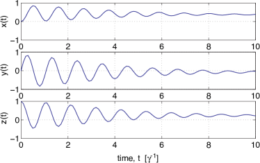
Figure 1: This figure depicts the Bloch vector components of the reduced state of a driven TLA calculated by the enlarged system method. In this figure all calculations were done using the initial system state $|{\psi(0)}\rangle=|{e}\rangle$ with system parameters $\gamma=1$, $\kappa=1$, $\chi=5$ and $\Delta=3$. Time is measured in units $\gamma^{-1}$.

V.3 Coherent Unravelling-TLA

Applying the coherent non-Markovian SSE theory to the driven TLA, we find that we can rewrite the actual non-Markovian SSE as

$$d_{t}|{\psi_{z}({t})}\rangle = \Big{[}-i\frac{\Delta}{2}\hat{\sigma}_{z}-i\frac{\chi}{2}\hat{\sigma}_{x}-(\hat{\sigma}^{\dagger}-\langle\hat{\sigma}^{\dagger}\rangle_{t})$$ (109)

$$\times~{}^{(0)}\hat{F}_{z}(t)+\Big{\langle}(\hat{\sigma}^{\dagger}-\langle\hat{\sigma}^{\dagger}\rangle_{t})~{}^{(0)}\hat{F}_{z}(t)\Big{\rangle}_{t}$$

$$+z^{*}(t)(\hat{\sigma}-\langle\hat{\sigma}\rangle_{t})\Big{]}|{\psi_{z}({t})}\rangle,$$

and the noise function for the TLA becomes

$$z(t)=z_{\Lambda}(t)+\int_{0}^{t}\alpha{(t-s)}\langle\hat{\sigma}\rangle_{s}ds.$$ (110)

To calculate the complex amplitudes for the actual non-Markovian SSE we apply the system state $|{\psi_{z}({t})}\rangle=C_{e}(t)|{e}\rangle+C_{g}(t)|{g}\rangle$ to Eq. (109) and expand $~{}^{(0)}\hat{F}_{z}(t)$ as

$$~{}^{(0)}\hat{F}_{z}(t)=\sum_{m}\hat{m}~{}^{(0)}{F}_{m,z}(t)$$ (111)

where $m=\{\sigma$, $\sigma^{\dagger}$, $\sigma_{z}$, $I\}$. This results in

$$d_{t}C_{g} = i\frac{\Delta}{2}C_{g}-i\frac{\chi}{2}C_{e}+z^{*}C_{e}|C_{e}|^{2}-~{}^{(0)}{F}_{\sigma^{\dagger},z}C^{3}_{g}{C^{*}_{e}}^{2}+~{}^{(0)}{F}_{\sigma,z}C_{g}|C_{e}|^{2}(1+|C_{e}|^{2})$$ (112a)

$$-~{}^{(0)}{F}_{\sigma_{z},z}C^{2}_{g}C^{*}_{e}(1+2|C_{e}|^{2})+~{}^{(0)}{F}_{I,z}C^{2}_{g}C^{*}_{e},\hskip 5.69054pt$$

$$d_{t}C_{e} = -i\frac{\Delta}{2}C_{e}-i\frac{\chi}{2}C_{g}-z^{*}C^{2}_{e}C^{*}_{g}-~{}^{(0)}{F}_{\sigma,z}C_{e}|C_{g}|^{2}(1+|C_{e}|^{2})+~{}^{(0)}{F}_{\sigma^{\dagger},z}C^{2}_{g}C^{*}_{e}|C_{g}|^{2}$$ (112b)

$$+~{}^{(0)}{F}_{\sigma_{z},z}C_{g}|C_{g}|^{2}(1+2|C_{e}|^{2})-~{}^{(0)}{F}_{I,z}C_{g}|C_{g}|^{2}.$$

In this equation the noise function is given by

$$z^{*}(t)=z^{*}_{\Lambda}(t)+\frac{\gamma\kappa}{4}e^{-\kappa t/2}\int_{0}^{t}e^{\kappa s/2}C_{g}(s)C^{*}_{e}(s)ds,$$ (113)

where $z^{*}_{\Lambda}(t)$ is defined by the correlation

$$\tilde{{E}}[{z}_{\Lambda}(t)z^{*}_{\Lambda}(s)]=\frac{\gamma\kappa}{4}e^{-\kappa|t-s|/2}.$$ (114)

This is generated by having $z^{*}_{\Lambda}(t)$ obey the following stochastic differential equation,

$$d_{t}z_{\Lambda}(t)=-\frac{\kappa}{2}z_{\Lambda}(t)+\frac{\kappa}{2}\sqrt{\gamma}\,\zeta(t),$$ (115)

with $z^{*}_{\Lambda}(0)$ being a Gaussian random variable (GRV) satisfying

$${E}[z_{\Lambda}(0)z^{*}_{\Lambda}(0)]=\frac{\kappa\gamma}{4}$$ (116)

Here $\zeta(t)$ is standard complex white noise Gar83 and satisfies ${E}[\zeta(t)\zeta^{*}(s)]=\delta(t-s)$.

V.3.1 $0^{\rm th}$ Order Approximation

For the simple memory function, $J=1$, which means $~{}^{(0)}\hat{F}_{z}(t)=~{}^{(0)}\hat{F}^{(j)}_{z}(t)$. The $0^{\rm th}$ order approximation occurs when we assume the form for $~{}^{(0)}\hat{F}_{z}(t)$ in Eq. (72). From Eq. (101) this implies

$$~{}^{(0)}\hat{F}_{z}(t)=\frac{\gamma}{2}(1-e^{-\kappa t/2})\hat{\sigma},$$ (117)

thus

$$~{}^{(0)}{F}_{\sigma,z}(t) = \frac{\gamma}{2}(1-e^{-\kappa t/2}),$$ (118a)

$$~{}^{(0)}{F}_{\sigma^{\dagger},z}(t) = ~{}^{(0)}{F}_{\sigma_{z},z}(t)=~{}^{(0)}{F}_{I,z}(t)=0.\hskip 22.76228pt$$ (118b)

V.3.2 $1^{\rm st}$ Order Approximation

The $1^{\rm st}$ first order approximation occurs when we assume a form for $~{}^{(1)}\hat{F}^{(j,k)}_{z}(t)$, by Eqs. (73) and (101) this means

$$~{}^{(1)}\hat{F}_{z}(t)=\frac{\gamma}{2}(1-e^{-\kappa t/2})[\hat{\sigma},~{}^{(0)}\hat{F}_{z}(t)],$$ (119)

thus

$$~{}^{(1)}{F}_{\sigma,z}(t) = {\gamma}(1-e^{-\kappa t/2})~{}^{(0)}{F}_{\sigma_{z},z}(t),$$ (120a)

$$~{}^{(1)}{F}_{\sigma_{z},z}(t) = -\frac{\gamma}{2}(1-e^{-\kappa t/2})~{}^{(0)}{F}_{\sigma^{\dagger},z}(t),$$ (120b)

$$~{}^{(1)}{F}_{\sigma^{\dagger},z}(t) = ~{}^{(1)}{F}_{I,z}(t)=0.\hskip 22.76228pt$$ (120c)

The zero order functionals are found by applying the TLA operators to Eq. (III.1), giving

$$d_{t}~{}^{(0)}\hat{F}_{z}(t) = \frac{\gamma\kappa}{4}\hat{\sigma}-\frac{\kappa}{2}~{}^{(0)}\hat{F}_{z}(t)+z^{*}(t)[\hat{\sigma},~{}^{(0)}\hat{F}_{z}(t)]$$ (121)

$$-i[\frac{\Delta}{2}\hat{\sigma}_{z}+\frac{\chi}{2}\hat{\sigma}_{x},~{}^{(0)}\hat{F}_{z}(t)]-[\hat{\sigma}^{\dagger}~{}^{(0)}\hat{F}_{z}(t),$$

$$~{}^{(0)}\hat{F}_{z}(t)]-\hat{\sigma}^{\dagger}~{}^{(1)}\hat{F}_{z}(t).$$

Using Eq. (111) this gives the following four coupled nonlinear equations

$$d_{t}~{}^{(0)}{F}_{\sigma,z}(t) = \mbox{$\frac{1}{4}$}\gamma\kappa-\frac{\kappa}{2}~{}^{(0)}{F}_{\sigma,z}(t)+{i}\Delta~{}^{(0)}{F}_{\sigma,z}(t)-{i}\chi~{}^{(0)}{F}_{\sigma_{z},z}(t)+2z^{*}(t)~{}^{(0)}{F}_{\sigma_{z},z}(t)$$ (122a)

$$+~{}^{(0)}{F}^{2}_{\sigma,z}(t),$$

$$d_{t}~{}^{(0)}{F}_{\sigma^{\dagger},z}(t) = -\frac{\kappa}{2}~{}^{(0)}{F}_{\sigma^{\dagger},z}(t)+{i}\chi~{}^{(0)}{F}_{\sigma_{z},z}(t)-{i}\Delta~{}^{(0)}{F}_{\sigma^{\dagger},z}(t)+2~{}^{(0)}{F}_{\sigma_{z},z}(t)[~{}^{(0)}{F}_{I,z}(t)-~{}^{(0)}{F}_{\sigma_{z},z}(t)]$$ (122b)

$$-~{}^{(0)}{F}_{\sigma^{\dagger},z}(t)~{}^{(0)}{F}_{\sigma,z}(t)-[~{}^{(1)}{F}_{I,z}(t)-~{}^{(1)}{F}_{\sigma_{z},z}(t)],$$

$$d_{t}~{}^{(0)}{F}_{\sigma_{z},z}(t) = -\frac{\kappa}{2}~{}^{(0)}{F}_{\sigma_{z},z}(t)+i\frac{\chi}{2}~{}^{(0)}{F}_{\sigma^{\dagger},z}(t)-i\frac{\chi}{2}~{}^{(0)}{F}_{\sigma,z}(t)-~{}^{(0)}{F}_{\sigma,z}(t)[~{}^{(0)}{F}_{I,z}(t)-~{}^{(0)}{F}_{\sigma_{z},z}(t)]$$ (122c)

$$-z^{*}(t)~{}^{(0)}{F}_{\sigma^{\dagger},z}(t)-\mbox{$\frac{1}{2}$}~{}^{(1)}{F}_{\sigma,z}(t),$$

$$d_{t}~{}^{(0)}{F}_{I,z}(t) = -\frac{\kappa}{2}~{}^{(0)}{F}_{I,z}(t)-\mbox{$\frac{1}{2}$}~{}^{(1)}{F}_{\sigma,z}(t).$$ (122d)

which can be solved in parallel with Eq. (112).

V.3.3 $2^{\rm nd}$ Order Approximation

The $2^{\rm nd}$ order approximation occurs when we assume a form for $~{}^{(2)}\hat{F}^{(j,k,l)}_{z}(t)$, by Eqs. (III.1) and (101) this means

$$~{}^{(2)}\hat{F}_{z}(t)=\frac{\gamma}{2}(1-e^{-\kappa t/2})[\hat{\sigma},~{}^{(1)}\hat{F}_{z}(t)],$$ (123)

thus

$$~{}^{(2)}{F}_{\sigma,z}(t) = {\gamma}(1-e^{-\kappa t/2})~{}^{(1)}{F}_{\sigma_{z},z}(t),$$ (124a)

$$~{}^{(2)}{F}_{\sigma_{z},z}(t) = -\frac{\gamma}{2}(1-e^{-\kappa t/2})~{}^{(1)}{F}_{\sigma^{\dagger},z}(t),$$ (124b)

$$~{}^{(2)}{F}_{\sigma^{\dagger},z}(t) = ~{}^{(2)}{F}_{I,z}(t)=0.\hskip 22.76228pt$$ (124c)

The zero order functionals are given by Eqs. (122a) – (122d), however we now need equations for $~{}^{(1)}\hat{F}_{z}(t)$. The fist order functionals are found applying TLA operators to Eq. (66). With a memory function specified by Eq. (101) we get

$$d_{t}~{}^{(1)}\hat{F}_{z}(t) = \frac{\gamma\kappa}{4}[\hat{\sigma},~{}^{(0)}\hat{F}_{z}(t)]-{\kappa}~{}^{(1)}\hat{F}_{z}(t)+z^{*}(t)$$ (125)

$$\times[\hat{\sigma},~{}^{(1)}\hat{F}_{z}(t)]-i[\frac{\Delta}{2}\hat{\sigma}_{z}+\frac{\chi}{2}\hat{\sigma}_{x},~{}^{(1)}\hat{F}_{z}(t)]$$

$$-[\hat{\sigma}^{\dagger}~{}^{(1)}\hat{F}_{z}(t),~{}^{(0)}\hat{F}_{z}(t)]-[\hat{\sigma}^{\dagger}$$

$$\times~{}^{(0)}\hat{F}_{z}(t),~{}^{(1)}\hat{F}_{z}(t)]-\hat{\sigma}^{\dagger}~{}^{(2)}\hat{F}_{z}(t).$$

Using Eq. (124) this turns into the four equations

$$d_{t}~{}^{(1)}{F}_{\sigma,z}(t) = \mbox{$\frac{1}{2}$}\gamma\kappa~{}^{(0)}{F}_{\sigma_{z},z}(t)-{\kappa}~{}^{(1)}{F}_{\sigma,z}(t)+{i}\Delta~{}^{(1)}{F}_{\sigma,z}(t)-{i}\chi~{}^{(1)}{F}_{\sigma_{z},z}(t)+2z^{*}(t)~{}^{(1)}{F}_{\sigma_{z},z}(t)$$ (126a)

$$+2~{}^{(0)}{F}_{\sigma,z}(t)~{}^{(1)}{F}_{\sigma,z}(t),$$

$$d_{t}~{}^{(1)}{F}_{\sigma^{\dagger},z}(t) = -{\kappa}~{}^{(1)}{F}_{\sigma^{\dagger},z}(t)+{i}\chi~{}^{(1)}{F}_{\sigma_{z},z}(t)-{i}\Delta~{}^{(1)}{F}_{\sigma^{\dagger},z}(t)+2~{}^{(1)}{F}_{\sigma_{z},z}(t)[~{}^{(0)}{F}_{I,z}(t)-~{}^{(0)}{F}_{\sigma_{z},z}(t)]$$ (126b)

$$+2~{}^{(0)}{F}_{\sigma_{z},z}(t)[~{}^{(1)}{F}_{I,z}(t)-~{}^{(1)}{F}_{\sigma_{z},z}(t)]-[~{}^{(1)}{F}_{\sigma^{\dagger},z}(t)~{}^{(0)}{F}_{\sigma,z}(t)+~{}^{(0)}{F}_{\sigma^{\dagger},z}(t)~{}^{(1)}{F}_{\sigma,z}(t)]$$

$$-~{}^{(2)}{F}_{I,z}(t)+~{}^{(2)}{F}_{\sigma_{z},z}(t),$$

$$d_{t}~{}^{(1)}{F}_{\sigma_{z},z}(t) = -\frac{\gamma\kappa}{4}~{}^{(0)}{F}_{\sigma^{\dagger},z}(t)-{\kappa}~{}^{(1)}{F}_{\sigma_{z},z}(t)+i\frac{\chi}{2}~{}^{(1)}{F}_{\sigma^{\dagger},z}(t)-i\frac{\chi}{2}~{}^{(1)}{F}_{\sigma,z}(t)-~{}^{(1)}{F}_{\sigma,z}(t)[~{}^{(0)}{F}_{I,z}(t)$$ (126c)

$$-~{}^{(0)}{F}_{\sigma_{z},z}(t)]-~{}^{(0)}{F}_{\sigma,z}(t)[~{}^{(1)}{F}_{I,z}(t)-~{}^{(1)}{F}_{\sigma_{z},z}(t)]-z^{*}(t)~{}^{(1)}{F}_{\sigma^{\dagger},z}(t)$$

$$-\mbox{$\frac{1}{2}$}~{}^{(2)}{F}_{\sigma,z}(t),$$

$$d_{t}~{}^{(1)}{F}_{I,z}(t) = -{\kappa}~{}^{(1)}{F}_{I,z}(t)-\mbox{$\frac{1}{2}$}~{}^{(2)}{F}_{\sigma,z}(t).$$ (126d)

To illustrate how accurate our perturbation method is, the difference between the reduced state calculated via the enlarged system method and the ensemble average from the coherent non-Markovian SSE is plotted in Fig. 2. The dotted line corresponds to the $0^{\rm th}$ order perturbation, the dashed is the $1^{\rm st}$ and the solid is the $2^{\rm nd}$. It is observed that the $1^{\rm st}$ and $2^{\rm nd}$ order perturbation are a lot more accurate then the $0^{\rm th}$ order perturbation. However, it can be seen that the $2^{\rm nd}$ order perturbation is not necessarily more accurate than the $1^{\rm st}$ order perturbation. This suggest that our perturbation method is an asymptotic expansion rather than a convergent series.

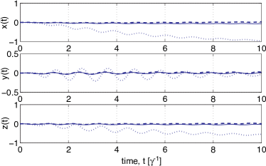
Figure 2: This figure depicts the difference between the reduced state calculated form our perturbative coherent non-Markovian SSE and the enlarged system method. The dotted line corresponds to the $0^{\rm th}$ order perturbation, the dashed is the $1^{\rm st}$ and the solid is the $2^{\rm nd}$. Other details are as in Fig. 1.

V.4 Quadrature Unravelling-TLA

For the quadrature unravelling the actual non-Markovian SSE is

$$d_{t}|{\psi_{z}({t})}\rangle = \Big{[}-i\frac{\Delta}{2}\hat{\sigma}_{z}-i\frac{\chi}{2}\hat{\sigma}_{x}-(\hat{\sigma}_{x}-\langle\hat{\sigma}_{x}\rangle_{t})~{}^{(0)}\hat{Q}_{z}(t)$$ (127)

$$+\Big{\langle}(\hat{\sigma}_{x}-\langle\hat{\sigma}_{x}\rangle_{t})~{}^{(0)}\hat{Q}_{z}(t)\Big{\rangle}_{t}$$

$$+z(t)(\hat{\sigma}-\langle\hat{\sigma}\rangle_{t})\Big{]}|{\psi_{z}({t})}\rangle,$$

and the noise function for the TLA is

$$z(t)=z_{\Lambda}(t)+\int_{0}^{t}\beta{(t-s)}\langle\hat{\sigma}_{x}\rangle_{s}ds.$$ (128)

Again the coherent case we can calculate the complex amplitude equation via applying the state $|{\psi_{z}({t})}\rangle=C_{e}(t)|{e}\rangle+C_{g}(t)|{g}\rangle$ to Eq. (127) and expanding $~{}^{(0)}\hat{Q}_{z}(t)$ as

$$~{}^{(0)}\hat{Q}_{z}(t)=\sum_{m}\hat{m}~{}^{(0)}{Q}_{m,z}(t)$$ (129)

where $m=\{\sigma$, $\sigma^{\dagger}$, $\sigma_{z}$, $I\}$. This results in a coupled set of differential equations for $C_{e}(t)$ and $C_{g}(t)$ that depend on $~{}^{(0)}{Q}_{m,z}(t)$ and $z(t)$. In these equations the real-valued noise is given by

$$z(t) = z_{\Lambda}(t)+\frac{\gamma\kappa}{4}e^{-\kappa t/2}\int_{0}^{t}e^{\kappa s/2}[C_{g}(s)C^{*}_{e}(s)$$ (130)

$$+C^{*}_{g}(s)C_{e}(s)]ds,$$

where $z_{\Lambda}(t)$ is found by

$$\tilde{{E}}[{z}_{\Lambda}(t)z_{\Lambda}(s)]=\frac{\gamma\kappa}{4}e^{-\kappa|t-s|/2}.$$ (131)

This is generated by

$$d_{t}z_{\Lambda}(t)=-\frac{\kappa}{2}z_{\Lambda}(t)+\frac{\kappa}{2}\sqrt{\gamma}\,\xi(t)$$ (132)

with $z_{\Lambda}(0)$ being a GRV satisfying ${E}[z_{\Lambda}(0)z^{*}_{\Lambda}(0)]={\kappa\gamma}/{4}$. Here $\xi(t)$ is standard white noise and satisfies $E[\xi(t)\xi^{*}(s)]=\delta(t-s)$ Gar83 .

V.4.1 $0^{\rm th}$ Order Approximation

The situation is greatly simplified with the memory function in Eq. (100), as $\beta(t,s)=\beta^{(j,cos)}(t,s)=\beta^{(j,cos)}(t,s)$, which in turn implies $~{}^{(0)}\hat{Q}_{z}(t)=~{}^{(0)}\hat{Q}^{(j,\cos)}_{z}(t)=~{}^{(0)}\hat{Q}^{(j,\sin)}_{z}(t)$.

The $0^{\rm th}$ order approximation is to set

$$~{}^{(0)}\hat{Q}_{z}(t)=\frac{\gamma}{2}(1-e^{-\kappa t/2})\hat{\sigma},$$ (133)

thus

$$~{}^{(0)}{Q}_{\sigma,z}(t) = \frac{\gamma}{2}(1-e^{-\kappa t/2}),$$ (134a)

$$~{}^{(0)}{Q}_{\sigma^{\dagger},z}(t) = ~{}^{(0)}{Q}_{\sigma_{z},z}(t)=~{}^{(0)}{Q}_{I,z}(t)=0.$$ (134b)

V.4.2 $1^{\rm th}$ Order Approximation

The first order approximation is to set

$$~{}~{}^{(1)}\hat{Q}_{z}(t)=\frac{\gamma}{2}(1-e^{-\kappa t/2})[\hat{\sigma},~{}^{(0)}\hat{Q}_{z}(t)]$$ (135)

thus

$$~{}^{(1)}{Q}_{\sigma,z}(t) = {\gamma}(1-e^{-\kappa t/2})~{}^{(0)}{Q}_{\sigma_{z},z}(t),$$ (136a)

$$~{}^{(1)}{Q}_{\sigma_{z},z}(t) = -\frac{\gamma}{2}(1-e^{-\kappa t/2})~{}^{(0)}{Q}_{\sigma^{\dagger},z}(t),$$ (136b)

$$~{}^{(1)}{Q}_{\sigma^{\dagger},z}(t) = ~{}^{(1)}{Q}_{I,z}(t)=0.\hskip 22.76228pt$$ (136c)

The $0^{\rm th}$ order functionals are found by applying TLA operators to Eq. (84). With the simple memory function this gives

$$d_{t}~{}^{(0)}\hat{Q}_{z}(t) = \frac{\gamma\kappa}{4}\hat{\sigma}-\frac{\kappa}{2}~{}^{(0)}\hat{Q}_{z}(t)+z(t)[\hat{\sigma},~{}^{(0)}\hat{Q}_{z}(t)]$$ (137)

$$-i[\frac{\Delta}{2}\hat{\sigma}_{z}+\frac{\chi}{2}\hat{\sigma}_{x},~{}^{(0)}\hat{Q}_{z}(t)]$$

$$-[\hat{\sigma}_{x}~{}^{(0)}\hat{Q}_{z}(t),~{}^{(0)}\hat{Q}_{z}(t)]$$

$$-\hat{\sigma}_{x}~{}^{(1)}\hat{Q}_{z}(t).$$

Using Eq. (129) this gives,

$$d_{t}~{}^{(0)}{Q}_{\sigma,z}(t) = \mbox{$\frac{1}{4}$}\gamma\kappa-\frac{\kappa}{2}~{}^{(0)}{Q}_{\sigma,z}(t)+{i}\Delta~{}^{(0)}{Q}_{\sigma,z}(t)-{i}\chi~{}^{(0)}{Q}_{\sigma_{z},z}(t)+2z(t)~{}^{(0)}{Q}_{\sigma_{z},z}(t)+~{}^{(0)}{Q}^{2}_{\sigma,z}(t)$$ (138a)

$$-2~{}^{(0)}{Q}_{\sigma_{z},z}(t)[~{}^{(0)}{Q}_{I,z}(t)+~{}^{(0)}{Q}_{\sigma_{z},z}(t)]-~{}^{(0)}{Q}_{\sigma^{\dagger},z}(t)~{}^{(0)}{Q}_{\sigma,z}(t)$$

$$-[~{}^{(1)}{Q}_{I,z}(t)+~{}^{(1)}{Q}_{\sigma_{z},z}(t)],$$

$$d_{t}~{}^{(0)}{Q}_{\sigma^{\dagger},z}(t) = -\frac{\kappa}{2}~{}^{(0)}{Q}_{\sigma^{\dagger},z}(t)+{i}\chi~{}^{(0)}{Q}_{\sigma_{z},z}(t)-{i}\Delta~{}^{(0)}{Q}_{\sigma^{\dagger},z}(t)+2~{}^{(0)}{Q}_{\sigma_{z},z}(t)[~{}^{(0)}{Q}_{I,z}(t)-~{}^{(0)}{Q}_{\sigma_{z},z}(t)]$$ (138b)

$$-~{}^{(0)}{Q}_{\sigma^{\dagger},z}(t)~{}^{(0)}{Q}_{\sigma,z}(t)+~{}^{(0)}{Q}^{2}_{\sigma^{\dagger},z}(t)-~{}^{(1)}{Q}_{I,z}(t)+~{}^{(1)}{Q}_{\sigma_{z},z}(t),$$

$$d_{t}~{}^{(0)}{Q}_{\sigma_{z},z}(t) = -\frac{\kappa}{2}~{}^{(0)}{Q}_{\sigma_{z},z}(t)+i\frac{\chi}{2}~{}^{(0)}{Q}_{\sigma^{\dagger},z}(t)-i\frac{\chi}{2}~{}^{(0)}{Q}_{\sigma,z}(t)-~{}^{(0)}{Q}_{\sigma,z}(t)[~{}^{(0)}{Q}_{I,z}(t)-~{}^{(0)}{Q}_{\sigma_{z},z}(t)]$$ (138c)

$$+~{}^{(0)}{Q}_{\sigma^{\dagger},z}(t)[~{}^{(0)}{Q}_{I,z}(t)+~{}^{(0)}{Q}_{\sigma_{z},z}(t)]-z(t)~{}^{(0)}{Q}_{\sigma^{\dagger},z}(t)$$

$$-\mbox{$\frac{1}{2}$}[~{}^{(1)}{Q}_{\sigma,z}(t)-~{}^{(1)}{Q}_{\sigma^{\dagger},z}(t)],$$

$$d_{t}~{}^{(0)}{Q}_{I,z}(t) = -\frac{\kappa}{2}~{}^{(0)}{Q}_{I,z}(t)-\mbox{$\frac{1}{2}$}[~{}^{(1)}{Q}_{\sigma,z}(t)+~{}^{(1)}{Q}_{\sigma^{\dagger},z}(t)].$$ (138d)

which can be solved in parallel with $C_{e}(t)$ and $C_{g}(t)$.

To illustrate how accurate our perturbation method is for the quadrature unravelling. Fig. 3 shows the difference between the reduced state calculated via the enlarged system method and the ensemble average from the quadrature non-Markovian SSEs for the $0^{\rm th}$ (dotted) and $1^{\rm st}$ (dashed) order perturbation. As in the coherent case we find the $1^{\rm st}$ order perturbation is more accurate then the $0^{\rm th}$.

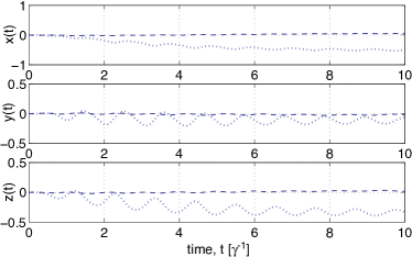
Figure 3: This figure depicts the difference between the reduced state calculated form our perturbative quadrature non-Markovian SSE and the enlarged system method. The dotted line corresponds to the $0^{\rm th}$ and the dashed is the $1^{\rm st}$ order perturbation. Other details are as in Fig. 1.

VI Post-Markovian perturbation

In this section we extend the YDGS post-Markovian perturbation YuDioGisStr99 to include the quadrature unraveling and compare the post-Markovian method with our perturbation method.

The basis idea behind their perturbation method is to expand the operators $~{}^{(0)}\hat{f}_{z}(t,s)$ in powers of $(t-s)$ around the point $t=s$ (this is why it is called the post Markovian perturbation). That is

$$~{}^{(0)}\hat{f}_{z}(t,s) = ~{}^{(0)}\hat{f}_{z}(s,s)+[\partial_{t}~{}^{(0)}\hat{f}_{z}(t,s)|_{t=s}](t-s)$$ (139)

$$+\mbox{$\frac{1}{2}$}[\partial^{2}_{t}~{}^{(0)}\hat{f}_{z}(t,s)|_{t=s}](t-s)^{2}+...,$$

where $~{}^{(0)}\hat{f}_{z}(s,s)=\hat{L}$. To find the first order term we simply evaluate Eq. (57) at $t=s$

$$\partial_{t}~{}^{(0)}\hat{f}_{z}(t,s)|_{t=s} = -\frac{i}{\hbar}[\hat{H}_{\rm int}(s),\hat{L}]-[\hat{L}^{\dagger}~{}^{(0)}\hat{F}_{z}(s),\hat{L}]$$ (140)

$$-\hat{L}^{\dagger}[\hat{L},~{}^{(0)}\hat{F}_{z}(s)].$$

Thus the functional $~{}^{(0)}\hat{F}_{z}(t)$ for this perturbation is given by

$$~{}^{(0)}\hat{F}_{z}(t) = g_{0}(t)\hat{L}-g_{1}(t)\frac{i}{\hbar}[\hat{H}_{\rm int}(t),\hat{L}]$$ (141)

$$-\int_{0}^{t}\alpha(t-s)(t-s)[\hat{L}^{\dagger}~{}^{(0)}\hat{F}_{z}(s),\hat{L}]ds$$

$$-\int_{0}^{t}\alpha(t-s)(t-s)\hat{L}^{\dagger}[\hat{L},~{}^{(0)}\hat{F}_{z}(s)]ds,\hskip 28.45274pt$$

where

$$g_{0}(t) = \int_{0}^{t}\alpha(t-s)ds,$$ (142)

$$g_{1}(t) = \int_{0}^{t}\alpha(t-s)(t-s)ds.$$ (143)

This equation can not be solved without the initial condition $d_{t}~{}^{(0)}\hat{F}_{z}(0)$. However if we make the approximate $~{}^{(0)}\hat{F}_{z}(s)=\int_{0}^{s}\alpha(s-u)\hat{L}du$, Eq. (141) becomes

$$~{}^{(0)}\hat{F}_{z}(t)=g_{0}(t)\hat{L}-g_{1}(t)\frac{i}{\hbar}[\hat{H}_{\rm int}(t),\hat{L}]-g_{2}(t)[\hat{L}^{\dagger}\hat{L},\hat{L}],$$ (144)

where

$$g_{2}(t)=\int_{0}^{t}\int_{0}^{s}\alpha(t-s)\alpha(s-u)(t-s)duds,$$ (145)

which can be solved. The same could be done for the second order terms, but as well as making an approximation for $~{}^{(0)}\hat{F}_{z}(s)$ we would need to approximate $d_{s}~{}^{(0)}\hat{F}_{z}(s)$. For the purpose of this paper we will only go to first order.

To extend the idea to the quadrature case we Taylor expand the operator $~{}^{(0)}\hat{q}_{z}(t,s)$ in powers of $(t-s)$ around the point $t=s$. To find the first order term we simply evaluate Eq. (83) at $t=s$. With the approximation $~{}^{(0)}\hat{Q}_{z}(s)=\int_{0}^{s}\beta(s-u)\hat{L}du$ we get

$$~{}^{(0)}\hat{Q}_{z}(t)=h_{0}(t)\hat{L}-h_{1}(t)\frac{i}{\hbar}[\hat{H}_{\rm int}(t),\hat{L}]-h_{2}(t)[\hat{L}_{x}\hat{L},\hat{L}].$$ (146)

where

$$h_{0}(t) = \int_{0}^{t}\beta(t-s)ds,$$ (147)

$$h_{1}(t) = \int_{0}^{t}\beta(t-s)(t-s)ds,$$ (148)

$$h_{2}(t) = \int_{0}^{t}\int_{0}^{s}\beta(t-s)\beta(s-u)(t-s)duds.$$ (149)

For the simple TLA system it is easy to generate these approximate expressions for $~{}^{(0)}\hat{F}_{z}(t)$ and $~{}^{(0)}\hat{Q}_{z}(t)$ for all time, hence we can obtain solution to the non-Markovian SSE. To compare YDGS post-Markovian non-Markovian SSE method with our perturbation method, we again plot the difference between YDGS method (when 1000 trajectories where used) and the enlarged systems method. The results of this are shown in Fig. 4, where it is observed that YDGS first order perturbation has a greater error than our perturbation method (Figs. 2 and 3). This is perhaps not surprising, as the system we modelled has $\kappa=1$, which implies it is very non-Markovian. Since one of the requirements of YDGS perturbation method is for the environment to be close the Markovian regime one would expect their method to fail in this regime.

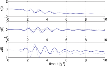
Figure 4: This figure shows the difference between the reduced state calculated from YDGS post-Markovian non-Markovian SSE method and the enlarged system method, for both the coherent (dotted line) and quadrature (solid line) unraveling. Other details are as in Fig. 1.

In Ref. YuDioGisStr99 YDGS suggest an alternative perturbation method. The functional operator $~{}^{(0)}\hat{F}_{z}(t)$, which equals $\bar{O}_{z}(t)$ in their notation, is expanded by the functional expansion

$$\bar{O}_{z}(t) = \bar{O}^{(0)}(t)+\int_{0}^{t}\bar{O}^{(1)}(t,v)z(v)dv+\int_{0}^{t}\int_{0}^{t}\bar{O}^{(2)}(t,v_{1},v_{2})z(v_{1})z(v_{2})dv_{1}dv_{2}+...$$ (150)

$$+\int_{0}^{t}...\int_{0}^{t}\bar{O}^{(n)}(t,v_{1},...,v_{n})z(v_{1})...z(v_{n})dv_{1}...dv_{n}+...,$$

It can be shown that one can establish a set of coupled differential equations for these operators provided $\alpha(t-s)$ is given by Eq. (47). To truncated this perturbation at $\bar{O}^{(n)}$ one has to assume a value $\bar{O}^{(n+1)}$. It turns out that for all operators $\bar{O}^{(n)}$ other then $\bar{O}^{(0)}$ the only reason the operators change from their initial value $0$ at $t=0$ is if the assumed $\bar{O}^{(n+1)}$ is nonzero. This suggest that this method is highly dependent on the assumed value for $\bar{O}^{(n+1)}$.

VII Conclusions

In this paper we presented a perturbation method for solving the coherent and quadrature non-Markovian SSEs. This perturbation method is easily extended to any order and is not limited to the post Markovian regime. However, the environment is restricted such that it has a correlation function satisfying Eq. (47). As shown in Ref. SteIma96 most non-Markovian environments can be simulated via this correlation function with a relative small $J$. This suggest that this perturbation method might be useful for simulating non-Markovian evolution for $\rho_{\rm red}(t)$.

One appealing feature of this method is that it provides a perturbative solution for $\rho_{\rm red}(t)$ which is positive by definition. However there is another method, namely Imamo$\bar{\rm g}$lu’s enlarged system method Ima94 ; SteIma96 , which provides a better solution for $\rho_{\rm red}(t)$. Imamo$\bar{\rm g}$lu’s enlarged system method requires fewer coupled differential equations to solve and the only approximation comes in by a truncation of the Hilbert space of the fictitious modes. As one increases the basis size for these modes this method will converge to the correct solution. By contrast, convergence has not been shown for our method.

This does not mean that our method is useless, as the primary interest in our method is not to simulate $\rho_{\rm red}(t)$, but to simulate the non-Markovian SSEs. This is interesting as a continuous in time interpretation of non-Markovian SSEs is not clear. In Ref. GamWis02 we showed that these non-Markovian SSE under standard quantum measurement theory do not have a continuous measurement interpretation. However Loubenets in Ref. Lou01 ; BarLou02 claimed that she has developed a new framework for continuous quantum measurements in which non-Markovian SSEs represent the evolution of a system state which is continuously monitored.

Future work on this topic is to look into this question. Another question that needs answering is whether it is possible to derive non-Markovian SSE based on a discrete basis such as photon number. We believe this question and the previous question will be related. Finally, there is the possible application of our method to strongly non-Markovian systems such as an atom laser HopMoyColSav00 or photon emission in a photonic bad-gap material Joh84 ; BayLamMol97 .

Appendix A Derivation of ${}^{(0)}\hat{f}_{z}(t,t)=\hat{L}$

To show that ${}^{(0)}\hat{f}_{z}(t,t)=\hat{L}$ we start by discretizing the functional derivative. We divide the range $[0,t)$ into $N$ intervals of width $\Delta t$, so the change in $|{\tilde{\psi}_{z}({t})}\rangle$ is

$$\delta|{\tilde{\psi}_{z}({t})}\rangle = \int_{0}^{t}\frac{\delta|{\tilde{\psi}_{z}({t})}\rangle}{\delta z^{*}(s)}\delta z^{*}(s)ds$$ (151)

$$= \sum_{i=0}^{N-1}\Delta t\Big{[}\frac{\partial|{\tilde{\psi}_{z}({t_{N}})}\rangle}{\partial z^{*}(t_{i})\Delta t}\Big{]}dz^{*}(t_{i}),$$

thus

$$\frac{\delta}{\delta z^{*}(s)}|{\tilde{\psi}_{z}({t})}\rangle=\frac{\partial|{\tilde{\psi}_{z}({t_{N}})}\rangle}{\partial z^{*}(t_{i})\Delta t},$$ (152)

if $s$ ($t_{i}$) is less than $t$ $(t_{N})$, which is the only situation we are interested in, then taking the limit that $s\rightarrow t$ ($t_{i}=t_{N-1}$) this becomes

$$\lim_{s\rightarrow t}\frac{\delta|{\tilde{\psi}_{z}({t})}\rangle}{\delta z^{*}(s)}=\frac{\partial[|{\tilde{\psi}_{z}({t_{N-1}})}\rangle+\Delta t\partial_{t}|{\tilde{\psi}_{z}({t_{N-1}})}\rangle]}{\partial z^{*}(t_{N-1})\Delta t}.$$ (153)

Discretizing Eq. (24) we get

$$\partial_{t}|{\tilde{\psi}_{z}({t_{N-1}})}\rangle = \Big{[}\frac{-i}{\hbar}\hat{H}_{\rm int}(t_{N-1})+z^{*}(t_{N-1})\hat{L}$$ (154)

$$-\hat{L}^{\dagger}\sum_{j=0}^{N-2}\alpha{(t_{N-1}-t_{j})}\frac{\partial}{\partial z^{*}(t_{j})}\Big{]}$$

$$\times|{\tilde{\psi}_{z}({t_{N-1}})}\rangle.$$

Substituting this into Eq. (153) and using the fact that the state at time $t_{N-1}$ only depends on the noise at time less then $t_{N-1}$, we get the limit

$$\frac{\delta|{\tilde{\psi}_{z}({t})}\rangle}{\delta z^{*}(t)}\rightarrow\hat{L}|{\tilde{\psi}_{z}({t})}\rangle.$$ (155)

Thus by Eq. (25) $~{}^{(0)}\hat{f}_{z}(t,t)=\hat{L}$.

References

- (1) S. Nakajima, Prog. Theor. Phys. 20, 948 (1958).
- (2) R. Zwanzig, J. Chem. Phys. 33, 1338 (1960).
- (3) W.H. Lindblad, Commun. Math. Phys. 48, 199 (1976).
- (4) C.W. Gardiner and P. Zoller Quantum noise (Springer-Verlag, Berlin, 2000).
- (5) J. Dalibard, Y. Castin and K. Mølmer, Phys. Rev. Lett. 68, 580 (1992).
- (6) C.W. Gardiner, A.S. Parkins and P. Zoller, Phys. Rev. A 46, 4363 (1992).
- (7) H.J. Carmichael, An Open Systems Approach to Quantum Optics (Springer-Verlag, Berlin, 1993).
- (8) A.G. Redfield, Adv. Magn. Reson. 1, 1 (1965). A (2002).
- (9) L. Diósi, Quantum Semiclass. Opt. 8, 309 (1996).
- (10) L. Diósi and W.T. Strunz, Phys. Lett. A 235, 569 (1997).
- (11) L. Diósi, N. Gisin and W.T. Strunz, Phys. Rev. A 58, 1699 (1998).
- (12) W.T. Strunz, L. Diósi and N. Gisin, Phys. Rev. Lett. 82, 1801 (1999).
- (13) W.T. Strunz, Chemical Physics 268, 237 (2001).
- (14) J.D. Cresser, Laser Phys. 10, 1 (2000).
- (15) A.A. Budini, Phys. Rev. A 63, 012106 (2000)
- (16) J. Gambetta and H.M. Wiseman, to be published in Phys. Rev. A (2002).
- (17) T. Yu, L. Diósi, N. Gisin and W.T. Strunz, Phys. Rev. A 60, 91 (1999).
- (18) T. Yu, L. Diósi, N. Gisin and W.T. Strunz, Phys. lett. A 265, 331 (2000).
- (19) A. Imamolu, Phys. Rev. A 50, 3650 (1994).
- (20) P. Stenius and A. A. Imamolu, Quantum Semiclass. Opt. 8, 283 (1996).
- (21) A. Bassi and G.C. Ghirardi, Phys. Rev. A 65, 042114 (2002)
- (22) E. R. Loubenets, J. Phys. A:Math. Gen. 34, 7639 (2001)
- (23) O.E. Barndorff-Nielsen and E. R. Loubenets, J. Phys. A:Math. Gen. 35, 565 (2002)
- (24) C. Cao, W. Long, J. Wei and H. Cao, Phys. Rev. A 64, 043810 (2001).
- (25) C.W. Gardiner and M.J. Collett, Phys. Rev. A 31, 3761 (1985).
- (26) C.W. Gardiner, Handbook of Stochastic Methods: for Physics, Chemistry and the Natural Science (Springer-Verlag, Berlin, 1983).
- (27) J.J. Hope, G.M. Moy, M.J. Collett, and C.M. Savage, Phys. Rev. A 61, 023603 (2000).
- (28) S. John, Phys. Rev. Lett. 53, 2169 (1984).
- (29) S. Bay, P. Lambropoulos, and K. Mølmer, Phys. Rev. Lett. 79, 2654 (1997).