Classical Dynamics as Constrained Quantum Dynamics

Abstract

We show that the classical mechanics of an algebraic model are implied by its quantizations. An algebraic model is defined, and the corresponding classical and quantum realizations are given in terms of a spectrum generating algebra. Classical equations of motion are then obtained by constraining the quantal dynamics of an algebraic model to an appropriate coherent state manifold. For the cases where the coherent state manifold is not symplectic, it is shown that there exist natural projections onto classical phase spaces. These results are illustrated with the extended example of an asymmetric top.

I Introduction

The observables of a finite dimensional Lie algebra of an algebraic system (defined below) are quantized by construction of an irreducible unitary representation of that Lie algebra, in accordance with Dirac’s prescription diracbook . Moreover, as discussed in two previous papers scalar ; vector , this quantization is achieved in a simple and highly practical way by coherent state and vector coherent state methods which, together with the theories of induced representations mackey and geometric quantization kostant ; souriau ; woodhouse , provide simple and powerful techniques for quantizing complex systems. However, it is also known that the quantization of observables that do not belong to a subalgebra of the infinite-dimensional Lie algebra of all observables is impossible by Dirac’s prescription joseph . Even for observables belonging to the universal enveloping algebra of a finite-dimensional algebra of observables, there is the so-called “ordering ambiguity”. The method of geometric quantization provides an elegant prescription for quantizing certain observables (those that preserve a polarization), but does not provide quantizations for all observables. In this paper, we start from the premise that the fundamental dynamics of physical systems are given by quantum mechanics and proceed to show that the classical mechanics of an algebraic system are implied by its quantizations. This result shows how classical mechanics can be defined within quantum mechanics and establishes rules for the inverse process of quantization. Thus, we suggest that a criterion for a valid quantization is that it should be consistent with dequantization. A related but distinct problem is the one of explaining why most macroscopic systems are observed to behave classically; however, we do not address this problem.

Our starting point is the observation that a quantal Hilbert space is a symplectic manifold and quantum mechanics is Hamiltonian mechanics on such a manifold. It is also known that restricting Dirac’s time-dependent variational principle,

$$\delta\int\langle\psi(t)|\Big{(}\hat{H}-i\hbar\frac{\partial}{\partial t}\Big{)}|\psi(t)\rangle\,{\rm d}t=0\,,$$ (1)

to a symplectic submanifold of the Hilbert space gives rise to Hamiltonian equations of motion on that submanifold. Approximate Hartree–Fock theories (cf. references cited in rowebook ), theories of large amplitude collective motion TDHF ; rowe80 and the density dynamics of Rowe, Vassanji and Rosensteel rowe83 have utilized this property of quantum systems extensively. Indeed many approximate many–body theories are known (cf. rowe80 ) to be expressible in terms of Hamiltonian equations in a classical form on symplectic submanifolds of the many–body Hilbert space. Hartree–Fock theory, time–dependent Hartree–Fock theory, the random–phase approximation, and the double–commutator equations–of–motion method rowebook are all describable in this context. Thus, given a Hilbert space for a quantum system, corresponding Hamiltonian equations of motion are defined by an embedding of a symplectic phase space in this Hilbert space as a submanifold and constraining the quantal dynamics to this submanifold. In this paper, we show that quantum mechanics constrained to an appropriate submanifold can lead to classical equations of motion, and evolution of observables consistent with the corresponding classical model.

For models with an algebraic structure, there is a straightforward and transparent means to define corresponding quantal and classical realizations using a spectrum generating algebra (SGA) scalar . It is shown in this paper that classical phase spaces for an algebraic model are embedded in its quantal representations. This embedding leads to a kinematical relationship between the symplectic structures of the classical and quantum models. The embeddings are often given by coherent state submanifolds of the quantal Hilbert space in a generalization of the well-known coherent states of the harmonic oscillator. In addition to the kinematical relationships given by such embeddings, we show that constraining quantum dynamics to an appropriate coherent state submanifold leads to classical equations of motion for all the observables of the model; i.e., classical dynamics is obtained as constrained quantum dynamics. For coherent state manifolds that are not symplectic, we consider their natural projections onto classical phase spaces. Thus, we show that it is possible to regain the classical dynamics of a model from its quantizations. This result goes beyond Ehrenfest’s theorem Ehr27 ; Bal94 to give classical equations of motion in terms of a classical Hamiltonian for all observables.

A potential ambiguity that arises is that there are many possible embeddings of a classical phase space in a given Hilbert space. It is then important to enquire if different but equally reasonable embeddings might give different classical dynamics. We show that the embedding problem is related to determining which quantal state of a system is most appropriately assigned to a classically observed state. Rather than a pure state, it seems natural to assign some mixture of states, such as a thermal distribution with expectations of the observables having values defined with distributions commensurate with those observed. However, with incomplete knowledge of a system, it is clear that specification of its quantal state cannot be unique. Thus, if the classical dynamics that emerge from different choices were to depend sensitively on the choice, it would be ambiguous. It is suggested in this paper by analyses of model systems that, while the various classical dynamics given by constrained quantum mechanics are not unique, they are nevertheless consistent with a single ideal classical mechanics defined as follows.

In an ideal classical mechanics, a point of the phase space is identified with a state of a system whose observables (e.g., position and momentum coordinates) all have precisely defined values. If quantum mechanics is fundamental, this description must be an idealization because it does not accurately describe any physical system obeying the uncertainty principle. Thus, a realistic classical description of a system should represent a state by a probability distribution of ideal classical states Bal94 , with mean values and variances that reflect these (classical) uncertainties. Each state in the probability distribution of ideal classical states would then evolve in accordance with the idealized classical mechanics so that, in any given situation, there would be a distribution of possible outcomes. We shall refer to such a dynamics as the physical classical dynamics.

It is of fundamental interest for the interpretation of quantum mechanics to be aware that many of its superficial differences with classical mechanics result from comparing it with the ideal rather than a physical version of the classical theory. The familiar example of a playing card balanced on one end on a flat table illustrates this point Teg01 . According to ideal classical mechanics, the card is in an equilibrium configuration and in the absence of interactions with its environment (e.g., air currents), it should remain in this configuration indefinitely. However, in quantum mechanics, its wave function is not in a stationary state and it will evolve symmetrically in such a way that the card is predicted to fall, with equal probability, to one side or the other. Exactly the same conclusion is reached in a physical classical analysis in which the initial state of the card is described by a symmetrical distribution of configurations about equilibrium. We do not suggest that quantum and classical mechanics necessarily give similar results, but simply stress that it is only meaningful to compare a physical classical mechanics with a fundamentally quantum description.

This paper is structured as follows. Sec. II presents the familiar example of barrier penetration to illustrate the concepts of ideal and physical classical dynamics, and how they relate to quantum and constrained quantum dynamics. In Sec. III, we introduce a description of both quantum and classical algebraic models in terms of an SGA, and formulate the concept of densities to describe a state of the classical system. In Sec. IV, we investigate how constraining the dynamics to appropriate coherent state manifolds can lead to classical equations of motion. These techniques are illustrated in Sec. V with a nontrivial application to the dynamics of an asymmetric top. Conclusions are presented in Sec. VI.

II Example: Barrier penetration

Barrier penetration is often used to illustrate the differences between classical and quantum mechanics. In this section, we use a barrier penetration example to introduce the essential concepts and principles that will be developed in the remainder of the paper.

We consider a point particle in one dimension, with Hamiltonian

$${H}=\frac{{p}^{2}}{2m}+{V}\,,$$ (2)

containing a potential energy defined by

$$V(x)=\begin{cases}V_{0}\quad&0\leq x\leq L\,,\\ 0&{\rm otherwise}\,,\end{cases}$$ (3)

where $V_{0}$ and $L$ are positive real numbers. For simplicity, we work in units in which $\hbar^{2}/2m=1$ and, in these units, set the barrier height to $V_{0}=1$. The momentum of the particle is then $p=\hbar k$, where $k$ is the wave number, and the energy of the particle, when outside of the barrier, is its kinetic energy $E(k)=k^{2}$.

II.1 Ideal versus physical states in classical mechanics

In ideal classical mechanics, the state of a particle in this system is represented as a point of position $x$ and momentum $p$ in a classical $(x,p)$ phase space.

In a description that more accurately represents a physical classical system, a state of the particle is represented by a probabililty distribution $P^{\rm CM}(\bar{x},\bar{k};x,k)$ of ideal classical states having mean position and momentum, given by

$$\bar{x} =\langle x\rangle=\int xP^{\rm CM}(\bar{x},\bar{k};x,k)\,{\rm d}x\,{\rm d}k\,,$$

$$\bar{p} =\langle\hbar k\rangle=\int\hbar kP^{\rm CM}(\bar{x},\bar{k};x,k)\,{\rm d}x\,{\rm d}k\,,$$ (4)

and corresponding variances in these means

$$\sigma^{2}(\bar{x}) =\int(x-\bar{x})^{2}P^{\rm CM}(\bar{x},\bar{k};x,k)\,{\rm d}x\,{\rm d}k\,,$$

$$\sigma^{2}(\bar{p}) =\int(\hbar k-\bar{p})^{2}P^{\rm CM}(\bar{x},\bar{k};x,k)\,{\rm d}x\,{\rm d}k\,.$$ (5)

To be specific, we consider classical probability distribution functions given by

$$P^{\rm CM}_{\alpha}(\bar{x},\bar{k};x,k)=\frac{1}{\pi}e^{-(x-\bar{x})^{2}/\alpha}e^{-\alpha(k-\bar{k})^{2}}\,.$$ (6)

for various values of $\alpha$. With physical states characterized by such distributions, the measured values of observables, such as the potential energy $V$, would have expectation values given, for example, by

$$\bar{V}_{\alpha}(\bar{x})=\int V(x)\,P^{\rm CM}_{\alpha}(\bar{x},\bar{k};x,k)\,{\rm d}x\,{\rm d}k\,,$$ (7)

and there would be corresponding uncertainties in these measured values due both to the errors of the measuring apparatus as well as the fundamental uncertainties in the position of the particle in a distribution of ideal states. As an illustration, Fig. 1 shows that expectation values of the potential barrier for the classical probability distribution functions given by Eq. (6) for various values of $\alpha$.

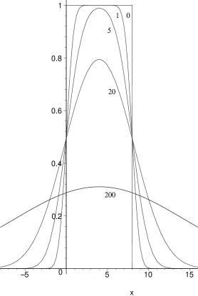
Figure 1: Expectations values $\bar{V}_{\alpha}$, defined by Eq. (7), of the potential, Eq. (3), for physical classical states having Gaussian probability distributions in position and momentum defined by Eq. (6) with various values of $\alpha$. The same expectation values are obtained for minimal uncertaintly quantum mechanical states with wave functions given by Eq. (10).

It should be noted that the classical probability distribution $P^{\rm CM}_{\alpha}(\bar{x},\bar{k};x,k)$ represents a physical state having the minimal product of uncertainties in position and momentum allowed by quantum mechanics. In general, physical states have much greater products of uncertainties.

The accuracy in the measurement of an observable function of position can be increased without limit, in principle, by admitting a correspondingly larger uncertainty in momentum. Thus, by letting $\alpha\to 0$, there is no limit in principle on the accuracy with which the potential energy or some other single observable can be measured. However, one cannot simultaneously measure the values of different (non-commuting) observables that depend on both the position and the momentum of the particle to greater precision than allowed by the uncertainty principle in any system with a fundamentally quantum description.

II.2 Constrained and unconstrained states in quantum mechanics

A state $|\psi\rangle$ of a particle in quantum mechanics defines probability distributions in the position and momentum variables given, respectively, by the square moduli of its wave functions $|\psi(x)|^{2}=|\langle x|\psi\rangle|^{2}$ and $|\varphi(k)|^{2}=|\langle k|\psi\rangle|^{2}$ in position and momentum representations. In particular, the mean values and variances of the position and momentum variables in a state $|\psi\rangle$ are given by

$$\bar{x}=\langle\psi|\hat{x}|\psi\rangle\,,\quad\sigma^{2}(\bar{x})=\langle\psi|(\hat{x}-\bar{x})^{2}|\psi\rangle\,,$$ (8)

and

$$\bar{p}=\langle\psi|\hat{p}|\psi\rangle\,,\quad\sigma^{2}(\bar{p})=\langle\psi|(\hat{p}-\bar{p})^{2}|\psi\rangle\,,$$ (9)

where $\hat{x}$ and $\hat{p}$ are the quantal position and momentum operators; in the position representation, they are given by $\hat{x}=x$ and $\hat{p}=-i\hbar\partial/\partial x$.

In constrained quantum mechanics, the dynamics is restricted to a submanifold of states distinguished by their mean values of $\bar{x}$ and $\bar{p}=\hbar\bar{k}$. A particular submanifold can be selected in many ways. For illustrative purposes, we consider here a set of minimum uncertainty states $\{|\alpha,\bar{x},\bar{k}\rangle\}$ (of fixed $\alpha$) with wave functions $\{\psi(\alpha,\bar{x},\bar{k})\}$ in the position representation

$$\psi(\alpha,\bar{x},\bar{k};x)=(\pi\alpha)^{-1/4}e^{-(x-\bar{x})^{2}/2\alpha}e^{i\bar{k}x}\,.$$ (10)

These wave functions have probability distribution in $x$ given by

$$P^{\rm QM}_{\alpha}(\bar{x};x)=\frac{1}{\sqrt{\pi\alpha}}e^{-(x-\bar{x})^{2}/\alpha}\,.$$ (11)

The corresponding wave functions in the momentum representation are given by the Fourier transforms

$$\varphi(\alpha,{\bar{x}},\bar{k};k)=(\alpha/\pi)^{1/4}e^{-\alpha(k-\bar{k})^{2}/2}e^{-i\bar{x}k}\,.$$ (12)

Hence, the probability distributions in momentum $p=\hbar k$ are given for these states by

$$P^{\rm QM}_{\alpha}(\bar{k};k)=\sqrt{\frac{\alpha}{\pi}}\,e^{-\alpha(k-\bar{k})^{2}}\,.$$ (13)

It is seen that the products of these distributions are identical to the classical distributions of Eq. (6), i.e.,

$$P^{\rm CM}_{\alpha}(\bar{x},\bar{k};x,k)=P^{\rm QM}_{\alpha}(\bar{x};x)P^{\rm QM}_{\alpha}(\bar{k};k)\,.$$ (14)

Thus, the expectation values of, for example, the potential energy in a state $|\alpha,\bar{x},\bar{k}\rangle$ are given by Eq. (7) with $P^{\rm CM}(\bar{x},\bar{k};x,k)=P^{\rm QM}_{\alpha}(\bar{x};x)P^{\rm QM}_{\alpha}(\bar{k};k)$.

This example illustrates the fact that a suitably selected set of constrained quantum mechanical states can give precisely the same mean values and variances as a corresponding set of physical classical states. It also makes clear that in suitable situations, e.g. when the Hamiltonian is a sum of a potential energy that is a function of only position coordinates and a kinetic energy that is a function of only momenta, it is possible (at least in principle) to probe the functional forms of the components of the Hamiltonian separately in both physical classical mechanics and contrained quantum mechanics to any desired accuracy. The important conclusion is that by observations of the values of physical observables in quantum mechanics it is possible to make precisely the same inferences about the ideal classical expressions of observables, e.g. as functions of position and momentum, as is, in principle, possible in physical classical mechanics. Of course, it is fully recognized that such a claim is not established by consideration of a single example. However, we suggest that the validity of this claim should follow from a suitably precise definition of what is meant by physical classical states.

II.3 Barrier penetration in classical mechanics

We now illustrate the meaning of ideal and physical classical mechanics in the context of the barrier penetration example and then do the same for unconstrained and constrained quantum mechanics.

In ideal classical mechanics, the probability for penetration of the barrier by a particle approaching the barrier with a precisely defined momentum $\hbar k$ is simply

$$T_{\rm ICM}(k)=\begin{cases}1&{\rm if}\;k>1,\\ 0&{\rm if}\;k<1.\end{cases}$$ (15)

Thus, in a physical situation in which the incident particle state at time $t=0$ is in a distribution of ideal classical states given by a function $P^{\rm CM}_{\alpha}(\bar{x},\bar{k};x,k)$, the probability for penetration of the barrier is given by

$$T_{\rm CM}(\alpha,\bar{k})=\int P^{\rm CM}_{\alpha}(\bar{x},\bar{k};x,k)\,T_{\rm ICM}(k)\,{\rm d}x\,{\rm d}k\,.$$ (16)

Numerically integrated values for these barrier penetration probabilities are shown as functions of the wave number $k$, for different values of $\alpha$, in Fig. 2 for the particular case of a barrier of width $L=8$.

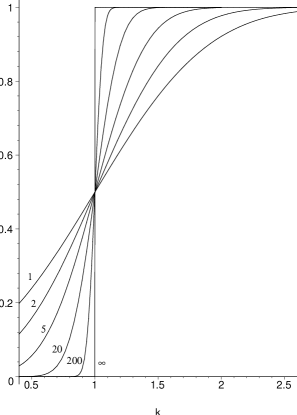
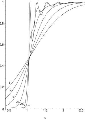
Figure 2: Transmission probabilities in physical classical mechanics (left) for Gaussian probability distributions in position and momentum defined, by Eqs. (6) and for corresponding minimal wave packets in quantum mechanics (right). The results are shown for a range of values of the Gaussian width parameter $\alpha$.

It is seen that, in the limit as $\alpha\to\infty$ and the momentum of the particle becomes precisely defined, the barrier penetration probability approaches that of ideal classical mechanics; this reflects the limiting value

$$\lim_{\alpha\rightarrow\infty}T_{\rm CM}(\alpha,k)=T_{\rm ICM}(k)\,.$$ (17)

II.4 Barrier penetration in quantum mechanics

In quantum mechanics, the probability for penetration of the barrier in the limit in which the incident particle is in a momentum eigenstate is given by

$$T_{\rm QM}(k)=\begin{cases}\displaystyle\frac{8k^{2}(k^{2}-1)}{8k^{2}(k^{2}-1)+1-\cos(2L(k^{2}-1))}{\rm if}\;k>1,\\ \displaystyle\frac{8k^{2}(k^{2}-1)}{8k^{2}(k^{2}-1)+1-\cosh(2L(1-k^{2}))}{\rm if}\;k<1.\end{cases}$$ (18)

This function is shown as the $\alpha=\infty$ curve on the right of Fig. 2 for a barrier of width $L=8$.

For a finite value of $\alpha$, the penetration probability for a particle in a state $|\alpha,\bar{x},\bar{k}\rangle$ at time $t=0$ is given by

$$T_{\rm QM}(\alpha,\bar{k})=\int T_{\rm QM}(k)P^{\rm QM}_{\alpha}(\bar{k};k)\,{\rm d}k\,.$$ (19)

The barrier penetration probabilities $T_{\rm QM}(\alpha,\bar{k})$ are shown for a range of value of $\alpha$ in Fig. 2. In parallel with the classical probabilities, the quantal penetration probabilities approach those for which the momentum is precisely defined in the $\alpha\to\infty$ limit.

It is notable that the quantal penetration probabilities have a remarkable resemblance to their classical counterparts. On examination, it is found that the classical penetration of the barrier exceeds that of quantum mechanics for all but a small region of $k\lesssim 1$. The remarkable feature of the quantal treatment is not so much the penetration of the barrier when the energy is less than would be required classically, as the reflection that occurs when the half wave length is an integer fraction of the barrier width.

II.5 Constrained quantum mechanics

Constrained quantum mechanics, as we define it in Sec. IV, gives the time evolution of a state subject to the constraint that it remains a coherent state at all times. As will be shown generally in this paper, the time evolution of the constrained wave function in the present example is of the form

$$\psi(x,t)=\psi(\alpha,{\bar{x}}(t),\bar{k}(t);x)\,e^{iE_{\alpha}t}\,,$$ (20)

where $\psi(\alpha,{\bar{x}},\bar{k};x)$ is given by Eq. (10) and $E_{\alpha}$ is the energy expectation of the coherent state. Thus, the time evolution of $\psi(x,t)$ is defined by the time evolutions of $\bar{x}(t)$ and $\bar{k}(t)$. We show, that $\bar{x}(t)$ and $\bar{p}(t)=\hbar\bar{k}(t)$ are given by classical dynamics for the Hamiltonian

$$H_{\alpha}(x,k)=\langle\psi(\alpha,x,k)|\hat{H}|\psi(\alpha,x,k)\rangle\,,$$ (21)

where $\hat{H}$ is the quantal Hamiltonian given by replacing the momentum $p$ in the classical expression (2) by the usual quantization $\hat{p}=-i\hbar{\rm d}/{\rm d}x$. One obtains

$$H_{\alpha}(x,k)=k^{2}+\bar{V}_{\alpha}(x)+{\rm const.}\,,$$ (22)

where the potential $\bar{V}_{\alpha}(x)$ is defined by Eq. (7). Thus, the probability for penetration of the barrier given by constrained quantum mechanics becomes identical to that of ideal classical mechanics provided the maximum value of the potential $\bar{V}(x)$ is the same as that for the original potential $V(x)$. The maxima are the same to a high degree of accuracy (cf. Fig. 1) for $\alpha\lesssim 2$ and become identical in the limit as $\alpha\to 0$, i.e., the limit in which the state $|\psi(\alpha,{\bar{x}},\bar{k})\rangle$ becomes an eigenstate of the position operator $\hat{x}$.

In a general situation, constrained quantum mechanics is governed by a Hamiltonian that is averaged, in parallel with Eq. (21), over the distributions of suitably defined coherent states for the system under consideration. Thus, in general, constrained quantum mechanics does not reproduce the original Hamiltonian precisely (except for the harmonic oscillator and limiting cases). But, by the same token, it is important to recognize that neither is the Hamiltonian of ideal classical mechanics reproduced exactly by physical classical mechanics except for similar limiting cases. Indeed, constrained quantum mechanics gives exactly the same Hamiltonian as physical classical mechanics when averaged over the same position and momentum distributions. That one does not reproduce the ideal classical Hamiltonian in either constrained quantum mechanics or in physical classical mechanics is a direct reflection of the limitation on observations imposed by the uncertainty principle.

Thus, while we cannot claim to derive the ideal classical mechanics of a system from its quantizations, we can claim to derive a classical mechanics that is consistent with the ideal classical mechanics in a sense that is similar to the way that physical classical mechanics is consistent with, but not identical to, ideal classical mechanics.

We consider these limitations in deriving the ideal classical dynamics of a system from quantum mechanics to be fundamental and to reflect the physics of the uncertainty principle. In particular, we claim that any inferences about relationships between observables that can be obtained by physical measurement can also be inferred as precisely as the uncertainty principle allows by quantum mechanical considerations.

III Classical and quantum algebraic models

In this section, we review the background material for describing an algebraic model, both classically and quantally, with a focus on the kinematical structure. For further details on algebraic models, see scalar . Also, Marsden and Ratiu marsden94 provide details on coadjoint orbits, Hamiltonian actions, and Hamiltonian formulations of quantum mechanics.

III.1 Observables and spectrum generating algebras

In classical mechanics, observables are realized as smooth real–valued functions on a connected phase space $\mathcal{M}$, i.e., elements of $C^{\infty}(\mathcal{M})$. They form an infinite–dimensional Lie algebra with Lie product given by a Poisson bracket. In quantum mechanics, observables are interpreted as Hermitian linear operators on a Hilbert space $\mathbb{H}$; they are elements of $GL(\mathbb{H})$ and form an infinite–dimensional Lie algebra with Lie product given by commutation.

The algebras $C^{\infty}(\mathcal{M})$ and $GL(\mathbb{H})$ for a given physical system are different joseph . However, for an algebraic system (defined below) it is possible to establish a simple relationship between finite–dimensional subalgebras of $C^{\infty}(\mathcal{M})$ and $GL(\mathbb{H})$. Let $\mathfrak{g}$ denote an abstract Lie algebra of observables that is real and finite–dimensional. Suppose that $\mathfrak{g}$ can be represented classically by a homomorphism $J:\mathfrak{g}\to C^{\infty}(\mathcal{M})$ and quantum mechanically by a unitary representation $T:\mathfrak{g}\to GL(\mathbb{H})$. Let $\mathcal{A}=J(A)$ and $\hat{A}=T(A)$ denote the classical and quantal representations, respectively, of an element $A\in\mathfrak{g}$. Then, if elements $A$, $B$, and $C\in\mathfrak{g}$ satisfy the commutation relations

$$[A,B]=i\hbar\,C\,,$$ (23)

the corresponding linear operators and functions satisfy

$$[\hat{A},\hat{B}]=i\hbar\,\hat{C}\,,$$ (24)

and

$$\{\mathcal{A},\mathcal{B}\}=\mathcal{C}\,,$$ (25)

where $\{\;,\;\}$ denotes the classical Poisson bracket. (More precisely, the homomorphism is given by $\{(i\hbar\mathcal{A}),(i\hbar\mathcal{B})\}=i\hbar(i\hbar\mathcal{C})$.)

It should be emphasized that the presence of the $i\hbar$ factor in the commutation relation, Eq. (23), of the abstract algebra has no quantum mechanical implications. The factor $\hbar$, for example, can be regarded simply as a suitable unit, chosen such that the Lie bracket $[A,B]$ has the same dimensions (i.e., is expressed in the same units) as a simple product of $A$ and $B$. The Poisson bracket, which differentiates, e.g., with respect to $x$ and $p$, does not have this property. The factor $i\hbar$ of the Lie bracket can be removed by simply dividing each of $A$, $B$ and $C$ by $i\hbar$. The dependence on $\hbar$ (equivalent to setting $\hbar=1$) can also be removed by expressing the observables in any convenient dimensionless units.

Let $\mathcal{G}\subset C^{\infty}(\mathcal{M})$ denote the classical algebra $\mathcal{G}=\{J(A)|A\in\mathfrak{g}\}$. If the values of the observables in $\mathcal{G}$ are sufficient to uniquely identify a point in $\mathcal{M}$, the algebra $\mathcal{G}$ (or $\mathfrak{g}$) is said to be a spectrum generating algebra (SGA) for the classical system ihrig . The Lie algebra $\mathfrak{g}$ is said to be a SGA for a quantal system if the Hilbert space for the system carries a unitary irreducible representation of $\mathfrak{g}$ SGA . A model dynamical system having a finite–dimensional SGA is said to be an algebraic system scalar .

Note that the SGA does not necessarily include the Hamiltonian. In fact, in a generic situation, the Hamiltonian is not an element of the SGA. To be useful, one may require that the Hamiltonian and other important observables of the system should be simply expressible in terms of $\mathfrak{g}$, e.g., by belonging to its universal enveloping algebra.

It is tempting to infer from the above considerations that the desired maps between the classical and quantal realizations of an algebraic system are simply Lie algebra homomorphisms. This idea underlies Dirac’s canonical quantization diracbook . However, these realizations do not give a complete description of the relationship between a quantum and classical model. In the first place, there may be many classical and many quantal representations of a given SGA but only some quantal representations qualify as quantizations of a given classical representation, and vice versa. Moreover, as proven by the famous Groenwald–van Hove theorem (see gotay ), the full algebra of classical observables has no irreducible representations.

III.2 Classical phase spaces as coadjoint orbits

The phase space of a classical algebraic model is naturally viewed as a coadjoint orbit of a dynamical group. Coadjoint orbits are mathematical constructions that have been widely studied and are known to have many useful properties marsden94 . In particular, they are known to be symplectic manifolds. For further details of the following construction, see scalar .

Let $G$ be a group of canonical transformations of a phase space $\mathcal{M}$ for a classical model. Then, if $G$ acts transitively on $\mathcal{M}$, it is said to be a dynamical group for the model. If an element $g\in G$ sends a point $m\in\mathcal{M}$ to $m\cdot g\in\mathcal{M}$, then $\mathcal{M}$ is the group orbit

$$\mathcal{M}=\{m\cdot g\,|\,g\in G\}$$ (26)

and diffeomorphic to the factor space $H_{m}\backslash G$ with isotropy subgroup

$$H_{m}=\{h\in g\,|\,m\cdot h=m\}\,.$$ (27)

A remarkable fact marsden94 that will be used extensively in the following is that a phase space with a dynamical group $G$ can be identified with a coadjoint orbit of $G$. Conversely, every coadjoint orbit is a phase space. Moreover, the Lie algebra $\mathfrak{g}$ of $G$ is a SGA for the model.

Recall that $G$ has a natural adjoint action on its Lie algebra $\mathfrak{g}$

$${\rm Ad}(g):\mathfrak{g}\to\mathfrak{g};\ A\mapsto A(g)={\rm Ad}(g)A\,,$$ (28)

where, for a matrix group, ${\rm Ad}(g)A=gAg^{-1}$. $G$ also has a coadjoint action on the space $\mathfrak{g}^{*}$ of real–valued linear functionals on $\mathfrak{g}$ (the dual of $\mathfrak{g}$). Thus, if $\rho$ is an element of $\mathfrak{g}^{*}$ and $\rho_{g}$ is defined by

$$\rho_{g}(A)=\rho(A(g))\,,\quad\forall\,A\in\mathfrak{g}\,,$$ (29)

then the coadjoint orbit

$$\mathcal{O}_{\rho}=\{\rho_{g}\,|\,g\in G\}\,,$$ (30)

is diffeomorphic to the factor space $H_{\rho}\backslash G$ with isotropy subgroup $H_{\rho}=\{h\in g\,|\,\rho_{h}=\rho\}$. We shall refer to an element $\rho$ of $\mathfrak{g}^{*}$ as a classical density. Now if a density $\rho\in\mathfrak{g}^{*}$ is chosen such that $H_{\rho}=H_{m}$ then there is a diffeomorphism $\mathcal{M}\to\mathcal{O}_{\rho}$ in which $m\mapsto\rho$ and $m\cdot g\mapsto\rho_{g}$. This map is known as a moment map.

The map $\mathcal{M}\to\mathcal{O}_{\rho}$ defines a classical representation $J:\mathfrak{g}\to\mathcal{G};A\mapsto\mathcal{A}=J(A)$ of the Lie algebra $\mathfrak{g}$ as functions over the classical phase space $\mathcal{M}$, defined by

$$\mathcal{A}(m\cdot g)=\rho_{g}(A)\,,$$ (31)

with Poisson bracket given by

$$\{\mathcal{A},\mathcal{B}\}=\sigma(A,B)\,,$$ (32)

where $\sigma$ is the antisymmetric two–form on the algebra with values at $m\cdot g\in\mathcal{M}$ given by

$$\sigma_{m\cdot g}(A,B)=-\frac{i}{\hbar}\,\rho_{g}([A,B])\,,\quad\forall\,A,B\in\mathfrak{g}\,.$$ (33)

This two–form is nondegenerate, and thus (with the realization of the Lie algebra $\mathfrak{g}$ as a set of invariant vector fields on $\mathcal{M}$) defines a symplectic form on $\mathcal{M}$.

The moment map $\mathcal{M}\to\mathcal{O}_{\rho}$ relates the symplectic structure of these spaces, making them symplectomorphic. Thus, $\sigma$ can be equivalently viewed as a symplectic form on either $\mathcal{M}$ or $\mathcal{O}_{m}$; they are equivalent as classical phase spaces. This powerful result allows us to interchange between the phase space $\mathcal{M}$ of an algebraic model and it’s corresponding coadjoint orbit $\mathcal{O}_{m}$; they are equivalent.

III.3 Quantum mechanics as Hamiltonian mechanics

A quantum system consists of a Hilbert space $\mathbb{H}$ and a set of observables, including a Hamiltonian $\hat{H}$, given as Hermitian linear operators in $GL(\mathbb{H})$. Quantum dynamics is given by the Schrödinger equation

$$i\hbar\frac{\partial}{\partial t}|\psi(t)\rangle=\hat{H}|\psi(t)\rangle\,,$$ (34)

for $|\psi(t)\rangle\in\mathbb{H}$. In this section, quantum dynamics is expressed as Hamiltonian dynamics relative to a natural symplectic form on the corresponding projective Hilbert space $\mathbb{PH}$. (A projective Hilbert space is a Hilbert space together with an equivalence relation which identifies vectors that are the same to within a complex factor. Thus, we say that $|\psi\rangle\equiv|\phi\rangle$ if $|\psi\rangle=c|\phi\rangle$ for some $c\in\mathbb{C}$.)

The complex Hermitian inner product of a Hilbert space leads to a Hermitian metric on the projective Hilbert space known as the Fubini-Study metric marsden94 . This metric provides two real non-degenerate bilinear forms on $\mathbb{PH}$. For $\mathbb{H}$ finite–dimensional, the first is defined in terms of a coordinate patch $\{\zeta^{\mu}\}$ by

$$g_{\mu\nu}(\psi)=g\big{(}\frac{\partial}{\partial\zeta^{\mu}},\frac{\partial}{\partial\zeta^{\nu}}\Big{)}(\psi)={\rm Re}\Bigl{\langle}\frac{\partial\psi}{\partial\zeta^{\mu}}\Bigl{|}\frac{\partial\psi}{\partial\zeta^{\nu}}\Bigr{\rangle}\,.$$ (35)

It is symmetric, hence Riemannian, and provides concepts of distance and curvature. The second,

$$\omega_{\mu\nu}(\psi)=\omega\big{(}\frac{\partial}{\partial\zeta^{\mu}},\frac{\partial}{\partial\zeta^{\nu}}\Big{)}(\psi)=-2\hbar\ \text{Im}\Bigl{\langle}\frac{\partial\psi}{\partial\zeta^{\mu}}\Bigl{|}\frac{\partial\psi}{\partial\zeta^{\nu}}\Bigr{\rangle}\,,$$ (36)

is anti-symmetric and closed; hence it is symplectic. The latter provides the basic structure whereby quantum mechanics can be expressed in Hamiltonian form.

If the Hilbert space $\mathbb{H}$ carries a unitary representation $T$ of a Lie group $G$, then the action of $G$ on $\mathbb{PH}$ leaves the Fubini–Study metric invariant marsden94 . Thus, $G$ acts on $\mathbb{PH}$ as a group of canonical transformations relative to the symplectic form $\omega$.

There exists a map from operators in $GL(\mathbb{H})$ to functions on $\mathbb{PH}$ in which $\hat{F}$ maps to a function $F$ on $\mathbb{PH}$ defined by its expectation value

$$F(\psi)=\langle{\psi}|{\hat{F}}|{\psi}\rangle\,.$$ (37)

With the energy function $H$ defined on $\mathbb{PH}$ by the expectation of the quantal Hamiltonian $\hat{H},$

$$H(\psi)=\langle{\psi}|{\hat{H}}|{\psi}\rangle\,,$$ (38)

and its derivatives expressed

$$\frac{\partial H}{\partial\zeta^{\nu}} =\left[\Bigl{\langle}\frac{\partial\psi}{\partial\zeta^{\nu}}\Big{|}\hat{H}{\psi}\Big{\rangle}+\Bigl{\langle}{\hat{H}\psi}\Big{|}\frac{\partial\psi}{\partial\zeta^{\nu}}\Big{\rangle}\right]$$

$$=i\hbar\left[\Bigl{\langle}\frac{\partial\psi}{\partial\zeta^{\nu}}\Big{|}\dot{\psi}\Big{\rangle}-\Bigl{\langle}{\dot{\psi}}\Big{|}\frac{\partial\psi}{\partial\zeta^{\nu}}\Big{\rangle}\right]\,,$$ (39)

with

$$\dot{\psi}=\frac{\partial\psi}{\partial\zeta^{\mu}}\dot{\zeta}^{\mu},$$ (40)

the time derivatives of the coordinates are determined rowe80 to be given by

$$\dot{\zeta}^{\mu}=\omega^{\mu\nu}\frac{\partial H}{\partial\zeta^{\nu}}\,.$$ (41)

Here, $\omega^{\mu\nu}$ is the inverse of the symplectic metric $\omega_{\mu\nu}$, defined by $\omega_{\mu\alpha}\omega^{\nu\alpha}=\delta_{\mu}^{\nu}$. Hence, the time evolution of $F$ is given by

$$\dot{F}=\{F,H\}_{\text{QM}}\,,$$ (42)

where the Poisson bracket of any two functions $F_{1},F_{2}$ on $\mathbb{PH}$ is defined by

$$\{F_{1},F_{2}\}_{\text{QM}}=\frac{\partial F_{1}}{\partial\zeta^{\mu}}\omega^{\mu\nu}\frac{\partial F_{2}}{\partial\zeta^{\nu}}\,.$$ (43)

This equation for the quantum Poisson bracket can be put into the coordinate–independent form

$$i\hbar\{F_{1},F_{2}\}_{\text{QM}}(\psi)=\langle\psi|[\hat{F_{1}},\hat{F_{2}}]|\psi\rangle$$ (44)

for any two functions $F_{1}(\psi)=\langle\psi|\hat{F}_{1}|\psi\rangle$ and $F_{2}(\psi)=\langle\psi|\hat{F}_{2}|\psi\rangle$ given by expectation values of operators. This expression of the Poisson bracket has the advantage that it applies to an infinite–dimensional Hilbert space. Moreover, the standard equation for time evolution in quantum mechanics,

$$\dot{F}(\psi)=-{\frac{i}{\hbar}}\langle\psi|[\hat{F},\hat{H}]|\psi\rangle\,,$$ (45)

again returns the classical–like expression

$$\dot{F}=\{F,H\}_{\text{QM}}\,.$$ (46)

Note that, although this Poisson bracket is of the same form as that of classical mechanics, it is defined on the whole projective Hilbert space $\mathbb{PH}$ whose only resemblance to a classical phase space is that it is a symplectic manifold; in particular, $\mathbb{PH}$ is generally infinite–dimensional whereas the corresponding classical phase space is finite.

These results show that there is a homomorphism from the (infinite) Lie algebra of all Hermitian linear operators on $\mathbb{H}$ to a corresponding Poisson bracket algebra of functions on a phase space. However, the resulting dynamics is not classical; as a phase space, the projective Hilbert space is generally too large. For the example of a single particle in one dimension, the Hilbert space is infinite–dimensional whereas the required classical phase space is two–dimensional. In the following section it is shown that, under certain conditions, the classical dynamics of an algebraic model can be realized on a submanifold of the projective Hilbert space. Such submanifolds are naturally realized as coherent state manifolds.

IV Classical mechanics as constrained quantum mechanics

To extract a mechanics from quantum mechanics that approximates ideal classical mechanics as closely as allowed by the uncertainty principle, it is appropriate to consider coherent state manifolds of minimal uncertainty states. However, while it is important to consider the limits of precision that are in principle attainable, it should be recognized that classical mechanics rarely deals with measurements at the level of quantum uncertainties. For example, in a situation in which classical mechanics is considered useful, it is rare that one could make a measurement of (say) the magnitude of a system’s angular momentum that would be sufficiently precise to distinguish its discrete quantized values. Thus, in situations where a classical description applies, it is not typically possible to identify a unique unitary irrep to which a given system might belong. Indeed, it is generally appropriate to characterize a system at a finite temperature by mixed states with contributions from different irreps.

We therefore consider two types of coherent state manifolds. We first consider the special case of a submanifold of pure states of the Hilbert space for an irrep of a dynamical group, and show that it is possible to constrain the quantal dynamics to such a submanifold, provided it is symplectic, and thereby obtain a classical dynamics. The second more general type of manifold we consider is a set of generalized coherent states comprising arbitrary mixed states described by density matrices. We show how classical dynamics is obtained generally for such a manifold.

IV.1 Coherent state submanifolds

Let $\mathfrak{g}$ be a SGA for an algebraic system, and $G$ a corresponding dynamical group with $\mathfrak{g}$ as its Lie algebra. Let $T$ be an irreducible unitary representation of $G$ on a Hilbert space $\mathbb{H}$; together with a Hamiltonian operator $\hat{H}$, this representation defines a quantal algebraic model. Any normalized state vector $|0\rangle\in\mathbb{H}$ defines a classical density $\rho_{m}$ for which

$$\rho_{m}(A)=\langle 0|\hat{A}|0\rangle,\quad\forall\ A\in\mathfrak{g}\,.$$ (47)

Since $G$ acts on $\mathbb{H}$ as a group of canonical transformations, there exists a moment map $|g\rangle\equiv T^{\dagger}(g)|0\rangle\to\rho_{m\cdot g}$, where

$$\rho_{m\cdot g}(A)=\langle g|\hat{A}|g\rangle=\rho_{m}(A(g))\,,$$ (48)

for all $A\in\mathfrak{g}$, with $A(g)$ defined by Eq. (28). Therefore, because a classical phase space is equivalent to an orbit $\mathcal{O}_{m}$ of the dynamical group $G$, it follows that the moment map takes every $G$–orbit in $\mathbb{PH}$

$$\mathcal{C}=\{|g\rangle=T^{\dagger}(g)|0\rangle;\ g\in G\}\,,$$ (49)

to a classical phase space

$$\mathcal{O}_{m}=\{\rho_{m\cdot g}\,;\,g\in G\}\,.$$ (50)

Orbits of $G$ in $\mathbb{PH}$ are known as systems of coherent states perelomov . Thus, every system of coherent states of a dynamical group defines a corresponding classical phase space and all its kinematical properties.

Note that the map $\mathcal{C}\to\mathcal{O}_{m}$ is kinematical; that is, it relates the two–form on $\mathcal{C}$, given by the restriction of the Fubini–Study metric of Eq. (36), to the classical symplectic structure on $\mathcal{O}_{m}$. However, if the map $\mathcal{C}\to\mathcal{O}_{m}$ is one-to-one, then with the addition of constraints, it also defines a classical Hamiltonian function $\mathcal{H}$ and a dynamics on $\mathcal{O}_{m}$.

Constraints are needed because, in general, the quantal time evolution of a coherent state does not remain a coherent state. The time evolution of a harmonic oscillator coherent state based on the harmonic oscillator ground state, which evolves classically under quantal time evolution, is an exception. Other exceptions arise for systems whose Hamiltonians lie in the SGA. Thus, in general, the quantal time evolution of a state that is initially a coherent state does not obey classical equations of motion. To obtain classical behaviour, it is necessary to constrain the quantal time evolution to prevent it from leaving the manifold of coherent states.

The theory of constrained Hamiltonian dynamics was first investigated by Dirac dirac64 and generalized in geometric terms by Gotay, Nester and Hinds gotaynesterhinds . Rowe, Ryman and Rosensteel rowe80 , for example, applied the theory of constraints to quantum systems and showed that Dirac’s time–dependent variational principle, Eq. (1), defines a Hamiltonian dynamics on any symplectic submanifold of $\mathbb{PH}$, i.e., a submanifold on which the restriction of the symplectic form $\omega$ is nondegenerate rowe80 ; rowe83 ; Kramer . We refer to such a Hamiltonian dynamics as constrained quantum mechanics. Thus, a classical Hamiltonian dynamics is defined by constraining quantum mechanics to any system of coherent states that is symplectic.

Let $\{z^{\nu}\}$ denote a set of coordinates for some neighbourhood in $\mathcal{C}$. Then, with the Hamiltonian function $H$ on $\mathcal{C}$ expressed as a function of these coordinates by

$$H(g(z))=\langle g(z)|\hat{H}|g(z)\rangle\,,$$ (51)

the derivatives of $H$ are given by

$$(\partial_{\mu}H)(g(z)) =\langle\partial_{\mu}g(z)|\hat{H}|g(z)\rangle+\langle g(z)|\hat{H}|\partial_{\mu}g(z)\rangle$$

$$=-\sigma_{\mu\nu}\dot{z}^{\nu}\,,$$ (52)

where $\partial_{\mu}\equiv\partial/\partial z^{\mu}$ and $\sigma$ is the restriction of the Fubini–Study symplectic form $\omega$ on $\mathbb{PH}$ to $\mathcal{C}$.

A special case occurs when $\mathcal{C}$ is symplectic. In this case, $(\sigma_{\mu\nu})$ can be inverted to give the (constrained) equations of motion

$$\dot{z}^{\mu}={\sigma}^{\mu\nu}(\partial_{\nu}H)\,,$$ (53)

with $(\sigma^{\mu\nu})$ defined such that

$$\sum_{\mu}\sigma^{\mu\nu}\sigma_{\mu\lambda}=\delta^{\nu}_{\lambda}\,.$$ (54)

These equations are equivalently obtained from Dirac’s variational principle. They are expressed in terms of Poisson brackets by observing that, for any function $F(z)\in C^{\infty}(\mathcal{C})$ on the coherent state orbit, the time evolution is given by

$$\dot{F}=(\partial_{\mu}F)\dot{z}^{\mu}=\{F,H\}_{\mathcal{C}}\,,$$ (55)

where

$$\{F,H\}_{\mathcal{C}}=(\partial_{\mu}F){\sigma}^{\mu\nu}(\partial_{\nu}H)\,.$$ (56)

If a coherent state submanifold $\mathcal{C}$ of $\mathbb{PH}$ is not symplectic then, as noted by Rowe et al. rowe80 , Dirac’s time-dependent variational principle does not define a constrained quantum dynamics on $\mathcal{C}$; the metric $(\sigma_{\mu\nu})$ does not have an inverse and Eq. (53) is not defined. However, even if not symplectic, $\mathcal{C}$ maps to a symplectic coadjoint orbit under the moment map. Moreover, it is possible to define a Hamiltonian function $\bar{H}$ on $\mathcal{O}$ as an average of $H$ over the states of $\mathcal{C}$ that map to a single classical state. Such an averaging process is defined and rationalized below. First, however, we note that if the map $\mathcal{C}\to\mathcal{O}$ is many–to–one, it cannot be inverted and, hence, no single quantal state in $\mathcal{C}$ is assigned to a given classical state in $\mathcal{O}$. This suggests that one should map a given classical state in $\mathcal{O}$ to a suitably defined mixture of the quantal states on $\mathcal{C}$ that cannot be distinguished by a measurement of classical observables rosensteelrowe81 , i.e., by the expectation values of elements in the SGA.

IV.2 Coherent manifolds of mixed states

Recall that a pure (normalized) state $|0\rangle$ in quantum mechanics can be represented by a quantal density (often called a density matrix) $\hat{\rho}_{0}=|0\rangle\langle 0|$ which maps to a classical density $\rho_{0}$, defined on the SGA of observables, by $\rho_{0}(A)={\rm Tr}(\hat{\rho}_{0}\hat{A})=\langle 0|\hat{A}|0\rangle$ for $A\in\mathfrak{g}$. Similarly, a mixed state is represented by a density $\hat{\rho}=\sum_{i}p_{i}|i\rangle\langle i|$, where $\{|i\rangle\}$ is a set of pure quantum states and $\{p_{i}\geq 0\}$ are coefficients of a probability distribution satisfying $\sum_{i}p_{i}=1$, and also gives a classical density $\rho$ defined by

$$\rho(A)={\rm Tr}(\hat{\rho}\hat{A})=\sum_{i}p_{i}\langle i|\hat{A}|i\rangle\,,$$ (57)

for $A\in\mathfrak{g}$.

To consider mixed states that span many irreps, we now allow $T$ to be a generally reducible unitary representation of $G$. Generalizing Eqs. (47) and (48), it is seen that an arbitrary density $\hat{\rho}$ for an algebraic system with dynamical group $G$ defines a corresponding manifold of mixed coherent states containing $\hat{\rho}$ given by

$$\mathcal{C}=\{\hat{\rho}_{g}=T(g^{-1})\hat{\rho}\,T(g),g\in G\}\,.$$ (58)

Moreover, there is a moment map, $\mathcal{C}\to\mathcal{O}_{m};\hat{\rho}_{g}\mapsto\rho_{m\cdot g}$, in which these coherent states map to a coadjoint orbit of classical densities with

$$\rho_{m\cdot g}(A)={\rm Tr}(\hat{\rho}_{g}\,\hat{A})=\sum_{i}p_{i}\langle i|T(g)\hat{A}T(g^{-1})|i\rangle\,,$$ (59)

for all $A$ in the SGA $\mathfrak{g}$ (the Lie algebra of $G$).

A density $\hat{\rho}_{g}$ has a natural interpretation as an element of the dual of the Lie algebra of linear operators on $\mathbb{H}$ with the standard pairing

$$\hat{\rho}_{g}:\hat{X}\to{\rm Tr}(\hat{\rho}_{g}\,\hat{X})\,.$$ (60)

The moment map, $\hat{\rho}_{g}\to\rho_{m\cdot g}$, is then seen as the restriction of $\hat{\rho}_{g}$ to the operators of the (generally reducible) unitary representation $T$ of the Lie algebra $\mathfrak{g}$ on $\mathbb{H}$, i.e., to $\{\hat{A}=T(A);A\in\mathfrak{g}\}$. It follows that the functions

$$\mathcal{A}(m\cdot g)={\rm Tr}(\hat{\rho}_{g}\,\hat{A})$$ (61)

and their Poisson brackets

$$\{\mathcal{A},\mathcal{B}\}(m\cdot g)=-\frac{i}{\hbar}\rho_{m\cdot g}([A,B])\,,$$ (62)

are well-defined on $\mathcal{O}_{m}$ for all $A,B\in\mathfrak{g}$. It also follows that any coherent state manifold of mixed (or pure) states defines a classical representation of $\mathfrak{g}$. This result is non-trivial because, in general, the coherent state manifold $\mathcal{C}$ is of higher dimension than the corresponding coadjoint orbit $\mathcal{O}_{m}$. As a result, the moment map does not preserve the commutation relations of arbitrary linear operators.

Being group orbits, $\mathcal{O}_{m}$ and $\mathcal{C}$ can be characterized as coset spaces. The coadjoint orbit $\mathcal{O}_{m}\simeq K_{\rho}\backslash G$ has stability subgroup

$$K_{\rho}=\{h\in G|{\rm Tr}(\hat{\rho}_{h}\,\hat{A})={\rm Tr}(\hat{\rho}\,\hat{A}),\;\forall A\in\mathfrak{g}\}\,,$$ (63)

whereas the stability subgroup for $\mathcal{C}\simeq K_{\hat{\rho}}\backslash G$ is

$$K_{\hat{\rho}}=\{h\in G|{\rm Tr}(\hat{\rho}_{h}\,\hat{X})={\rm Tr}(\hat{\rho}\,\hat{X})\}\,,$$ (64)

for any linear operator $\hat{X}$ that is bounded on $\mathcal{C}$.

To have a dynamics on $\mathcal{O}_{m}$, we need to know that the time-derivatives of the expectation values of the observables of $\mathfrak{g}$ at points of $\mathcal{C}$ defined according to the standard time-dependent Schrödinger equation by

$$\frac{{\rm d}}{{\rm d}t}{\rm Tr}(\hat{\rho}_{g}\,\hat{A})=-\frac{i}{\hbar}\,{\rm Tr}(\hat{\rho}_{g}\,[\hat{A},\hat{H}])\,,$$ (65)

map to well-defined functions on $\mathcal{O}_{m}$. It is seen that they do provided ${\rm Tr}(\hat{\rho}_{hg}\,[\hat{A},\hat{H}])$ is independent of $h$ for all $h\in K_{\rho}$ and all $A\in\mathfrak{g}$.

Claim: If $H(g)={\rm Tr}(\hat{\rho}_{g}\hat{H})$ satisfies $H(hg)=H(g)$, for all $h\in K_{\rho}$ and $g\in G$, then $\mathcal{H}(m\cdot g)=H(g)$ is a well-defined Hamiltonian on $\mathcal{O}_{m}$ and there is a well-defined Hamiltonian dynamics on $\mathcal{O}_{m}$ defined by

$$\dot{\mathcal{A}}(m\cdot g)=-\frac{i}{\hbar}\,{\rm Tr}(\hat{\rho}_{g}\,[\hat{A},\hat{H}])\,.$$ (66)

Proof: Define $\mathcal{H}(m)={\rm Tr}(\hat{\rho}\hat{H})$. Then, if ${\rm Tr}(\hat{\rho}_{h}\hat{H})={\rm Tr}(\hat{\rho}\hat{H})$ for all $h\in K_{\rho}$, we can define $\mathcal{H}(m\cdot g)={\rm Tr}(\hat{\rho}_{g}\hat{H})$ which is well-defined on $\mathcal{O}_{m}$. Now, assuming the conditions of the claim to be satisfied, we have

$$\mathcal{H}(m\cdot ge^{-\frac{i}{\hbar}aA})={\rm Tr}(\hat{\rho}_{g}e^{-\frac{i}{\hbar}aA}\hat{H}e^{\frac{i}{\hbar}aA})\,$$ (67)

with $a\in\mathbb{R}$ and $A\in\mathfrak{g}$. It follows that

$$-\frac{i}{\hbar}\,{\rm Tr}(\hat{\rho}_{g}\,[\hat{A},\hat{H}])=\frac{\partial\mathcal{H}}{\partial a}(m\cdot ge^{-\frac{i}{\hbar}aA})\Big{|}_{a=0}$$ (68)

is then well-defined on $\mathcal{O}_{m}$. QED

It is seen from the claim that the Hamiltonian on $\mathcal{C}$ automatically maps to a well-defined function on $\mathcal{O}_{m}$ in the special situation in which $K_{\rho}$ and $K_{\hat{\rho}}$ are the same and the manifolds $\mathcal{C}\simeq\mathcal{O}_{m}\simeq K_{\rho}\backslash G$ are diffeomorphic. In general, the Hamiltonian on $\mathcal{C}$ does not map directly to a well-defined function on $\mathcal{O}_{m}$, but it is now clear how to adjust the map so that it does. One can define a Hamiltonian on $\mathcal{O}_{m}$ as the average

$$\mathcal{H}(m\cdot g)=\bar{H}(g)=\frac{1}{v_{K_{\rho}}}\int_{K_{\rho}}H(hg)\,{\rm d}v(h)\,,$$ (69)

where ${\rm d}v$ is the left-invariant measure on $K_{\rho}$ and $v_{K_{\rho}}$ is the volume of $K_{\rho}$ with respect to this measure. (Note that the averaged energy function $\bar{H}(g)$ satisfies the condition of the claim that $\bar{H}(hg)=\bar{H}(g)$ for all $h\in K_{\rho}$.)

Such an averaging of $H$ is rationalized as follows. If the map $\mathcal{C}\to\mathcal{O}_{m}$ is many–to–one, it cannot be inverted. Hence, no unique quantal state (density) in $\mathcal{C}$ is assigned to a given classical state in $\mathcal{O}_{m}$. This multivaluedness suggests that to each classical state $\rho_{m\cdot g}\in\mathcal{O}_{m}$ one should assign a new quantal density $\hat{\rho}^{\prime}_{g}$ corresponding to a mixture with a suitable weighting of all the quantal states in $\mathcal{C}$ that cannot be distinguished by a measurement of classical observables, i.e., the expectation values of elements in the SGA. There are many possibilities for choosing suitable mixed states rosensteelrowe81 ; rosensteel81 . The simplest is to weight all coherent states of a group orbit in $\mathbb{PH}$ that map to a single classical state by the invariant measure of the stability subgroup of the coadjoint orbit. A map $\mathcal{C}\to\mathcal{C}^{\prime}$ in which $\hat{\rho}_{g}\to\hat{\rho}^{\prime}_{g}$ is then defined by

$$\hat{\rho}^{\prime}_{g}=\frac{1}{v_{K_{\rho}}}\int_{K_{\rho}}\hat{\rho}_{hg}\,{\rm d}v(h)\,,$$ (70)

It is clear that the new coherent state manifold $\mathcal{C}^{\prime}$ is now diffeomorphic to $\mathcal{O}_{m}$ and that the moment map $\mathcal{C}^{\prime}\to\mathcal{O}_{m}$ defines a classical Hamiltonian dynamics.

A (potential) problem arises with the above construction if it should happen that the stability subgroup ${K_{\rho}}$ is non-compact. The volume $v_{K_{\rho}}$ is then infinite and the above expressions for $\mathcal{H}$ and $\hat{\rho}^{\prime}_{g}$ are not defined. The problem is resolved if the volume $v_{K_{\rho}/K_{\hat{\rho}}}$ of the factor space $K_{\rho}/K_{\hat{\rho}}$ is finite. Eq. (70) can then be replaced by

$$\hat{\rho}^{\prime}_{g}=\frac{1}{v_{K_{\rho}/K_{\hat{\rho}}}}\int_{K_{\rho}/K_{\hat{\rho}}}\hat{\rho}_{hg}\,{\rm d}v(h)\,,$$ (71)

where ${\rm d}v$ is now the $K_{\rho}$–invariant measure on this factor space.

V An Example: The Asymmetric Top

The rigid rotor provides insightful examples of the procedures developed in this paper. Despite their apparent simplicity, rotational models are considerably richer than a traditional canonical problem with three degrees of freedom. In particular, their phase spaces have non–trivial geometries and admit the possibility of intrinsic degrees of freedom. It will be shown that the rigid rotor has a natural spectrum generating algebra and its constrained quantum mechanics yield classical equations of motion.

V.1 A spectrum generating algebra for the asymmetric top

A rigid rotor is characterized by three intrinsic moments of inertia $(\overline{\Im}_{1},\overline{\Im}_{2},\overline{\Im}_{3})$ which are its moments of inertia in the intrinsic (principal axes) frame of reference. We assume the three moments of inertia to be all different; the rotor is then known as an asymmetric top townes . Because the intrinsic moments of inertia of the rotor are fixed (the rigidity condition), the observables of the rotor depend only its orientation and angular momentum. The orientation of an asymmetric top is characterized by an inertia tensor $\Im$, whose moments $\Im_{ij}$ (in a Cartesian basis) are the elements of a real symmetric $3\times 3$ matrix. Given the values of the inertia tensor, the corresponding orientation of the rotor is then defined by the rotation matrix $\Omega\in SO(3)$ that brings the inertia tensor to diagonal form,

$$\Im_{ij}=[\tilde{\Omega}\overline{\Im}\Omega]_{ij}=\sum_{k}\Omega_{ki}\overline{\Im}_{k}\Omega_{kj}\,,$$ (72)

where $\overline{\Im}$ is the diagonal inertia tensor in the intrinsic frame with diagonal elements $(\overline{\Im}_{1},\overline{\Im}_{2},\overline{\Im}_{3})$ and $\tilde{\Omega}$ is the transpose of $\Omega\in SO(3)$. Because the inertia tensor is a function only of orientation, the components $\Im_{ij}$ commute,

$$[\Im_{ij},\Im_{kl}]=0\,,$$ (73)

and span an algebra isomorphic to $\mathbb{R}^{6}$.

The angular momentum $\mathbf{L}$ has Cartesian components $\{L_{i};i=1,2,3\}$ which span an $so(3)$ Lie algebra,

$$[L_{i},L_{j}]=i\hbar\,L_{k},\quad i,j,k\ {\rm cyclic.}$$ (74)

The inertia tensor defined by (72) is a rank–2 Cartesian tensor. Thus, it obeys the commutation relations

$$[\Im_{ij},L_{k}]=i\hbar\sum_{l}(\varepsilon_{lik}\Im_{lj}+\varepsilon_{ljk}\Im_{li})\,.$$ (75)

Together, the moments of inertia and the angular momenta span a SGA for the rotor that is isomorphic to the semidirect sum algebra $[\mathbb{R}^{6}]so(3)$ with $\mathbb{R}^{6}$ as its ideal. This algebra is known as the rotor model algebra (RMA) rowe96 .

V.2 The quantum asymmetric top

In quantum mechanics, the elements of the RMA are interpreted as the Hermitian linear operators of an irreducible unitary represention. In view of Eq. (72), it is clear that the the moments of inertia $\{\Im_{ij}\}$ can be represented by the linear operators $\{\hat{\Im}_{ij}\}$ on $\mathcal{L}^{2}(SO(3))$ defined by

$$[\hat{\Im}_{ij}\Psi](\Omega)=[\tilde{\Omega}\overline{\Im}\Omega]_{ij}\Psi(\Omega)\,.$$ (76)

Similarly, the angular momentum operators are represented in the usual way as infinitesimal generators of rotations, where a finite rotation of a function in $\mathcal{L}^{2}(SO(3))$ is defined by

$$[R(\Omega)\Psi](\Omega^{\prime})=\Psi(\Omega^{\prime}\Omega)\,.$$ (77)

Howeover, it is known from the theory of induced representations mackey that the Hilbert space $\mathcal{L}^{2}(SO(3))$ is reducible. This reducibility can be inferred from the fact that the configuration space for the asymmetric top is not $SO(3)$ but the factor space $D_{2}\backslash SO(3)$, where $D_{2}\subset SO(3)$ is the subgroup of all elements of $SO(3)$ that leave the inertia tensor in the intrinsic frame invariant;

$$D_{2}=\{\omega\in SO(3)\,|\,\tilde{\omega}\overline{\Im}\omega=\overline{\Im}\}\,.$$ (78)

The subgroup $D_{2}$ is the group generated by rotations through $\pi$ about the principal axes of the inertia tensor. It is a discrete group known in crystallography as the dihedral group. It has four one–dimensional unitary irreps, $\{\chi^{(i)};i=1,\ldots,4\}$, and one two–dimensional spinor unitary irrep $\chi^{(5)}$. Thus, as known from the theory of induced representations mackey (cf. also rowe96 ), a unitary irrep of the RMA is defined on the subspace of functions in $\mathcal{L}^{2}(SO(3))$ that satisfy the condition

$$\Psi(\omega\Omega)=\chi^{(i)}(\omega)\Psi(\Omega),\quad\forall\,\omega\in D_{2}\,,$$ (79)

for one of the irreducible one–dimensional unitary representations of $D_{2}$. A spinor unitary irrep of the RMA is similarly defined on a subspace of half–odd integer functions in $\mathcal{L}^{2}(SU(2))$. Let $\mathbb{PH}^{(i)}$ denote the projective Hilbert space that carries the irrep of the RMA induced from $\chi^{(i)}$.

The quantum (kinetic energy) Hamiltonian is defined to be

$$\hat{H}=\tfrac{1}{2}\sum_{mn}\hat{L}_{m}\hat{\Im}^{-1}_{mn}\hat{L}_{n}\,,$$ (80)

where $\{\hat{\Im}_{mn}\}$ and $\{\hat{L}_{m}\}$ are, respectively, the moments of inertia and angular momentum operators in the above representations.

Further details of this and other quantum rigid rotors can be found in rowe96 .

V.3 Coherent state manifolds for the rigid rotor

The elements of the RMA in the above representations are the infinitesimal generators of a rotor model group (RMG); the angular momentum operators generate rotations and the moments of inertia generate angular momentum boosts. A coherent state manifold for the rigid rotor is generated by acting on a state $\,|0\rangle\in\mathbb{PH}^{(i)}$ with the representation of the RMG given by exponentiation of the RMA as

$$\mathcal{C}=\Bigl{\{}\,|Q,\Omega\rangle=R(\tilde{\Omega})\exp\big{[}\frac{i}{\hbar}\sum_{ij}Q_{ij}\hat{\Im}_{ij}\big{]}|0\rangle\,;\\ Q\in[\mathbb{R}^{6}]\,,\,\Omega\in SO(3)\Bigr{\}}\,.$$ (81)

A desirable choice of $|0\rangle\in\mathbb{PH}^{(i)}$ is a state for which the expectation values of the rotor observables are equal to the values they would have for an ideal classical state with well–defined orientation and zero angular momentum. The state $|0\rangle$ can be chosen such that

$$\langle{0}|\hat{L}_{k}|{0}\rangle=0\,,\quad k=1,2,3,$$ (82)

and all polynomials in the Lie algebra of odd degree in the $so(3)$ subalgebra have vanishing expectation value. This choice is possible because there is an involution on the algebra $[\mathbb{R}^{6}]so(3)$, having the physical interpretation of time reversal, in which

$${\hat{\Im}}_{ij}\to{\hat{\Im}}_{ij}\,,\quad\hat{L}_{k}\to-\hat{L}_{k}\,.$$ (83)

Thus, by choosing $|0\rangle$ to be invariant under time reversal, all expectation values of polynomials in the algebra that are odd under time reversal are zero. It is also possible to choose $|0\rangle$ such that the expectation of the inertia tensor $\Theta_{ij}=\langle 0|{\hat{\Im}}_{ij}|0\rangle$ is diagonal, i.e., $\Theta_{ij}=\delta_{ij}\Theta_{i}$, and the values $\Theta_{i}$ are arbitrarily close to the intrinsic moments of inertia, i.e., $\Theta_{i}\approx\overline{\Im}_{i}$. By suppressing the quantum mechanical uncertainty in orientation, these states possess a correspondingly large uncertainty in the angular momentum.

The expression (81) for a coherent state, with a time-reversal invariant $|0\rangle$, then gives

$$\Im_{ij}(\Omega) =\langle Q,\Omega|\hat{\Im}_{ij}|Q,\Omega\rangle$$

$$=(\tilde{\Omega}\Theta\Omega)_{ij}\approx(\tilde{\Omega}\overline{\Im}\Omega)_{ij}\,,$$ (84)

$$\mathcal{L}_{k}(Q,\Omega) =\langle Q,\Omega|\hat{L}_{k}|Q,\Omega\rangle$$

$$=\sum_{l}\bar{\mathcal{L}}_{l}(Q)\Omega_{lk}\,,$$ (85)

where

$$\bar{\mathcal{L}}_{l}(Q)=\frac{i}{\hbar}\langle 0|[\hat{L}_{l},\hat{Q}]|0\rangle=\sum_{ijl}Q_{ij}(\bar{\Im}_{i}-\bar{\Im}_{j})\varepsilon_{ijl}$$ (86)

and $\hat{Q}=\sum_{ij}Q_{ij}\hat{\Im}_{ij}$.

V.4 Constraining the rotor mechanics

The Hilbert space of the rotor does not contain normalizable eigenstates of any moment of inertia: an eigenstate can only be approached as a delta function limit in which the uncertainties in the orientation become negligible. Thus, the isotropy subgroup $S^{(i)}$ of the coherent state manifold at $|0\rangle\in\mathbb{PH}^{(i)}$ cannot contain any element of $\mathbb{R}^{6}$ (other than the identity). For a true (one–dimensional) representation, it is found that $S^{(i)}=D_{2}$, and for a two–dimensional spinor representation $S^{(5)}\to\bar{S}$ is a subgroup of $\bar{D}_{2}$, the double covering of $D_{2}$. Thus, in both cases, the coherent state manifold is 9–dimensional and, being of odd dimension, it cannot be symplectic.

The isotropy subgroup $H\subset[\mathbb{R}^{6}]SO(3)$ of the corresponding coadjoint orbit can be determined by expressing the observables as functions of a set of 9 coordinates for the coherent state manifold and seeing which ones are redundant on the coadjoint orbit. A suitable set of coordinates for $\mathcal{C}$ about $|0\rangle$ is given by the 6 coefficients $Q_{ij}$ in the expansion of $Q=\sum_{ij}Q_{ij}\Im_{ij}$ and a set of three coefficients $\xi^{k}$ of the angular momenta in the expansion $\Omega=\exp(-\frac{i}{\hbar}\sum_{k}\xi^{k}L_{k})$. Thus, for $(Q,\Omega)$ close to $(0,I_{3})$, where $I_{3}$ is the identity in $SO(3)$, the moments of inertia $\Im_{ij}$ are functions of all the $\xi^{k}$. However, the angular momenta, $\mathcal{L}_{k}(Q,\Omega)$, are independent of the diagonal coordinates $\{Q_{ii}\}$. It follows that the isotropy subgroup of the coadjoint orbit is a subgroup $[\mathbb{R}^{3}]S\subset[\mathbb{R}^{6}]SO(3)$ whose infinitesimal generators are the diagonal moments $\{\Im_{ii}\}$ of the inertia tensor. The coadjoint orbit $\mathcal{O}$ corresponding to the coherent state manifold, then, has the geometry of $[\mathbb{R}^{3}]S\backslash[\mathbb{R}^{6}]SO(3)$; it is 6–dimensional, symplectic, and diffeomorphic to the cotangent bundle $T^{*}(S\backslash SO(3))$. The classical functions $\Im_{ij}(\Omega)$ and $\mathcal{L}_{k}(Q,\Omega),$ given by Eq. (84) and (85), satisfy a Poisson bracket algebra isomorphic to the RMA:

$$\{\Im_{ij},\Im_{kl}\} =0\,,$$ (87)

$$\{\mathcal{L}_{i},\mathcal{L}_{j}\} =\sum_{k}\varepsilon_{ijk}\mathcal{L}_{k}\,,$$ (88)

$$\{\Im_{ij},\mathcal{L}_{k}\} =\sum_{l}(\varepsilon_{lik}\Im_{lj}+\varepsilon_{ljk}\Im_{li})\,.$$ (89)

This model is an example of a quantum system whose coherent state manifolds are not symplectic and therefore not diffeomorphic to classical phase spaces. Nevertheless, they project naturally to coadjoint orbits which are. One is then led to enquire if the constrained dynamics is well–defined on a coadjoint orbit $\mathcal{O}$. Of particular concern is whether or not the expectation of the Hamiltonian $\hat{H}$ for coherent states depends on the gauge degrees of freedom associated with the $[\mathbb{R}^{3}]S$ subgroup. The rotor Hamiltonian is expressed in terms of the RMA as

$$\hat{H}=\tfrac{1}{2}\sum_{mn}\hat{L}_{m}\hat{\Im}^{-1}_{mn}\hat{L}_{n}\,,$$ (90)

and the corresponding energy function on $\mathcal{C}$ is given by

$$H(Q,\Omega)=\langle Q,\Omega|\hat{H}|Q,\Omega\rangle\,.$$ (91)

With the expression (81) for a coherent state, the value of the energy function is given by

$$H(Q,\Omega)=E_{0}-\frac{1}{2\hbar^{2}}\langle 0|[[\hat{H},\hat{Q}],\hat{Q}]|0\rangle\,,$$ (92)

where $E_{0}=\langle 0|\hat{H}|0\rangle$ and we have used the fact that because of Eq. (75), the commutator $[\hat{H},\hat{Q}]$ is odd in the angular momentum operators and so has vanishing expectation value in the time–reversal invariant state $|0\rangle$. Also, because $[[\hat{L}_{m},\hat{Q}],\hat{Q}]=0$, the energy is given by

$$H(Q,\Omega)=E_{0}-\frac{1}{2\hbar^{2}}\sum_{mn}\langle 0|[\hat{L}_{m},\hat{Q}]\,\hat{\Im}^{-1}_{mn}\,[\hat{L}_{n},\hat{Q}]|0\rangle\,.$$ (93)

Now, if the state $|0\rangle$ were an eigenstate of the moments of inertia, i.e., $\hat{\Im}_{ij}|0\rangle=\delta_{ij}\overline{\Im}_{i}|0\rangle$, then, by Eq. (75), it would also be an eigenstate of $[\hat{L}_{n},\hat{Q}]$ with eigenvalue $-i\hbar\bar{\mathcal{L}}_{n}$, where $\bar{\mathcal{L}}_{n}\equiv\bar{\mathcal{L}}_{n}(Q)$ is defined by Eq. (86). We would then have

$$-\frac{1}{2\hbar^{2}}\sum_{mn}\langle 0|[\hat{L}_{m},\hat{Q}]\,\hat{\Im}^{-1}_{mn}\,[\hat{L}_{n},\hat{Q}]|0\rangle=\mathcal{H}(\Im,\mathcal{L})\,,$$ (94)

where $\mathcal{H}(\Im,\mathcal{L})$ is the ideal classical Hamiltonian

$$\mathcal{H}(\Im,\mathcal{L})=\tfrac{1}{2}\sum_{m}\bar{\mathcal{L}}_{m}\bar{\Im}^{-1}_{m}\bar{\mathcal{L}}_{m}=\tfrac{1}{2}\sum_{mn}\mathcal{L}_{m}{\Im}^{-1}_{mn}\mathcal{L}_{n}\,.$$ (95)

Unfortunately, eigenstates of the moments of inertia are not normalizable and not in the Hilbert space. Nevertheless, it is possible to define sequences of normalizable states, which approach eigenstates in the limit, and for which all $\langle 0|\hat{\Im}_{ij}|0\rangle$ become arbitrarily close to $\delta_{ij}\overline{\Im}_{i}$; i.e.,

$$\lim\,\langle{0}|{\hat{\Im}}_{ij}|{0}\rangle=\delta_{ij}\overline{\Im}_{i}\,.$$ (96)

A state $|0\rangle$ for which this limit is approached has a relatively sharp orientation and a correspondingly large uncertainty in its angular momentum state, in accord with the constraints of the uncertainly principle.

It follows that the expectation of $\hat{H}$, in the limit of coherent states with precisely–defined orientations, gives the energy function

$$\lim H(Q,\Omega)=E_{0}+\mathcal{H}(\Im,\mathcal{L})\,.$$ (97)

Thus $H\to E_{0}+\mathcal{H}$ becomes well–defined on the coadjoint orbit (without need for averaging in the limit) and leads to the standard classical equations of motion for the rotor (i.e., Euler’s equations),

$$\dot{\Im}_{ij} =\{\Im_{ij},\mathcal{H}\}\,,$$ (98)

$$\dot{\mathcal{L}}_{k} =\{\mathcal{L}_{k},\mathcal{H}\}\,.$$ (99)

It should be understood that while the above limiting procedure gives the idealised classical mechanics of a rotor, it can be approached but never quite achieved in practice. However by following the procedures outlined in this paper and by taking coherent states that involve a small but finite uncertainty in both the angular momentum and the inertia tensor as the classical embedding, one obtains a classical mechanics that is consistent, to within some (classical) uncertainty, with the idealised classical model.

VI Conclusions

It is shown in this paper that constraining the quantal dynamics of an algebraic model to an appropriately embedded coherent state manifold leads to classical equations of motion for a Hamiltonian that might be observed with a physical distribution of ideal classical states. Such a classical dynamics is consistent with but not, generally, identical to the corresponding, unachievable, ideal classical dynamics which takes no account of the uncertainty principle. There are many ways to embed a classical phase space in a quantum model. The embeddings that most closely approximate the idealized classical mechanics are provided by coherent state orbits of minimal uncertainty states for which the measurable observables are defined as precisely as possible to within the constraints of the uncertainty principle. Then, since the map from the coherent states to classical densities may still not be one-to-one, we propose an averaging over the (classically unobservable) gauge degrees of freedom. More generally, we provide embeddings in which a classical state is represented by a mixed quantum state spanning many irreps.

The circumstances under which a quantal system should behave classically, i.e., when constrained quantum mechanics should be an adequate replacement for the unconstrained mechanics, is not investigated. However, the results of this paper give new insights into how classical behaviour may appear in a quantum system. Ballentine Bal94 ; Bal98 has numerically investigated regimes where (unconstained) quantum dynamics gives compatible results to distributions of classical states. Such compatible results can presumably be anticipated only in regimes where a classical description is expected to apply. In conclusion, it is emphasized that our purpose in exploring the route from quantum mechanics to classical mechanics is to understand better the conditions that must be satisfied by an acceptable theory of quantization, i.e., a theory which prescribes a route in the opposite direction scalar ; vector .

- (1) P. A. M. Dirac, The Principles of Quantum Mechanics, (Oxford University Press, Oxford, 1958).
- (2) S. D. Bartlett, D. J. Rowe, and J. Repka, J. Phys. A: Math. Gen. 35, 5599 (2002).
- (3) S. D. Bartlett, D. J. Rowe, and J. Repka, J. Phys. A: Math. Gen. 35, 5625 (2002).
- (4) G. W. Mackey, Ann. of Math. 55, 101 (1952); Induced Representation of Groups and Quantum Mechanics, (Benjamin, New York, 1968); Unitary Group Representations in Physics, Probability and Number Theory, (Benjamin, Reading, MA, 1978).
- (5) B. Kostant, On Certain Unitary Representations which Arise from a Quantization Theory, in Group Representations in Mathematics and Physics, Lecture Notes in Physics, Vol. 6 (Springer, Berlin, 1970); Quantization and Unitary Representations, in Letures in Modern Analysis and Applications III, Lecture Notes in Mathematics, Vol. 170 (Springer, Berlin, 1970).
- (6) J.–M. Souriau, Comm. Math. Phys. 1, 374 (1966); Structure des systèmes dynamiques, (Dunod, Paris, 1970).
- (7) N. M. J. Woodhouse, Geometric Quantization (Oxford University Press, Oxford, 1991).
- (8) A. Joseph, Commun. Math. Phys. 17, 210 (1970); M. J. Gotay, in Quantization, coherent states, and complex structures, (Bialowieza 1994), (Plenum, New York, 1995); M. J. Gotay, H. B. Grundling, and C. A. Hurst, Trans. Amer. Math. Soc. 348, 1579 (1996); M. J. Gotay and H. B. Grundling, Rep. Math. Phys. 40, 107 (1997).
- (9) D. J. Rowe, Nuclear Collective Motion, (Methuen, London, 1970).
- (10) D. J. Rowe and R. Basserman, Can. J. Phys. 54, 1941 (1976).
- (11) D. J. Rowe, A. Ryman, and G. Rosensteel, Phys. Rev. A22, 2362 (1980).
- (12) D. J. Rowe, M. Vassanji, and G. Rosensteel, Phys. Rev. A28, 1951, (1983).
- (13) P. Ehrenfest, Z. Phys. 45, 455 (1927).
- (14) L. E. Ballentine, Y. Yang and J. P. Zibin, Phys. Rev. A50, 2854 (1994).
- (15) M. Tegmark and J. A. Wheeler, “100 Years of Quantum Mysteries,” Scientific American, Feb. (2001), pp. 68-75.
- (16) J. E. Marsden and T. S. Ratiu, Introduction to Mechanics and Symmetry, (Springer/Verlag, New York, 1994).
- (17) E. Ihrig and G. Rosensteel, Int. J. Theoret. Phys. 32, 843 (1993).
- (18) A. O. Barut, A. Bohm, and Y. Ne’eman, eds. Dynamical Groups and Spectrum Generating Algebras, (World Scientific, Singapore, 1986).
- (19) M. J. Gotay, J. Math. Phys. 40, 2107 (1999).
- (20) A. Perelomov, Commun. Math. Phys. 26, 222 (1972); Generalized Coherent States and their Applications, (Springer, Berlin, 1986).
- (21) P. A. M. Dirac, Lectures on Quantum Mechanics, (Belfer Graduate School of Science Monograph Series 2, 1964).
- (22) M. J. Gotay, J. M. Nester, and G. Hinds, J. Math. Phys. 19, 2388 (1978).
- (23) P. Kramer and M. Saraceno, Geometry of the time-dependent variational principle in quantum mechanics, (Springer-Verlag, Berlin, 1981).
- (24) G. Rosensteel and D. J. Rowe, Phys. Rev. A24, 673 (1981).
- (25) G. Rosensteel, Phys. Rev. A23, 2794 (1981).
- (26) C. H. Townes and A. L. Schawlow, Microwave Spectroscopy, (Dover, New York, 1975).
- (27) D. J. Rowe, Prog. Part. Nucl. Phys. 37, 265 (1996).
- (28) L. E. Ballentine and S. M. McRae, Phys. Rev. A58, 1799 (1998).