Performing joint measurements and transformations on several qubits
by operating on a single ‘control’ qubit

Abstract

An $n$-qubit quantum register can in principle be completely controlled by operating on a single qubit that interacts with the register via an appropriate fixed interaction. We consider a hypothetical system consisting of $n$ spin-1/2 nuclei that interact with an electron spin via a magnetic interaction. We describe algorithms that measure non-trivial joint observables on the register by acting on the control spin only. For large $n$ this is not an efficient model for universal quantum computation but it can be modified to an efficient one if one allows $n$ possible positions of the control particle.

This toy model of measurements illustrates in which way specific interactions between the register and a probe particle support specific types of joint measurements in the sense that some joint observables can be measured by simple sequences of operations on the probe particle.

I Introduction

Quantum control theory is an important part of modern quantum information theory and a basic field of quantum computation. Actually, every model of a quantum computer has to be justified by control theoretic considerations as its elementary transformations have to be achievable by controlling parameters of a real physical system. Even the definition of quantum complexity relies on the available resources for computation. The resources may for instance be one- or two-qubit gates [1], bipartite interactions [2] a multi-particle interaction [3], certain types of measurements [4, 5] or whatever. To understand what is easy and what is difficult to compute in nature various models have to be studied.

In the control theoretic model studied here we consider $n$ qubits that are addressed and controlled by a quantum controller that is given by a single qubit. We assume that there is no possibility to directly address the $n$-qubit register. In Sections II,III, and IV we assume that each of the $n$ qubits that should be controlled interact with the control qubit via a fixed interaction.

The main part of this paper describes procedures for measuring joint observables. The usual approach of quantum computation is that single qubit measurements are elementary and that measurements of arbitrary joint observables can be reduced to those “basic” measurements by implementing an appropriate unitary operation in advance. More explicitly, this can be done as follows:

If the observable $A$ is non-degenerate, i.e., it has $2^{n}$ different eigenvalues, one can implement a unitary $U$ with the property that $UAU^{\dagger}$ is diagonal with respect to any basis that consists only of tensor product states and measure in this basis afterwards. In case one wants to achieve that the system is in an eigenstate of $A$ afterwards one can implement $U^{\dagger}$ after the measurement. For degenerate $A$ with spectral decomposition $A=\sum_{j\leq k}\lambda_{j}P_{j}$ one can use an ancilla register having at least $k$ basis states and implement a unitary transformation $V$ such that

$\displaystyle V(|\psi\rangle\otimes|0\rangle)=\sum_{j}P_{j}|\psi\rangle\otimes|j\rangle\,,$

for all register states $|\psi\rangle$ where $|0\rangle$ is a fixed initial state of the ancilla register and $(|j\rangle)_{j\leq k}$ are mutual orthogonal vectors. Then one can measure the ancilla system and obtains a measurement of the observable $A$ with corresponding state reduction in the sense of the von-Neumann projection postulate.

This method to measure joint observables reduces the question of their complexity completely to the complexity of the required unitary transformations. In this model the single qubit observables are the most elementary ones by definition. In contrast, we emphasize that every measurement, whether it is a single-qubit observable or a complex joint observable, relies on interactions between the considered system with the environment (the measurement apparatus). Depending on the structure of the interaction between register and measurement apparatus the time evolution may transport directly some information about the joint state of the register to the apparatus. The question studied here is how to construct measurement algorithms for joint observables and we show some examples of non-trivial joint observables that can be measured by comparably simple control operations. In other words, we would like to know which kind of information transfer to the measuring device is “done by the interaction” without much external control. Therefore we assume to have a fixed interaction between probe particle and measuring device.

We do not claim the model used here to be “the ultimate setting” to discuss the complexity of joint measurements. However, it has some nice features:

• The measuring device is as small as possible (with respect to its register size). If the measuring device would be a large system too the set of observables that are easy to measure would depend on the set of basic observables of the measuring device. To avoid this kind of circularity in treating the question of complexity of observables we have to keep the measuring device small.

• The set of extern control possibilities is extremely restricted as we only allow one-qubit operations on the control spin. If transformations on the register would be allowed the complexity of measurement procedures would rather depend on the set of available transformations on the register than on the interaction with the environment.

Processes where the “measuring device” is a quantum mechanical probe particle are sometimes called premeasurements as they do not describe the interface between the classical and the quantum world (we do not address this deep problem here). The simplicity of the measuring device makes it possible to describe the instructions of the measurement process as a sequence of operations in the unitary group $SU(2)$. In particular, the use of control operations in finite subgroups of $SU(2)$ makes is possible to formulate the design of measurement processes as a group theoretical problem. More explicitly, we assume the interaction between the single qubit and the register to be given by

$$H:=\sum_{\alpha}\sigma_{\alpha}\otimes\sum_{j}c_{j}\sigma_{\alpha}^{(j)}$$ (1)

where $\sigma_{\alpha}^{(j)}$ for $\alpha=x,y,z$ is the Pauli matrix $\sigma_{\alpha}$ acting on register qubit $j$ and the matrices $\sigma_{\alpha}$ on the left hand side of eq. (1) operate on the Hilbert space of the control qubit. For the following hypothetical system this Hamiltonian is an appropriate approximation: Let the register consist of nuclear spins and the controller be an electron spin. Due to different gyro-magnetic factors, the magnetic moment of a nucleus is considerably smaller than the magnetic moment of an electron. Therefore we neglect the magnetic interactions among the nuclear spins. We assume that the nuclei have different distances $d_{j}$ from the electron. Hence they interact with different interaction strength $c_{j}$ (see Fig. 1).

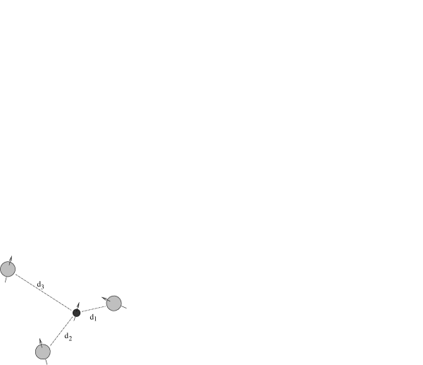
FIG. 1.: Three nuclear spins interacting with an electron spin. The distances $d_{1},d_{2},d_{3}$ determine the interaction strengths $c_{1},c_{2},c_{3}$.

Abstractly speaking, we have a composed system with Hilbert space

$\displaystyle{\mathbb{C}}^{2}\otimes{\mathbb{C}}^{N}\,,$

where $N:=2^{n}$, an interaction Hamiltonian

$$H:=\sigma_{x}\otimes S_{x}+\sigma_{y}\otimes S_{y}+\sigma_{z}\otimes S_{z}\,,$$ (2)

where $S_{x},S_{y},S_{z}$ are self-adjoint operators on ${\mathbb{C}}^{N}$. Furthermore we assume that unitary operations $u\otimes{\bf 1}$ on the controller can be implemented arbitrarily fast, i.e., the time required for the measuring process is essentially determined by the interacting between register and probe particle.

In Section II we describe how to measure the observable $f(S_{\alpha})$ if $f$ is an arbitrary two-valued function on the spectrum of $S_{\alpha}$ with $\alpha=x,y,z$.

In Section III we present some examples for joint observables that are simple to measure in our setting. In Section IV we show that usual two qubit gates can be implemented efficiently if the strength of the interaction between different qubits and the controller can be varied, for instance when the position of the probe particle changes.

II Constructing premeasurements using finite groups

First we describe two simple tricks to convert the interaction

$\displaystyle H:=\sum_{\alpha}\sigma_{\alpha}\otimes S_{\alpha}$

to one of the interactions $\sigma_{\alpha}\otimes S_{\alpha}$ by operating on the controller only: The first method is to intersperse the natural time evolution by fast implementations of $i\sigma_{\alpha}$-rotations on the controller. If the time intervals are made arbitrarily small, the interaction converges to the average Hamiltonian $\sigma_{\alpha}\otimes S_{\alpha}$ (“selective decoupling” techniques, e.g. [6]). Similarly, one can apply a strong magnetic field in $x,y,$ or $z$ direction at the position of the electron spins. To see that a strong field in $z$-direction cancels the $\sigma_{x}$ and $\sigma_{y}$-terms note that the time average of $\exp(i\sigma_{z}Bt)\sigma_{x}\exp(-i\sigma_{z}Bt)$ over the interval $[0,2\pi/B]$ vanishes. Hence the interaction term $\sigma_{x}\otimes S_{x}$ is approximatively cancelled as long as $B\gg\|S_{x}\|$. The same holds for $\sigma_{y}\otimes S_{y}$.

Now we describe how to measure two-valued observables $f(S_{z})$ using the interaction $\sigma_{z}\otimes S_{z}$ if $f(S_{z})$ denotes the operator obtained by application of $f$ in the sense of operator functional calculus. In the following we assume that $S_{z}$ has the eigenvalues $0,1,2,\dots,N-1$. Up to a translation and a time scaling factor, this is the case when $c_{j}=2^{j}$. Note that the translation of the spectrum of $S_{z}$ corresponds to an additional term proportional to $\sigma_{z}\otimes{\bf 1}$ for the probe spin Hamiltonian that is not mentioned explicitly in the following.

The interaction strength $c_{j}$ may be achievable by appropriate distances $d_{j}$ between register spin $j$ and the controller spin.

After the time $t$ the system evolution is given by

$\displaystyle\exp(-it\sigma_{z}\otimes S_{z})\,.$

If the register is in an eigenstate with eigenvalue $j$ the controller evolves according to

$\displaystyle\exp(-ij\sigma_{z}t)\,.$

We describe therefore the total time evolution as

$$({\bf 1},\exp(-i\sigma_{z}t),\exp(-i2\sigma_{z}t),\dots,\exp(-i(N-1)\sigma_{z}t))$$

$$\,\,\,\,\,\,\,\in SU(2)\times SU(2)\times\dots\times SU(2)\,$$

and external unitary operations $u\otimes{\bf 1}$ (where ${\bf 1}$ denotes teh identity) on the controller as

$\displaystyle(u,u,\dots,u)\in SU(2)\times SU(2)\times\dots\times SU(2)\,.$

In both cases, the $j$-th component (note that the counting begins with $0$) of the direct product describes the transformation if eigenvalue $j$ is present.

The evolution caused by the interaction has therefore the abstract form

$\displaystyle(v^{0},v^{1},v^{2},\dots,v^{N-1})\,,$

with $v\in SU(2)$. It is a conditional transformation on the control qubit depending on the state of the register.

Note that every transformation of this form can be implemented: Conjugate the conditional transformation $\exp(-ijt\sigma_{z})$ by an unconditional operation $w$ on the controller and obtain the conditional transformation $w\exp(-ijt\sigma_{z})w^{\dagger}$.

Let $f:\{0,1,2,\dots,N-1\}\rightarrow\{0,1\}$ be an arbitrary function. Then an algorithm for measuring $f(S_{z})$ must have the property that eigenvalues $k,l$ of $S_{z}$ with $f(k)\neq f(l)$ lead to mutual orthogonal controller states and to equal controller states if $f(k)=f(l)$. We can achieve this by a sequence of conditional and unconditional transformations that implements the conditional transformation $u^{f(j)}$ where $u$ is an element of order $2$, i.e., $u\neq{\bf 1}$ and $u^{2}={\bf 1}$. We interpret the transformations as rotations of the controller’s Bloch vector. Then we describe each step of the measurement procedure as an element of

$\displaystyle SO(3)\times SO(3)\times\cdots\times SO(3)\,,$

and the resulting transformation is a rotation by $180$ degree in the $j$-th component of the direct product if and only if $f(j)=1$. One can initialize the controller spin in such a way that its Bloch vector is orthogonal to the rotation axis and achieves that the resulting states of the controller are perfectly distinguishable for different values $f(j)$. This justifies the following definition:

Definition Let $f$ be a function $\{0,1,2,\dots,N-1\}\rightarrow\{0,1\}$. An algorithm for measuring $f$ with $k$ steps is a sequence

$\displaystyle W_{1},W_{2},\dots,W_{k}$

where each $W_{j}$ is of the form $(g,g,\dots,g)$ with $g\in SO(3)$ or $(v^{0},v^{1},\dots,v^{N-1})$ where $v$ is an arbitrary element of $SO(3)$ such that

$\displaystyle W_{k}W_{k-1}\cdots W_{1}=(u^{f(0)},u^{(f(1)},\dots,u^{f(N-1)})$

with $u^{2}={\bf 1}$ and $u\neq{\bf 1}$.

Note that it is irrelevant which element $v$ of order $2$ is chosen since they can be transformed into each other by conjugation with unitaries on the controller. The construction of this kind of measurement procedures has been discussed in [7] by Lie-algebraic methods. Here we are interested in a more explicit design of procedures that does not refer to an infinite number of infinitesimal transformations.

If one restricts the attention to conditional and unconditional transformations in a finite group $G$, the construction of measurement procedures reduces to a word problem in the group $G\times G\times\cdots\times G$ and computer algebra software can be used to solve it. We checked, for instance, that the elements $(g^{0},g^{1},\dots,g^{29})$ and $(g,g,\dots,g)$ with $g$ in the alternating group $A_{5}$ generate the whole group $A_{5}\times A_{5}\times\cdots\times A_{5}$. This means that every function on $30$ equidistant eigenvalues can in principle be measured by $A_{5}$-transformations on the controller. The group $A_{5}$ is the symmetry group of dodecahedron and the icosahedron. If $u\in A_{5}$ has the order $2$ there exists two opposite corners of the dodecahedron or icosahedron that are permuted by $u$. If the probe spin is initialized to one of them one can distinguish the transformations $u$ and ${\bf 1}$ by measuring the resulting state.

Now we show that a measurement process exists for every $N$ and every two-valued function $f$ if one does not restrict the attention to a specific finite group but combine transformations of different finite groups. The following argument shows that it is sufficient to construct measurements for the functions $f_{i}$ with $f_{i}(j):=\delta_{ij}$, where $\delta_{ij}$ denote the Kronecker symbol. An arbitrary function $f$ can be written as

$\displaystyle f:=\oplus_{i\in I}f_{i}\,,$

where $I$ is appropriate subset of $\{0,1,2,\dots,N-1\}$. Since the XOR operation $\oplus$ corresponds to a concatenation of measurement procedures we can restrict our attention to each $f_{i}$.

We construct measurements for all $f_{i}$ by the following recursive scheme: We assume that we have already constructed a procedure for measuring the function $f_{i;k}$ that is defined by $f_{i;k}(j)=1$ if and only if $i=j\,(mod\,\,2^{k})$. Now we describe the measurement for $f_{i;k+1}$. Let the measurement procedure for $f_{i;k}$ implement

$\displaystyle(v^{f_{i;k}(0)},v^{f_{i;k}(1)},\dots,v^{f_{i;k}(N-1)})\,,$

where $v$ is an arbitrary 180 degree rotation.

Let $d$ be a rotation by $2\pi/2^{k+2}$, i.e.,

$\displaystyle d^{2^{k+2}}={\bf 1}\,.$

around an axis orthogonal to the axis of $v$.

Then the recursion runs as follows:

1. Implement the conditional transformation

   
   

   $\displaystyle(d^{0},d^{1},\dots,d^{N-1})\,.$

2. Implement the unconditional transformation

   
   

   $\displaystyle(d^{-i-2^{k}},d^{-i-2^{k}},\dots,d^{-i-2^{k}})\,.$

3. Call the measurement procedure for $f_{i;k}$, i.e., implement

   
   

   $\displaystyle(v^{f_{i;k}(0)},v^{f_{i;k}(1)},\dots,v^{f_{i;k}(N-1)})\,.$

4. Implement the inverse of the transformation in 1, i.e.,

   
   

   $\displaystyle(d^{-0},d^{-1},\dots,d^{-N+1})\,.$

5. Implement the unconditional transformation

   
   

   $\displaystyle(d^{i+2^{k}},d^{i+2^{k}},\dots,d^{i+2^{k}})\,.$

6. Call the measurement procedure for $f_{i;k}$ again.

The resulting transformation implements on the $j$-th component the $SO(3)$-rotation

$$v^{f_{i;k}(j)}d^{i-j+2^{k}}v^{f_{i;k}(j)}d^{j-i-2^{k}}\,.$$ (3)

For every $j\neq i\,(mod\,\,2^{k})$ the rotation is the identity since expression (3) reduces to

$\displaystyle d^{i-j+2^{k}}d^{j-i-2^{k}}={\bf 1}$

due to

$\displaystyle v^{f_{i;k}(j)}={\bf 1}\,.$

Now we distinguish between the two remaining cases

$\displaystyle j=i+(2l+1)\,2^{k}\hbox{ and }j=i+(2l)\,2^{k}\,.$

In the first case expression (3) reduces to

$\displaystyle v\,d^{-2^{k+1}l}\,v\,d^{2^{k+1}l}\,.$

This is the identity since 180 degree rotations around mutual orthogonal axis commute.

For $j=i+(2l)\,2^{k}$ expression (3) is equal to

$\displaystyle v\,d^{2^{k}-2^{k+1}l}\,v\,d^{2^{k+1}l-2^{k}}=v\,d^{2^{k}}\,v\,d^{-2^{k}}$

since $d^{-2^{k+1}l}$ commutes with $v$.

Hence we obtain a rotation by 180 degree since $d^{2^{k}}$ is a 90 degree rotation and the commutator between a 180 degree rotation and a 90 degree rotation around mutual orthogonal axis is a 180 degree rotation. by iteration of this scheme we can implement the function $f_{i;k_{0}}$ for every arbitrary $k_{0}\in{\mathbb{N}}_{0}$. Chosing $k_{0}$ such that $2^{k_{0}}\geq N$ we have a measurement procedure for $f_{i}$.

The number of necessary conditional transformations for measuring $f_{i}$ is then of the order $2^{k_{0}}\,,$ since the measurement of $f_{i;k+1}$ uses the measurement of $f_{i;k}$ twice. Hence the complexity of the measurement is linear in $N$, i.e., exponential in the number of qubits.

We have already mentioned that measurement procedures for two functions $f$ and $g$ can concatenated to measurements for $f\oplus g$. There is also a simple rule to combine two measurements to obtain $f\wedge g$. For doing so we have to achieve that $f$ and $g$ implement $u$ and $v$ respectively with the property that $u$ and $v$ are elements of $S_{4}$ with the property that $w:=u\,v\,u^{-1}\,v^{-1}=u\,v\,u\,v$ is an element of the order $2$. The group $S_{4}$ is the symmetry group of the cube and the octahedron. We can implement the measurement for $g$ followed by the measurement of $f$ and repeat both procedures and we have implemented the transformation

$\displaystyle w^{f(j)\wedge g(j)}\,,$

i.e., a measurement for $f\wedge g$. Note that this kind of “computation on a single qubit” is similar to the so-called ROM-based computation in [8].

III The simplest measurements

The scheme presented in Section II for generic functions $f$ involves a rather large number of transformations. It is straightforward to ask which joint observables are simple to measure. Referring more specificly to our model it would be interesting to know which functions require only rather short sequences of transformations. The following observation is obvious: The basic observable in our model is given by $f_{0;1}(S_{z})$ which was defined as $f_{0;1}(j):=j\,(mod\,2)$ in Section II. This measurement does not require any unitary operations on the control spin, we have only to initialize the probe spin orthogonal to the $z$ axis and wait for the time $t=\pi$. Then the probe spin rotates $180$ degree if the register state is an eigenstate of $S_{z}$ with odd eigenvalue and rotates a multiple of $360^{o}$ if the eigenvalue is even. If all spins are coupled to the probe spin with equal interaction strength, this process measures the parity of the binary word in the register. If the strengths of the couplings are $1,2,4,\dots$ the process measures the observable $\sigma_{z}$ for the spin with the weakest coupling. Single qubit-observables for the other qubits seem to be less simple to measure. Note that the other functions $f_{i;k}$ for $k>1$ (which are relative elementary in our scheme) are not single qubit observables since they refer to the states of at least $k$ qubits.

Now we show how to measure the function $f_{3;2}$ using conditional and unconditional transformations in the dihedral group $D_{8}$, the symmetry group of the octagon. We have checked that all two-valued functions with periodicity $4$ (i.e. $f(j)=f(j+4)$) can be measured by a sequence in

$\displaystyle D_{8}\times\cdots\times D_{8}\,.$

Some of the functions with periodicity $4$ can be implemented by a sequence of $3$ steps and some functions can even be measured by sequences of length $2$. Since it would not give any insights to consider all of them, we will only describe the procedure for $f_{3;2}$. For two qubits with coupling strengths $1$ and $2$, respectively, this is simply the AND function (in Section IV we will use this procedure to implement a controlled-phase-gate on two qubits), in general it measures whether the content of the register is equal to $3$ modulo $4$. Let $u$ be a rotation by $45$ degree around the $z$ axis. Consider $u$ as an element of the dihedral group $D_{8}$. Initialize the probe spin to an arbitrary state in the $(x,y)$-plane. It is sufficient to consider only the eigenvalues $0,1,2\dots,7$ since we use only transformations $w$ with $w^{8}={\bf 1}$ and therefore the probe particle evolves in the same way for $j$ and $j+8$.

Then we use the conditional transformation

$\displaystyle(u^{0},u^{1},\dots,u^{7})\,.$

Fig. 2(a) shows the positions of the resulting states for the eigenvalues $j=0,1,\dots,7$.

FIG. 2.: Positions of the states for the eigenvalues $0,1,\dots,7$ after transformations in the dihedral group $D_{8}$.

Then we implement the conditional transformation

$\displaystyle(v^{0},v^{1},\dots,v^{7})\,,$

where $v$ is a 180 degree rotation in $D_{8}$ around the axis going through point 1 and 5 in Fig. 2(a). The effect is that the state is fixed for all even eigenvalues and mirrored at the $(1,5)$-line for all odd values. The resulting states are shown in Fig. 2(b).

By implementing

$\displaystyle(u^{-0},u^{-1},\dots,u^{-7})$

the state of the probe spin evolves to the positions shown in Fig 2.(c). The states for the eigenvalues group in two classes $\{3,7\}$ and $\{0,1,2,4,5,6\}$ lying on the opposite side of the Bloch sphere. Hence we can distinguish those two classes by measuring the probe spin. The measurement procedure presented here consists of $3$ conditional transformations (“steps”). It would be interesting to know which other observables allow simple measurement procedures. Note that the only function that can be measured in one step is the parity function. This is easy to see: If the conditional transformation

$\displaystyle(u^{0},u^{1},\dots,u^{N-1})$

should only contain rotations by 180 degree, one can only have

$\displaystyle({\bf 1},u,{\bf 1},u,\dots)\,.$

IV Implementing gates on several qubits

The implementation of gates on $n$ spins by addressing only the control spin can directly be performed by measuring procedures. Let $U$ be an $n$-spin transformation that is diagonal in the $\sigma_{z}$-basis. Furthermore assume that $U$ has only two distinct eigenvalues. They can assumed to be $e^{-i\phi},e^{i\phi}$ w.l.o.g. Then we have $U=\exp(i\phi f(S_{z}))$ for some function $f:\{0,1,2,\dots,N-1\}\rightarrow\{-1,1\}$. Apply the following scheme: (1) Initialize the control spin in the state $|0\rangle$ with respect to the $\sigma_{z}$ basis. (2) Perform a measurement of $f$. (3) Implement $\exp(i\phi\sigma_{z})$ on the control spin. (3) Repeat the measurement process (Note that our kind of measurements are their own inverse).

By selecting interactions $\sigma_{x}\otimes S_{x}$ or $\sigma_{y}\otimes S_{y}$ one can similarly obtain unitaries that are diagonal with respect to the $\sigma_{x}$ and $\sigma_{y}$-basis. For each spin $j$ the single qubit transformations

$\displaystyle\exp(i\sigma^{(j)}_{\alpha})$

with $\alpha=x,y,z$ can clearly be implemented by this method. Furthermore the controlled phase gate can be implemented using the measurements process for the AND function of Section III if we neglect a physically irrelevant global phase factor. With $\phi=\pi$ the controlled phase gate is equivalent to a controlled-not by single qubit Hadamard transformation. This shows that the set of gates that can be obtained is universal for quantum computation. If one uses functions $f_{i;k}$ with $2^{k}\geq N$ the process explained above implements a phase shift controlled by the states of all qubits.

Note that the results can in principle be generalized to the case that $S_{x},S_{y},S_{z}$ have non-equidistant spectrum. First we find a suitable rational approximation for the eigenvalues and calculate the least common multiple of the denominators. By rescaling the time by this factor the spectrum can be viewed as a subset of the integers and the algorithm above can be applied.

V Control-spin with different positions

The measurement and control schemes presented above are not efficient at all for controlling and measuring a large number $n$ of qubits since even the computation of simple functions as the monomials $f_{i}$ above requires a number of operations that is linear in $N$ and exponential in $n$ in the case that $S_{z}$ has equidistant eigenvalues. Now we present a model that is only a slight modification with respect to its physical assumptions but changes the computational model significantly: We assume that the controlling electron can be moved and put at different positions (See Fig. 3). Since the coupling strength $c_{j}$ between nucleus $j$ and electron depends on the distance $d_{j}$ between them, the interactions strength is no longer fixed.

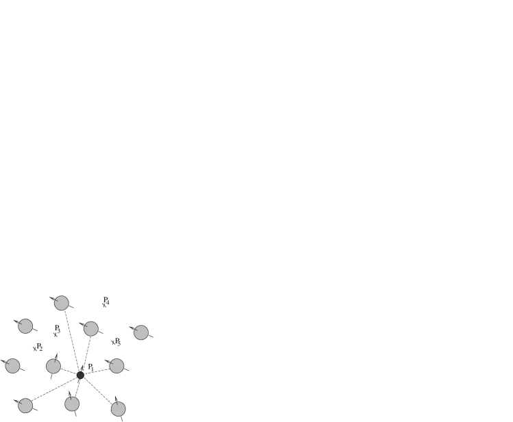
FIG. 3.: The electron can be put at different positions $P_{i}$. This changes the coupling to the different nuclear spins.

Note that the silicon-based quantum computer proposed by Kane [9] also uses the spins of mobile electrons to control nuclear spins. However, this analogy should not be taken to literally since the Kane-proposal does not control several nuclei by the same electron simultaneously.

For a specific position of the electron, we define the “coupling vector” by $C:=(c_{1},c_{2},\dots,c_{n})$ where $c_{j}$ is the strength of the coupling to spin $j$. Now we chose $n$ different points $P_{1},P_{2},\dots,P_{n}$ as possible positions of the electron. In the generic case, we will have that the corresponding coupling vectors $C_{1},\dots,C_{n}$ are linearly independent. Then we can achieve an arbitrary effective coupling vector $C$ as follows: If $C=\sum_{j}d_{j}C_{j}$ we put the electron for the time $t:=|d_{j}|$ at position $j$ and before and after this time interval we implement the transformation $i\sigma_{x}$ on the controller spin if and only if $d_{j}$ is negative. This reverses the sign of the coupling.

This scheme allows to implement usual two-qubit gates efficiently: Set for instance

$\displaystyle C:=(0,0,1,0,\dots,0,2,0,\dots,0)$

with the values $1$ and $2$ at arbitrary positions $i,j$. This allows to measure every boolean function of these two qubits efficiently or to implement arbitrary two qubit gates.

It may also be reasonable to choose

$\displaystyle C:=(0,\dots,0,1,0\dots,0,2,0,\dots,0,4,0,\dots,0)$

in order to control three qubits at once, since the control schemes above are not too complex for $n=3$. In order to compute any function of the Hamming weight of the binary word in the register we choose the effective coupling $C:=(1,1,\dots,1)$. Using the results of Sections II and III we can therefore implement all few qubit operations efficiently.

VI Comparing the model with the quantum gate model

To compare the computational power of our model to the common model with single and two qubit gates as elementary operations we have already mentioned in the last Section that all few qubit gates require complexity $O(n)$ since the electron has to be put at $n$ different positions in the generic case.

Conversely, the operation $(d^{0},d^{1},\dots,d^{N-1})$ which is elementary in our model (provided that there is a position such that the coupling vector is $C=(1,2,2^{2},\dots,2^{n-1})$) requires $n$ controlled phase shift gates each acting on one of the nuclear spins and the electron spin. Note that we do not consider the transformations that can be implemented if one uses the full interaction $H=\sum_{\alpha}\sigma_{\alpha}\otimes S_{\alpha}$. To investigate the computational power of this interaction may be an interesting but difficult task and the simulation of the corresponding time evolution by gate operations is non-trivial.

VII Conclusions

In principle $n$ spins can be controlled by acting on a single control-spin only provided that an appropriate fixed interaction between controller and the $n$ spins is given. Measurements and unitary transformations on the $n$-qubit register can be implemented. For large $n$, this method becomes rather inefficient. However, there are still some interesting joint observables that can be measured efficiently. If all qubits couple with the probe particle via interactions of the same strength, some simple functions of the Hamming weight are easy to obtain. This illustrates in which way certain joint observables can relative directly be measured, even more directly than single qubit observables. Our model shows that single qubit observables are not necessarily the “straightforward elementary observables” of a complex system. Of course one may object that also our model relies on single-qubit measurements on the probe particle. But, if we consider the probe particle as part of the environment and as more directly observable than the system itself, we may maintain our statement that other observables are sometimes more direct than single qubit measurements. However, the objection rather shows the circularity of the deep and interesting question “which quantum observables are most directly accessible?”.

The authors acknowledge discussions with Martin Rötteler. This work is part of the BMBF-project “Informatische Methoden bei der Steuerung komplexer Quantensysteme”.

REFERENCES

- [1] D. DiVincenzo. Two-qubit gates are universal for quantum computation. Phys. Rev A, 51:1015, 1995.
- [2] C. Bennett, J. Cirac, M. Leifer, D. Leung, N. Linden, S. Popescu, and G. Vidal. Optimal simulation of two-qubit Hamiltonians using general local operations. LANL-preprint quant-ph/0107035.
- [3] P. Wocjan, M. Rötteler, D. Janzing, and Th. Beth. Simulating Hamiltonians in quantum networks: Efficient schemes and complexity bounds. Phys. Rev. A. 65:042309, 2002.
- [4] R. Raussendorf and H. Briegel. Quantum computing via measurements only. LANL-preprint quant-ph/0010033.
- [5] D. Leung. Two-qubit projective measurements are universal for quantum computation. LANL-preprint quant-ph/0111122.
- [6] D. W. Leung, I. L. Chuang, Y. Yamaguchi, and Y. Yamamoto. Efficient implementation of coupled logic gates for quantum computing using Hadamard matrices. Phys. Rev. A, 61:042310, 2000.
- [7] D. Janzing, R. Zeier, F. Armknecht, and Th. Beth. Quantum control without access to the controlling interaction. Phys. Rev. A, 65:022104, 2002.
- [8] B. Travaglione, M. Nielsen, H. Wiseman, and A. Ambainis. Rom-based computation: quantum versus classical. LANL-preprint quant-ph/0109016.
- [9] B. Kane. Silicon-based quantum computation. LANL-preprint quant-ph/0003031.