Doppler cooling to the recoil limit using sharp atomic transitions

Abstract

In this paper, we develop an analytical approach to Doppler cooling of atoms by one- or two-photon transitions when the natural width of the excited level is so small that the process leads to a Doppler temperature comparable to the recoil temperature. A “quenching” of the sharp line is introduced in order to allow control of the time scale of the problem. In such limit, the usual Fokker-Planck equation does not correctly describe the cooling process. We propose a generalization of the Fokker-Planck equation and derive a new model which is able to reproduce correctly the numerical results, up to the recoil limit. Two cases of practical interest, one-photon Doppler cooling of strontium and two-photon Doppler cooling of hydrogen are considered.

I Introduction

Laser cooling is one of the greatest achievements of Atomic Physics in the few last decades, having open a thorough new field of applications and led to the first experimental demonstration of the Bose-Einstein condensation in dilute gases ref:FirstBEC . The simplest laser cooling process is the well-known Doppler cooling by a red-detuned standing wave interacting with a two-level atom ref:Houches . A usual way of describing Doppler cooling is to derive a Fokker-Planck equation, leading to a limit “Doppler temperature” given by $T_{D}\equiv\hbar\Gamma/(2k_{B})$, where $\Gamma$ is the width of the transition and $k_{B}$ is the Boltzmann’s constant. The Fokker-Planck equation is valid as long as the mean velocity of the atoms is large compared to the atomic velocity shift due to a fluorescence cycle, which is of the order of the recoil velocity $v_{r}=\hbar k_{0}/M$, where $k_{0}=\omega_{0}/c$ is the wavenumber of the atomic transition and $M$ is the mass of the atom. The Doppler temperature should thus be much larger than the recoil temperature $T_{r}\equiv Mv_{r}^{2}/k_{B}$, which implies

$$\Gamma\gg k_{0}v_{r}\text{ .}$$ (1)

(Note that $k_{0}v_{r}$ is the Doppler effect associated to the recoil velocity). In the present paper, we shall consider two cases in which the inequality (1) is not satisfied, namely the one-photon Doppler cooling of strontium and the two-photon Doppler cooling of hydrogen.

Doppler cooling of strontium has recently been studied by experimental groups, with aims varying from achieving high phase-space densities ref:CoolSr to the study of the coherent backward scattering of light by a disordered cold-atom cloud ref:CohBackS . The idea is to take advantage of the very sharp ($\Gamma\approx 7.5$ kHz), spin-forbidden, line ${}^{1}S_{0}-^{3}P_{1}$ whose theoretical Doppler temperature is comparable to the recoil limit.

Laser cooling of hydrogen atoms, on the other hand, is still a goal to be achieved. Laser cooling of trapped hydrogen atoms was experimentally demonstrated ref:CoolHTrapped , but cooling of free atomic hydrogen is still a defy for experimentalists. The main difficulties are that i) hydrogen forms tightly bonded molecules that should be dissociated before any experiment on atoms can be done, and ii) the optical transitions starting from the fundamental state all fall in the vacuum-ultraviolet (VUV), e.g. at 121 nm for the $1S-2P$ transition. Moreover, although Bose-Einstein condensation of hydrogen was achieved ref:BECH without use of such techniques, laser cooling of hydrogen would certainly improve and simplify the procedure leading to condensation, which can be of considerable practical relevance. Cooling of atomic hydrogen by pulsed two-photon transitions was suggested in 1993 by M. Allegrini and E. Arimondo ref:Maria_Ennio using $\pi$ pulses on the $1S-3S$ transition (wavelength of 200 nm for two-photon transitions). Two-photon transitions present the advantage of dividing the laser frequency by two, which means that the required radiation falls in more favorable wavelength domains. The recent progress on the generation of CW, VUV, laser radiation, in the context of metrological studies of the $1S-2S$ transition ref:1S2S , allows one to realistically envisage the two-photon Doppler cooling of hydrogen in the continuous wave regime on the very sharp $1S-2S$ transition (the lifetime of the $2S$ state is 0.2 s), as we suggested in a previous work ref:DopplerTwoPhoton .

Laser cooling relies on the ability of atoms to perform a great number of fluorescence cycles in which momentum is exchanged with the radiation field in a short time (compared e.g. to the collision time). From this point of view, sharp lines are not suitable for cooling, because the cooling time becomes very long. On the other hand, the Doppler temperature is proportional to the linewidth of the excited level (this result is also valid for two-photon transitions); from this point of view, sharp lines are interesting for cooling. In order to conciliate these antagonistic characteristics of sharp transitions, we proposed in Ref. ref:DopplerTwoPhoton to use the “quenching” of the $2S$ state of hydrogen to control the cycling frequency of the process and we shown that this process allowed to approach the recoil temperature where the Fokker-Planck equation breaks down. In the present work we develop a refined analysis of the Doppler process valid up to the recoil limit both for one- and two- photon Doppler cooling.

II Doppler Cooling with one- and two-photon transitions

Let us consider an atom of mass $M$ and velocity $v$ parallel to the $z$-axis (Fig. 1) interacting with two counterpropagating waves of angular frequency $\omega_{L}$ with $p\omega_{L}=\omega_{0}+\delta$, ($p=1,2$ for resp. one- and two-photon transitions), $\omega_{0}/2\pi=2.5\times 10^{15}$ Hz for H and $4.4\times 10^{14}$ for Sr). We have also $k_{0}\equiv\omega_{0}/c=pk_{L}$. We consider three atomic levels, namely the ground state $|g\rangle$, which is coupled by the radiation, via one- or two-photon transitions, to a sharp level $|s\rangle$ of linewidth $\Gamma_{s}$, and the wide level $|w\rangle$ which is coupled to the sharp level $|s\rangle$ through a quenching process of rate $\Gamma_{q}$ note:quenching and to the ground-level $|g\rangle$ by spontaneous emission (natural linewidth $\Gamma_{w}$). We introduce two simplifying assumptions: i) The wide level $|w\rangle$ can be eliminated adiabatically, so that everything happens as if the sharp level has, due to the quenching process, an effective linewidth

$$\Gamma^{\prime}=\Gamma_{w}\frac{\Gamma_{q}}{\Gamma_{q}+\Gamma_{w}}\equiv g\Gamma_{w}\text{ .}$$ (2)

where $g$ is a controllable quenching ratio. ii) We consider that the sharp and wide levels correspond to the same transition frequency with respect to the ground state. This is a very good approximation for the case of hydrogen, where the quenching couples levels $2S$ and $2P$, that are quasi-degenerated. In the case of the strontium the transition frequencies differ by about 30 %, but this does not affect qualitatively our conclusions. The velocity shift corresponding to spontaneous emission of a photon is thus $v_{r}\equiv\hbar k_{0}/M\approx 3.1$ m/s, or $T_{r}\approx 1.2$ mK for H, and $v_{r}\approx 7$ mm/s and $T_{r}\approx 0.53$ $\mu$K, for Sr.

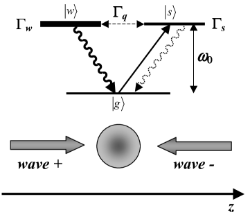
Figure 1: Atomic levels involved in the cooling process. $|s\rangle$ is the sharp level and $|w\rangle$ is the wide level. These levels are coupled by a quenching process of rate $\Gamma_{q}$. Spontaneous emission from the level $|s\rangle$ is very small.

We shall now introduce some specifics of the two-photon Doppler cooling. Four two-photon absorption process are allowed: i) absorption of two photons from the $+z$-propagating wave (named wave “$+$” in what follows), with a rate $\Gamma_{1}$ and corresponding to the a total atomic velocity shift of $+v_{r}$; ii) absorption of two photons from the $-z$-propagating wave (wave “$-$”), with a rate $\Gamma_{-1}$ and atomic velocity shift of $-v_{r}$; iii) the absorption of a photon in the wave “$+$” followed by the absorption of a photon in the wave “$-$”, with no velocity shift and iv) the absorption of a photon in the wave “$-$” followed by the absorption of a photon in the wave “$+$”, with no velocity shift. The two latter process are indistinguishable, and the only relevant transition rate is that obtained by squaring the sum of the amplitudes of these process (called $\Gamma_{0}$). Also, these process are “Doppler-free” (DF) as they are insensitive to the atomic velocity (to the first order in $v/c$) and do not shift the atomic velocity. Thus, they cannot contribute to the cooling process. As atoms excited by the DF process must spontaneously decay to the ground state, this process heats the atoms. In the limit of low velocities, the transition amplitude for each of the four processes is the same. One thus expects the DF transitions to increase the equilibrium temperature by a factor of two, which is verified both numerically and analytically ref:DopplerTwoPhoton . Note that the analysis of the one-photon process can be deduced straightforwardly from the results below by setting the Doppler-free term to zero. The transition rates are given by ref:TwoPhoton :

$$\Gamma_{\pm 1}(V) = \Gamma_{w}\frac{g}{2}\text{ }\frac{\bar{I}^{p}}{(\delta\mp KV)^{2}+g^{2}/4}$$ (3a)

$$\Gamma_{0} = 2\Gamma_{w}g\text{ }\frac{(p-1)\bar{I}^{p}}{\delta^{2}+g^{2}/4}$$ (3b)

where $p=1,2$ corresponds to, resp., one- and two-photon transitions. $\Gamma_{\pm 1}$ describe, respectively, the absorption from the “$+$” and “$-$” waves, and $\Gamma_{0}$ the DF transition rate (note that this terms is equal to zero for one-photon transitions). $\bar{I}\equiv I/I_{s}$ where $I_{s}$ is the saturation intensity, $\delta$ is the detuning divided by $\Gamma_{w}$, $K\equiv k_{0}v_{r}/\Gamma_{w}\approx 0.26$ for H and $K\approx 3.2\times 10^{-4}$ for Sr, and $V\equiv v/v_{r}$. The only qualitative difference between one- and two-photon Doppler cooling, in the present context, is the presence of Doppler-free terms in the latter case. Note that, with the above normalizations, the usual Fokker-Planck approach is expected to break down when $g\leq|\delta|\ll K$.

III Derivation of the generalized Fokker-Planck equation

The rate equations describing the evolution of the velocity distribution $n(V,t)$ and $n^{*}(V,t)$ for, respectively, atoms in the ground and in the excited level are

$${\frac{\partial n(V,t)}{\partial t}}=-\big{[}\Gamma_{-1}(V)+\Gamma_{0}+\Gamma_{1}(V)\big{]}n(V,t)+{\frac{\Gamma^{\prime}}{2}}\big{[}n^{*}(V-1)+n^{*}(V+1)\big{]}$$ (4a)

$${\frac{\partial n^{*}(V,t)}{\partial t}}=\Gamma_{-1}(V-1)n(V-1,t)+\Gamma_{0}n(V,t)+\Gamma_{1}(V+1)n(V+1,t)-\Gamma^{\prime}n^{*}(V,t)\text{ .}$$ (4b)

The deduction of the above equations is quite straightforward (cf. Fig 1). The first term in the right-hand side of Eq. (4a) describes the de-population of the ground-state velocity class $V$ by two-photon transitions, whereas the second term describes the re-population of the same velocity class by spontaneous decay from the excited level. In the same way, the three first terms in the right-hand side of Eq. (4b) describe the re-population of the excited state velocity class $V$ by two-photon transition, and the last term the de-population of this velocity class by spontaneous transitions. For each term, we took into account the velocity shift ($V\rightarrow V\pm 1$) associated with each transition and supposed that spontaneous emission is symmetric under spatial inversion.

For laser intensities below the saturation intensity of the transitions, one can adiabatically eliminate the population of excited level and reduce the Eqs. (4a) and(4b) to one equation describing the evolution of the ground-state population:

$${\frac{dn(V,t)}{dt}} = -\left[\Gamma_{0}+\frac{\Gamma_{-1}(V)}{2}+{\frac{\Gamma_{1}(V)}{2}}\right]n(V,t)+$$ (5)

$${\frac{1}{2}}\Big{\{}\Gamma_{0}\left[n(V-1,t)+n(V+1,t)\right]+\Gamma_{-1}(V-2)n(V-2,t)$$

$$+ \Gamma_{1}(V+2)n(V+2,t)\Big{\}}$$

The set of ordinary differential equations in Eqs. (4a) and (4b) or Eq. (5) has no known analytical solution and must be solved numerically. However, it is possible to develop some analytical approaches following the general idea leading to the Fokker-Planck equation (FPE) for the time-evolution of the velocity distribution (see Refs. ref:DopplerTwoPhoton , ref:FPE ). Taking the continuous limit of Eq. (5) with respect to $V$, we obtain the following “generalized Fokker-Planck equation” (GFPE) note:continuous :

$${\frac{\partial n}{\partial t}=}{\frac{\partial(f_{1}n)}{\partial V}}+{\frac{\partial^{2}\left(f_{2}n\right)}{\partial V^{2}}}$$ (6)

where the functions $f_{1}(V)$ and $f_{2}(V)$ are given by:

$$f_{1}(V) = \Gamma_{-1}(V)-\Gamma_{1}(V)$$ (7a)

$$f_{2}(V) = \Gamma_{-1}(V)+\Gamma_{1}(V)+\frac{\Gamma_{0}}{2}\text{ .}$$ (7b)

In this form, we keep explicitly the $V$-dependent coefficients $f_{1}(V)$ and $f_{2}(V)$. Note however, that this limit implies a smooth variation of the velocity distribution $n(V)$ as well as of the rates $\Gamma_{\pm 1}(V)$ [on a $V$-interval which is $O(1)$]. However, the rates $\Gamma_{\pm 1}(V)$ present sharp peaks at the values $V=\pm\delta/K$ (in the limit $g\rightarrow 0)$ and the GFPE is thus not valid around these values. Note that the standard FPE can be obtained from the above equations in the limit $V\rightarrow 0$:

$$f_{1}(V) = 2V\frac{d\Gamma_{-1}(V)}{dV}$$ (8)

$$f_{2}(V) = 2\Gamma_{-1}(V=0)+\frac{\Gamma_{0}}{2}$$ (9)

where the derivative is evaluated at $V=0$.

Figure 2: Velocity distribution for two-photon Doppler cooling obtained from the GFPE [curve (a)], and FPE [curve (b)] compared to the numerical simulations of Eq. (5) (dashed line). For the sake of comparison all distributions are set to $n(V)=1$ for $V=0$. The distribution temperatures are $T=2.19$ for (a), $T^{\prime}=3.88$ for (b) and $2.16$ for the numerical simulation (temperature in recoil units). Parameters are $g=0.2$ and $K=0.26$.

To our knowledge, the above system has no analytical solution. However, we can focus on their asymptotic steady-state solution. By setting $\partial n{/}\partial t\equiv 0$ in Eq. (6), we straightforwardly obtain:

$$n(V)=\frac{1}{f_{2}(V)}\exp\Big{\{}-\left[\int{\frac{f_{1}(V)}{f_{2}(V)}dV}\right]\Big{\}}$$ (10)

The steady-state distribution is then obtained by integration of Eq. (10) ($f_{1}/f_{2}$ is a ratio of polynomials in $V$ and the integration is obtained by standard methods). One gets:

$$n(V)=\frac{1}{f_{2}(V)}\exp\left[\frac{2\left(\delta^{2}+g^{2}\right)\delta}{K\sqrt{\left(7\delta^{4}+22\delta^{2}g^{2}-g^{4}\right)}}\allowbreak\tan^{-1}\frac{2K^{2}V^{2}-\delta^{2}+3g^{2}}{\sqrt{\left(7\delta^{4}+22\delta^{2}g^{2}-g^{4}\right)}}\right]$$ (11)

[provided $\left(7\delta^{4}+22\delta^{2}g^{2}/4-g^{4}/16\right)>0$ or more simply $|\delta|\gtrsim g/10$. Note that this inequality is fulfilled in most practical situations, since $|\delta|$ must be high enough to allow the system to distinguish the “+” and the “-” cooling beams]. The solution of the FPE, on the other hand, is the gaussian velocity distribution:

$$n^{\prime}(V)=\exp\left[-\frac{1}{2}{\frac{|\delta|K}{\delta^{2}+g^{2}/4}}V^{2}\right]\text{ .}$$ (12)

These velocity distributions are shown in Fig. 2 and compared to the results of a direct numerical simulations of Eq. (5). Eq. (11) compares very well to the numerical solution for $|V|<|\delta|/K\sim 4$ (that is, for the central peak of cold atoms), while the FPE distribution Eq. (12) leads to a broader (hotter) distribution. Both approaches fail to correctly describe the (uninteresting) background of hot atoms.

We can deduce the temperature of the distribution from its the central peak of cold atoms (which typically corresponds to $|V|<|\delta|/K$, that is, to atoms strongly interacting with the radiation) and we neglect the wide background of hot atoms. In this limit, the velocity distribution fits to a gaussian shape $\exp(-V^{2}/2T)$ where $T$ is the temperature in $T_{r}$ units. For the GPFE, we obtain the following analytical expression:

$$T=\frac{(\delta^{2}+g^{2}/4)^{2}}{K\left[-\delta^{3}+3K\delta^{2}-(\delta+K)g^{2}/4\right]}$$ (13)

whereas for the FPE distribution the same approach gives:

$$T^{\prime}=\frac{\delta^{2}+g^{2}/4}{K|\delta|}$$ (14)

Fig. 3 compares both temperatures to the results of numerical simulation. One observes that the values of $T^{\prime}$ increasingly disagrees with the numerical results as one approaches the recoil limit (as expected), and predicts values that are typically too hot by a factor $\simeq 3$ for detunings close the Doppler minimum $|\delta|\simeq g/2$ [obtained from Eq. (14)]. For higher detunings ($|\delta|\gg K$), both the FPE and GFPE approach the same limit $T\simeq|\delta|/K$. Note that for $|\delta|<g/2$ the GPFE approach also breaks down, leading to sub-recoil temperatures. In this case, the peak of cold atoms disappears into the background of hot atoms, it is then hard define a temperature. However, this regime is not of great experimental interest.

Figure 3: Temperature vs. detuning for two-photon cooling. The curve (a) corresponds to the GFPE and the curve (b) to the FPE (both represented by solid lines). The numerical values corresponds to the dashed-dotted line). The agreement is clearly better for the GFPE. Parameters are $g=0.2$ and $K=0.26$.

In the case of the cooling by one-photon transitions, we obtain the velocity distribution simply by setting $\Gamma_{0}=0$ in Eqs. (7b) and (9):

$$n(V) = \allowbreak\frac{\left[(\delta^{2}+g^{2}/4)^{2}+K^{2}V^{2}(\delta^{2}+g^{2}/4)\right]^{\frac{\delta}{K}}}{f_{2}(V)|_{\Gamma_{0}=0}}$$

$$\allowbreak n^{\prime}(V) = \allowbreak\exp\left(-\frac{|\delta|K}{\delta^{2}+g^{2}/4}V^{2}\right)\text{ .}$$ (15)

for the GFPE and FPE cases respectively. One deduces the temperatures of the cold central peak in the same way as above. The result is exactly $T/2$ and $T^{\prime}/2$. The factor two is a consequence of the Doppler-free transitions that increases the equilibrium temperature, as we pointed out in Sec. I and discussed in more detail in Ref. ref:DopplerTwoPhoton .

Figure 4: Velocity distribution for one-photon transitions : GFPE [curve (a)], and FPE [curve (b)] (solid lines) and numerical simulation based on Eq. (5) (dashed line). The temperatures are $T=1.30$ for (a), $T^{\prime}=2.12$ for (b) and $1.4$ for the numerical simulation. Parameters are $K=3\times 10^{-4}$ for strontium, $\delta=4K$ and $g=0.8K$.

Figure 4 shows the distributions compared to the results of a numerical integration of Eq. (5). The GFPE is seen to correctly describe the velocity distribution and the temperature up to the recoil limit. Note that $\delta$ and $g$ must be of the order of $K$ in order to obtain temperatures of the order of the recoil temperature [see Eqs. (13) and (14)].

In the case of hydrogen, a stray effect can show up for the high laser intensities: the photoionization of the excited state, causing a decreasing in the number of cooled atoms. We evaluated the impact of this effect in Ref. ref:DopplerTwoPhoton , and showed that it does not limit the method.

IV Conclusion

In conclusion, we have developed a generalized Fokker-Planck approach allowing to describe Doppler cooling on very sharp lines up to the recoil limit, and showed that the resulting expressions compare very well to the “exact” numerical. This approach can in principle be extended to a more precise description of particular cases.

- (1) M. H. Anderson, J. R. Ensher, M. R. Matthews, C. Wieman, and E. A. Cornell, “Observation of Bose-Einstein condensation in a dilute atomic vapor”, Science 269, 198-201 (2002).
- (2) See for example C. Cohen-Tannoudji in Fundamental systems in quantum optics, École d’été des Houches, Session LIII 1990, J. Dalibard, J. M. Raimond, and J. Zinn-Justin eds., North-Holland, Amsterdam, 1992; W. D. Phillips, ibid., for a very good review of both theoretical and experimental aspects of Doppler cooling.
- (3) K. R. Vogel, T. P. Dinneen, A. Gallagher, and J. L. Hall, Proc. SPIE Int. Soc. Opt. Eng. 3270, 77 (1998); H. Katori, T. Ido, Y. Isoya, M. Kuwata-Gonokami, “Magneto-optical trapping and cooling of Strontium atoms down to the photon recoil temperature”, Phys. Rev. Lett. 82, 1116-1119 (1999).
- (4) Y. Bidel, B. Klappauf, J. C. Bernard, D. Delande, G. Labeyrie, C. Miniatura, D. Wilkowkski, and R. Kaiser, “Coherent light transport in a cold strontium cloud”, Phys. Rev. Lett. 88, 203902 (2002).
- (5) I. D. Setija, H. G. C. Werij, O. J. Luiten, M. W. Reynolds, T. W. Hijmans, and J. T. M. Walraven, “Optical cooling of atomic hydrogen in a magnetic trap”, Phys. Rev. Lett. 70, 2257-2260 (1993).
- (6) T. J. Greytak, D. Kleppner, D. G. Fried, T. C. Killian, L. Willmann, D. Landhuis, and S. C. Moss, “Bose-Einstein condensation in atomic hydrogen”, Physica B 280, 20-26 (2000).
- (7) M. Allegrini and E. Arimondo, “Pulsed laser cooling of hydrogen atoms”, Phys. Lett. 172, 271-276 (1993).
- (8) A. Huber, T. Udem, B. Gross, J. Reichert, M. Kourogi, K. Pachucki, M. Weitz, and T. W. Hänsch, “Hydrogen-deuterium 1S-2S isotope shift and the structure of deuteron”, Phys. Rev. Lett. 80, 468-471 (1998) and references therein.
- (9) V. Zehnlé and J. C. Garreau, “Continuous-wave Doppler cooling of hydrogen atoms with two-photon transitions”, Phys. Rev. A 63, 021402(R) (2001).
- (10) Quenching of the state can be achieved by mixing the and the state. This can be done, e.g., by microwave radiation around 1.04 GHz (the spacing between the two levels) or by a static electric field of a few tenths of volts. For details, see W. E. Lamb and R. C. Retherford, Phys. Rev. 81, 222 (1951); F. Biraben, J. C. Garreau, L. Julien, and M. Allegrini, Rev. Sci. Instrum. 61, 1468 (1990). Quenching in Sr can be done by adding an additional laser radiation coupling the levels () and () at 1.4 m.
- (11) B. Cagnac, G. Grynberg, et F. Biraben, “Spectroscopie d’absorption multiphotonique sans effet Doppler”, J. Phys. Fr. 34, 845-858 (1973).
- (12) J. P. Gordon and A. Ashkin, “Motion of atoms in a radiation trap”, Phys. Rev. A 21, 1606 (1980); see also ref:Houches and refs. therein.
- (13) C. P. Ausschnitt, G. C. Bjorklund, and R. R. Freeman, “Hydrogen plasma diagnosis by resonant multiphoton optogalvanic spectroscopy”, Appl. Phys. Lett. 33, 851-856 (1978).
- (14) The functions , depending on the discrete set of velocities are assumed to vary smoothly; the “continuous limit” consists in replacing, in Eq. (5), the function (for instance) by: , and so on.