Hot entanglement in a simple dynamical model

Abstract

How mixed can one component of a bi-partite system be initially and still become entangled through interaction with a thermalized partner? We address this question here. In particular, we consider the question of how mixed a two-level system and a field mode may be such that free entanglement arises in the course of the time evolution according to a Jaynes-Cummings type interaction. We investigate the situation for which the two-level system is initially in mixed state taken from a one-parameter set, whereas the field has been prepared in an arbitrary thermal state. Depending on the particular choice for the initial state and the initial temperature of the quantised field mode, three cases can be distinguished: (i) free entanglement will be created immediately, (ii) free entanglement will be generated, but only at a later time different from zero, (iii) the partial transpose of the joint state remains positive at all times. It will be demonstrated that increasing the initial temperature of the field mode may cause the joint state to become distillable during the time evolution, in contrast to a non-distillable state at lower initial temperatures. We further assess the generated entanglement quantitatively, by evaluating the logarithmic negativity numerically, and by providing an analytical upper bound.

I Introduction

Interacting quantum systems typically develop correlations in the course of their dynamics, either of classical or of genuinely quantum nature Dynamical ; Purity ; Jens ; Gemmer . If two systems are initially in a pure product state which does not decouple from the interaction Hamiltonian, entanglement will always occur. Depending on the particular type of the interaction and the choice of the initial state, it may well be that the degree of entanglement being generated is very small indeed for a rather long time period Gemmer . Entanglement is nevertheless an unavoidable byproduct of the time evolution. If the joint system is initially in a product state, but with one or both subsystems being mixed, then it is not necessarily clear that entanglement will arise at any point in the dynamics. For finite-dimensional systems it is obvious that whenever the joint system is suitably mixed initially, then the joint state will stay separable at all times. For infinite-dimensional systems, however, a more complex behaviour may be anticipated. Intuitively, one may still expect that if both systems are initially very mixed, then the bi-partite state should not develop entanglement at any time. In the case that one system is in an arbitrarily mixed state and the other is pure, then it is conceivable that entanglement is always generated. This has in fact been demonstrated in the case of a Jaynes-Cummings-type interaction Jaynes ; Jaynes2 ; VogelWelsch of a two-level system coupled to a field mode Purity , and in the Caldeira-Leggett model for quantum Brownian motion, where a single field mode is considered that is linearly coupled to many other field modes initially prepared in some thermal state Jens .

The Jaynes-Cummings model is also particularly suitable to assess the situation when initially both systems are initially in a mixed state. This model describes in the most basic way the interaction between light and matter: it models the dynamics under linear coupling of a two-dimensional system to a near resonant quantised single field mode with a rotating-wave Hamiltonian. The Jaynes-Cummings model can be analytically solved in the sense that the time evolution can be explicitly evaluated for all times. Hence, one may investigate the trade-off between the degree of mixing of the two-level system and the mixing of the field mode.

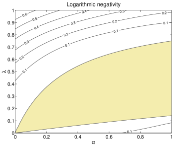
Figure 1: This figure depicts the maximal degree of entanglement that arises in the joint state of a two-level system coupled to a single field mode in the Jaynes-Cummings model. The field mode is initially in a thermal state, the two-level system is prepared in $\lambda|e\rangle\langle e|+(1-\lambda)|g\rangle\langle g|$, $\lambda\in[0,1]$. Zero temperature corresponds to $\alpha=0$, and the limit of infinite temperature is reflected by the limit $\alpha\rightarrow 1$. The degree of entanglement is measured in terms of the logarithmic negativity. The shaded area represents the situation where the log-negativity is zero for all times, meaning that the joint state has a positive partial transpose at all times. In this figure, $\alpha$ is related to the initial inverse temperature $\beta$ of the field mode according to $\alpha=m/(m+1)$, where $m=(\exp(\beta)-1)^{-1}$ is the mean photon number.

In our analysis, we consider the case where the field mode is initially in a thermal state. The set of initial states of the two-level system, from now on labeled as $A$, will be given by

$$\rho_{A}=\lambda|e\rangle\langle e|+(1-\lambda)|g\rangle\langle g|,\,\,\,\lambda\in[0,1],$$ (1)

where $|e\rangle$ and $|g\rangle$ denote the state vectors corresponding to the excited and the ground state, respectively. We will analyse the entanglement properties of the joint system at all times, for all initial temperatures of the field mode and all $\lambda\in[0,1]$. It will turn out that depending on the actual parameters in the model, three regimes can be distinguished: the regime where (free) entanglement is generated immediately, the regime where the joint state will be entangled at some later time $t>0$, and the regime where the joint state has a positive partial transpose for all times. The regime where entanglement will immediately be created is by no means restricted to the case where the two-level system is initially pure. At arbitrarily large temperature of the field mode one may still have a very mixed initial state of the two-level system – yet different from the maximally mixed state – in order to obtain an entangled state for all times.

II Jaynes-Cummings Model for Atom-Field Interaction

The Jaynes Cummings interaction Jaynes ; Jaynes2 of the near resonant interaction with a single mode quantised field with annihilation and creation operators $a$ and $a^{\dagger}$, respectively, can be written as

$$H_{int}=\gamma\left(|e\rangle\langle g|a+|g\rangle\langle e|a^{\dagger}\right).$$ (2)

For simplicity, we set $\hbar=1$ and assume the frequency of the field mode to be unity as well, which does not imply a restriction of generality for our argument. The field mode, associated with the label $F$, is initially prepared in a thermal state with respect to the inverse temperature $\beta>0$, i.e,

$$\rho_{F}=\frac{\exp(-\beta H_{F})}{\text{tr}[\exp(-\beta H_{F})]}=\sum_{n=0}^{\infty}p_{n}|n\rangle\langle n|,$$ (3)

where $H_{F}:=a^{\dagger}a+1/2$ is the Hamiltonian of $F$ and

$$p_{n}:=\frac{m^{n}}{(1+m)^{n+1}}.$$ (4)

$m$ is the mean photon number at the inverse temperature $\beta$, and is given by

$$m:=\left(\exp(\beta)-1\right)^{-1}.$$ (5)

The joint initial state $\rho_{S}\otimes\rho_{F}$ evolves in the interaction picture according to

$$\rho(t)=U(t)(\rho_{S}\otimes\rho_{F})U(t)^{\dagger},\,\,t\geq 0,$$ (6)

where $U(t):=\exp(-iH_{int}t)$. The formal time evolution can be made explicit, as the Jaynes-Cummings model can be analytically solved. The state $\rho(t)$ at a time $t\geq 0$ can be evaluated using the standard techniques to solve the Jaynes Cummings model VogelWelsch . For brevity, we will write $\rho$ instead of $\rho(t)$ from now on. With the above notation, one arrives at

$$\rho=\sum_{n=0}^{\infty}p_{n}\rho_{n},$$ (7)

where

$$\rho_{n}= \lambda \Bigl{[}c_{n}^{2}|e,n\rangle\langle e,n|+s_{n}^{2}|g,n+1\rangle\langle g,n+1|$$

$$+ ic_{n}s_{n}\left(|g,n+1\rangle\langle e,n|-|e,n\rangle\langle g,n+1|\right)$$

$$+(1 - \lambda)\Bigl{[}s_{n-1}^{2}|e,n-1\rangle\langle e,n-1|+c_{n-1}^{2}|g,n\rangle\langle g,n|$$

$$+ ic_{n-1}s_{n-1}\left(|e,n-1\rangle\langle g,n|-|g,n\rangle\langle e,n-1|\right)\Bigr{]},$$

if $n>0$, and

$$\rho_{0} = \lambda\Bigl{[}c_{0}^{2}|e,0\rangle\langle e,0|+s_{0}^{2}|g,1\rangle\langle g,1|$$

$$- ic_{0}s_{0}|e,0\rangle\langle g,1|+ic_{0}s_{0}|g,1\rangle\langle e,0|\Bigr{]}$$

$$+ (1-\lambda)|g,0\rangle\langle g,0|.$$

The symbol

$$\omega_{n}:=2\gamma(n+1)^{1/2}$$ (10)

has been used for the Rabi frequency, and $s_{n}$ and $c_{n}$ are defined as $c_{n}:=\cos(\omega_{n}t/2)$, and $s_{n}:=\sin(\omega_{n}t/2)$ for $n=0,1,2,...$. We will set $\gamma=1$, again for reasons of clarity, which simply corresponds to a rescaling of the units of time.

III Entanglement Properties and Partial Transpose

In order to assess the entanglement properties of the joint state $\rho$ at a later time $t>0$ we investigate the spectrum of the partial transpose $\rho^{\Gamma}$ of $\rho$. This partial transpose takes the form of a direct sum, such that the spectrum of $\rho^{\Gamma}$ can be evaluated from the spectrum of each block. In order to simplify the notation, we set

$$p_{n}=(1-\alpha)\alpha^{n},$$ (11)

with $\alpha\in[0,1)$. The partial transpose is then explicitly given by

$$\rho^{\Gamma} = (1-\alpha)\sum_{n=0}^{\infty}\alpha^{n-1}\Bigl{[}(\alpha c_{n}^{2}\lambda+\alpha^{2}s_{n}^{2}(1-\lambda))|e,n\rangle\langle e,n|$$ (12)

$$+ i(\lambda\alpha-(1-\lambda)\alpha^{2})$$

$$\times c_{n-1}s_{n-1}(|e,n+1\rangle\langle g,n|-|g,n\rangle\langle e,n+1|)$$

$$+ (s_{n-1}^{2}\lambda+(1-\lambda)c_{n-1}^{2}\alpha)|g,n\rangle\langle g,n|\Bigr{]}.$$

From this equation, the spectrum $\sigma(\rho^{\Gamma})$ of $\rho^{\Gamma}$ can be read off: it is given by

$$\sigma(\rho^{\Gamma})=\left\{1-\alpha,\lambda_{0}^{+},\lambda^{-}_{0},\lambda_{1}^{+},\lambda^{-}_{1},...\right\},$$ (13)

where $\lambda_{n}^{+},\lambda^{-}_{n}$, $n=0,1,2,...$, with $\lambda_{n}^{+}\geq\lambda_{n}^{-}$ are the two eigenvalues of the $2\times 2$-matrices

$$M_{n}:=\left(\begin{array}[]{cc}A_{n}&C_{n}\\ C_{n}^{\ast}&B_{n}\\ \end{array}\right),$$ (14)

with entries

$$A_{n} := (1-\alpha)\alpha^{n+1}(c_{n+1}^{2}\lambda+\alpha s_{n+1}^{2}(1-\lambda)),$$ (15)

$$B_{n} := (1-\alpha)\alpha^{n-1}(\alpha c_{n-1}^{2}(1-\lambda)+s_{n-1}^{2}\lambda),$$ (16)

$$C_{n} := i(1-\alpha)\alpha^{n}(\lambda-\alpha(1-\lambda))c_{n}s_{n}$$ (17)

if $n>0$, and

$$A_{0} := (1-\alpha)\alpha(c_{1}^{2}\lambda+\alpha s_{1}^{2}(1-\lambda)),$$ (18)

$$B_{0} := (1-\alpha)(1-\lambda),$$ (19)

$$C_{0} := i(1-\alpha)(\lambda-\alpha(1-\lambda))c_{0}s_{0}.$$ (20)

The remaining task is to identify those values for $\alpha$ and $\lambda$ for which there exists a $t>0$ such that at least one $\lambda_{n}^{-}$ is negative. Due to the form of $M_{n}$ it is obvious that $\lambda_{n}^{+}>0$ for all $n=0,1,2,...$. Hence, it is sufficient to consider the positivity of $\det[M_{n}]$. We first consider the case that $n>0$. The numbers

$$n^{1/2},\,(n+1)^{1/2},\,(n-1)^{1/2}$$ (21)

are not in a rational relationship to each other. Therefore, each contribution to $\text{det}[M_{n}]$ may be individually minimised. Hence, there always exists a time $t>0$ such that $M_{n}$ is given by Eq. (14) with

$$A_{n} = (1-\alpha)\alpha^{n+1}f(\alpha,\lambda),$$ (22)

$$B_{n} = (1-\alpha)\alpha^{n-1}f(\alpha,\lambda),$$ (23)

$$C_{n} = i(1-\alpha)\alpha^{n}(\lambda-\alpha(1-\lambda))/2,$$ (24)

where

$$f(\alpha,\lambda):=\min(\lambda,\alpha(1-\lambda)).$$ (25)

This choice of $t$ corresponds to the sitation where $\text{det}[M_{n}]$ takes its minimal value on the interval $t\in(0,\infty)$. This means that there exists a time $t>0$ with $\det[M_{n}]<0$ if and only if

$$f(\alpha,\lambda)^{2}-(\lambda-\alpha(1-\lambda))^{2}/4<0.$$ (26)

In the case $n=0$, then one arrives with an analogous argument at the statement that there exists a time $t>0$ such that $\det[M_{0}]<0$ if and only if

$$\alpha f(\alpha,\lambda)(1-\lambda)-(\lambda-\alpha(1-\lambda))^{2}/4<0.$$ (27)

Eqs. (26) and (27) provide the desired relationship between $\alpha$ and $\lambda$. Three cases may now be distinguished:

• The values of $\lambda\in[0,1]$ and $\alpha\in[0,1)$ are such that neither Eq. (26) nor Eq. (27) are satisfied. This means that the joint state of the two-level system and the field mode has a positive partial transpose for all times (i.e., it is a PPT state).

• The values of $\lambda$ and $\alpha$ are such that Eq. (27) is satisfied, but Eq. (26) is not satisfied. This means that there exists a time $t>0$ such that the joint state $\rho$ has a non-positive partial transpose (i.e., it is a NPPT state). This time can easily be evaluated: If

  $$\lambda\leq\alpha(1-\lambda),$$ (28)

  then it is given by the time $t>0$ that achieves $c_{0}s_{0}=1/2$ and $c_{1}=1$. If $\lambda>\alpha(1-\lambda)$, then $c_{0}s_{0}=1/2$ and $s_{1}=1$ have to be simultaneously satisfied.

• The values of $\lambda$ and $\alpha$ are such that Eq. (26) is fulfilled. Then, again, the joint state will become a NPPT state. However, now the situation is different compared to case (ii): for any time $t>0$ one can find an $n=1,2,...$ such that $\text{det}[M_{n}]<0$. This means that the joint state $\rho$ becomes an NPPT state instantaneously, or, more precisely, $\rho$ is an NPPT state for all times $t\in(0,\infty)$.

It is important to note that whenever the state is a NPPT state, it is also a free entangled one. This can be seen when considering

$$(1\otimes\pi_{n})\rho(1\otimes\pi_{n})$$ (29)

for $n=1,2,...$, where

$$\pi_{n}:=\sum_{i=n-1}^{n+1}|i\rangle\langle i|.$$ (30)

This is for each $n$ a projection onto a $2\times 3$-dimensional subspace. By investigating the block diagonal structure of $\rho^{\Gamma}$, one finds that the partial transpose of $(1\otimes\pi_{n})\rho(1\otimes\pi_{n})$ has again a direct sum structure. It follows from direct investigation of this projection that $\rho^{\Gamma}$ is non-positive if and only if there exists an $n$ such that $(1\otimes\pi_{n})\rho(1\otimes\pi_{n})$ is non-positive. Hence, whenever one concludes that $\rho$ is NPPT, then it is also free entangled, as for $2\times 3$-systems being NPPT and being distillable are equivalent bound .

The situation that has just been described is depicted in Figs. 1 and 2. In Fig. 1, the white area corresponds to the situation where for some time $t>0$ a free entangled state is reached, which is case (ii). The shaded area is assigned case (i), the PPT case. The lines in Fig. 2 correspond to equality in Eq. (26): then free entanglement is created immediately, as in case (iii).

It is interesting to note that even in the limit $\alpha\rightarrow 1$, which physically is the limit of infinitely large temperature, encounters a PPT state. No matter how large the temperature, there always exists a value $\lambda\in(0,1)$ such that the joint state becomes entangled. The intersection of the parametrised curve of equality in Eq. (26) with $\alpha=1$ associated with ’infinite temperature’ can be easily evaluated. One finds two intersection points at $\lambda=3/4$ and $\lambda=1/4$. The intersection points of the curve of equality in Eq. (27) with $\alpha=1$ are given by $\lambda=1/2-\sqrt{2}/4=0.14645$ and $\lambda=3/4$. That is, whenever $\lambda$ is larger than $3/4$ or smaller than $1/2-\sqrt{2}/4$, then one can be sure that distillable entanglement will be generated. To this extent, both the two-level system and the field mode may therefore be mixed initially. If $\lambda=1/2$, which corresponds to the maximally mixed state for the two-level system, there exists a temperature for which there is no distillable entanglement left. Another interesting situation arises when $\lambda=1/10$ is chosen: Then, at small temperatures, distillable entanglement will be generated. As the temperature increases, that is, with increasing $\alpha$, no free entanglement will occur. But then again, at very large temperatures free entanglement will again arise.

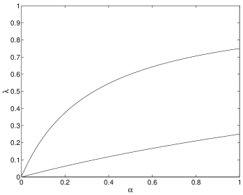
Figure 2: This figure depicts the boundary between the region where free entanglement is created immediately and the region for which there exists a $t>0$ such that the joint state is PPT at time $t$.

From the above considerations, one can also find an upper bound for the distillable entanglement with respect to local operations with classical communication that can maximally be achieved in the course of the time evolution. The log-negativity is such an upper bound for the distillable entanglement. The negativity neg ; vidal of a state $\rho$ is defined as $\|\rho^{\Gamma}\|_{1}-1$, where $\|.\|_{1}$ denotes the trace-norm; it has been shown to be an entanglement monotone vidal ; phd . The log-negativity is nothing but $N(\rho):=\log_{2}\|\rho^{\Gamma}\|_{1}$; it is an easily computable upper bound for the distillable entanglement vidal . Fig. 1 depicts the maximal log-negativity with respect to all times from numerical investigations. Note that around $\lambda=1/10$, the counterintuitive situation occurs that the maximal degree of entanglement that is achieved increases with the initial temperature of the field mode.

An upper bound for the infimum $N(\rho):=\log\|\rho^{\Gamma}\|_{1}$ over all times can be evaluated from the above explicit expression for $\rho^{\Gamma}$. First, note that

$$\|\rho^{\Gamma}\|_{1}=1+2\sum_{n=0}^{\infty}|\lambda_{n}^{-}|.$$ (31)

An upper bound for the log-negativity and therefore for the distillable entanglement can then be evaluated from the extremal sitations in each block of $\rho^{\Gamma}$. One arrives at

$$N(\rho)\leq\log_{2}(1+2\min(0,|\mu^{-}|)+2\min(0,|\nu^{-}|)),$$ (32)

where $\mu^{-}$ and $\nu^{-}$ are the smallest eigenvalues of

$$(1-\alpha)\left(\begin{array}[]{cc}\alpha f(\alpha,\lambda)&(\lambda-\alpha(1-\lambda))/2\\ (\lambda-\alpha(1-\lambda))/2&1-\lambda\end{array}\right)$$ (35)

and

$$\left(\begin{array}[]{cc}\alpha^{2}f(\alpha,\lambda)&\alpha(\lambda-\alpha(1-\lambda))/2\\ \alpha(\lambda-\alpha(1-\lambda))/2&f(\alpha,\lambda)\end{array}\right),$$ (38)

respectively. A particularly simple situation is the case that $\alpha=1$, corresponding to ’infinite temperature’ of the field mode. Then one finds that

$$N(\rho)\leq\left\{\begin{array}[]{ll}\log_{2}(2-4\lambda),&\text{for }\lambda\in[0,1/4],\\ \log_{2}(4\lambda-2),&\text{for }\lambda\in[3/4,1],\\ 0&\text{otherwise.}\end{array}\right.$$ (39)

IV Conclusions and Outlook

In the main part of this paper we have investigated the properties of the dynamically emerging entanglement in the one-photon Jaynes-Cummings model. We have found that three different regimes occur, depending on the actual initial joint product state: there may be free entanglement at all times, and only at a later time. Also, there is the case that the partial transpose of the joint state stays positive at all times, such that the state does not contain distillable entanglement bound . That is, the state is then either separable or bound entangled. One should, however, keep in mind that for bi-partite systems, where at least one part is infinite-dimensional (such as the system considered in this paper), some care is needed when speaking about the separability of a state: the set of non-separable states is then trace-norm dense in the set of all states Halvorson (see also Refs. Pawel ): this means that for any separable state there exists an entangled state arbitrarily close to the original state as measured by the trace-norm, a state that leads consequently to arbitrarily similar probability distributions in quantum hypothesis testing distinguishing the two states. In contrast, there are clearly entangled neighbourhoods of entangled states.

One – possibly not very surprising – principal observation is that the point corresponding to $\lambda=1/2$ and $\alpha=1$ in Fig. 1 is contained in the shaded region. This means that there always exists a temperature such that if both the two-level system $S$ and the field mode $F$ are initially in thermal states corresponding to this temperature, then the composite system will certainly not develop free entanglement. The specific shape of the shaded area in Fig. 1 is clearly a property of the considered one-photon Jaynes-Cummings model. By appropriately choosing the interaction Hamiltonian – for example by introducing a $k$-photon Jaynes-Cummings interaction – one may obviously be in the position to change the shape of this area, and even to make its area very small. If one allows for a time dependence of the interaction, one can also find Hamiltonians such that for all initial temperatures of both parts of a bi-partite system, there will be a time $t>0$ such that the joint system will eventually become free entangled. This leads to the general question whether this connection is unavoidable: there may even be bi-partite infinite-dimensional systems with the property that (i) the thermal states exist for all temperatures for both parts of the system and (ii) with the property that the composite system becomes entangled for all initial temperatures for a fixed time-independent interaction. The existence of such systems may not appear particularly plausible. A complete answer to this question may however lead to a more thorough understanding of the exact link between the initial mixedness of the state of a composite quantum system and the capability of producing entanglement in the course of the time evolution.

V Acknowledgements

This work has been supported by the European Union Networks EQUIP, QUEST, and QUBITS, the EPSRC, the DFG (Schwerpunktprogramm QIV), and the A.-v.-Humboldt-Foundation (Feodor-Lynen-Grants of JE and SS).

References

- (1) K. Zyczkowski, P. Horodecki, M. Horodecki, and R. Horodecki, Phys. Rev. A 65, 012101 (2002); S. Schneider and G.J. Milburn, quant-ph/0112042; H. Mack and M. Freyberger, quant-ph/0206177; M.B. Plenio and S.F. Huelga, Phys. Rev. Lett. 88, 197901 (2002); S. Furuichi, M. Ohya and H. Suyari, Rep. Math. Phys. 44, 81 (1999).
- (2) S. Bose, I. Fuentes-Guridi, P.L. Knight and V. Vedral, Phys. Rev. Lett. 87, 050401 (2001) and erratum, ibid. 87, 279901 (2001).
- (3) J. Eisert and M.B. Plenio, Phys. Rev. Lett. (in print), quant-ph/0111016.
- (4) J. Gemmer and G. Mahler, Eur. Phys. J. D 17, 385 (2001).
- (5) E.T. Jaynes and F.W. Cummings, Proc. IEEE 51, 89 (1963).
- (6) B.W. Shore and P.L. Knight, J. Mod. Opt. 40, 1195 (1993).
- (7) W. Vogel, D.-G. Welsch, and S. Wallentowitz, Quantum Optics, An Introduction (Wiley-VCH, Berlin, 2001).
- (8) M. Horodecki, P. Horodecki, and R. Horodecki, Phys. Rev. Lett. 80, 5239 (1998).
- (9) K. Zyczkowski, P. Horodecki, A. Sanpera, and M. Lewenstein, Phys. Rev. A 58, 883 (1998); J. Eisert and M.B. Plenio, J. Mod. Opt. 46, 145 (1999).
- (10) G. Vidal and R.F. Werner, Phys. Rev. A 65, 032314 (2002).
- (11) J. Eisert, PhD thesis (Potsdam, February 2001).
- (12) R. Clifton, H. Halvorson, and A. Kent, Phys. Rev. A 61, 042101 (2000).
- (13) P. Horodecki, J.I. Cirac, and M. Lewenstein, quant-ph/0103076; J. Eisert, C. Simon, and M.B. Plenio, J. Phys. A 39, 3911 (2002).