Overhead and noise threshold of fault-tolerant quantum error correction

Abstract

Fault tolerant quantum error correction (QEC) networks are studied by a combination of numerical and approximate analytical treatments. The probability of failure of the recovery operation is calculated for a variety of CSS codes, including large block codes and concatenated codes. Recent insights into the syndrome extraction process, which render the whole process more efficient and more noise-tolerant, are incorporated. The average number of recoveries which can be completed without failure is thus estimated as a function of various parameters. The main parameters are the gate ($\gamma$) and memory ($\epsilon$) failure rates, the physical scale-up of the computer size, and the time $t_{m}$ required for measurements and classical processing. The achievable computation size is given as a surface in parameter space. This indicates the noise threshold as well as other information. It is found that concatenated codes based on the $[[23,1,7]]$ Golay code give higher thresholds than those based on the $[[7,1,3]]$ Hamming code under most conditions. The threshold gate noise $\gamma_{0}$ is a function of $\epsilon/\gamma$ and $t_{m}$; example values are $\{\epsilon/\gamma,t_{m},\gamma_{0}\}$ = $\{1,1,10^{-3}\}$, $\{0.01,1,3\times 10^{-3}\}$, $\{1,100,10^{-4}\}$, $\{0.01,100,2\times 10^{-3}\}$, assuming zero cost for information transport. This represents an order of magnitude increase in tolerated memory noise, compared with previous calculations, which is made possible by recent insights into the fault-tolerant QEC process.

The possibility of robust storage and manipulation of quantum information has profound practical and theoretical implications. It would allow highly complex quantum interference and entanglement phenomena, including quantum computing, to be realized in the laboratory, and it also underlies a new and as yet little understood area of physics concerning the thermodynamics of complex entangled quantum systems.

The challenge of achieving precise manipulation of quantum information has inspired much ingenuity, and many established methods of experimental physics, such as adiabatic passage, geometric phases, spin echo and their generalizations can be useful. These provide an improvement in the precision of some driven evolution by a given factor at a cost in speed, for example a slow-down of the evolution by the same factor. Such methods may play a useful role in a quantum computer, but they cannot provide all the stability required, for two reasons. First the slow-down is unacceptable when large quantum algorithms are contemplated, and secondly it is doubtful whether they will in practice achieve the relative precision of order $1/KQ$ which is needed to allow a successful computation involving $Q$ elementary steps on $K$ logical qubits, when $KQ$ reaches values $\gg 10^{6}$ which are needed for computations large enough that a quantum computer could out-perform the best available classical computer.

Quantum error correction (QEC) 95:Shor ; 96:SteaneA ; 96:Calderbank ; 96:SteaneB may allow a precision $\ll 10^{-6}$ per logical operation to be attained in quantum computers. In order for this to be possible, QEC must be applied in a fault-tolerant manner, that is, the QEC process is constructed so that it removes more noise than it generates when it is itself imperfect. The main concepts of fault-tolerance were introduced by Shor 96:Shor , and further insights have been discovered by several authors 96:DiVincenzo ; 98:Preskill ; 98:GottesmanA ; 99:GottesmanB ; 97:KitaevA ; 98:Aharonov ; 98:Knill ; 97:SteaneA ; 97:SteaneC ; 99:SteaneB ; 02:SteaneA . Most of these studies have been concerned with the discovery of methods which achieve fault-tolerance in a quantum computer, and with finding scaling laws which describe how the tolerated noise level varies with the length of the computation. In this paper I address the problem of estimating the amount of noise which can be tolerated, and quantifying the cost of the stability in terms of the required increase in the number of physical qubits in the computer.

Some previous efforts to answer these questions have concentrated on the idea of the threshold. This is the result that arbitrarily long quantum computations can be robust, under various reasonable assumptions, once the noise per quantum gate and per qubit during the duration of a gate is below a threshold value which does not depend on the size $KQ$ of the computation 98:Knill ; 98:Aharonov ; 97:KitaevA ; 97:KitaevB ; Th:Gottesman ; 98:Preskill . Estimates of the value of this threshold have varied between $10^{-6}$ and $10^{-3}$, in the case that gates can act between any pair of qubits in the computer. In view of this wide range, a new calculation of the threshold is valuable, and is one of the aims of this paper. The discussion will include various issues such as the speed of measurements and classical processing, and the best choice of encoding, which have been not been addressed up till now.

However, the threshold result is of limited practical significance, because the encoding it requires (namely multiply concatenated coding) fails to take advantage of a fundamental property of error correction theory, which is the existence of good codes. These have rate $k/n$ and relative distance $d/n$ both bounded from below as the block size $n$ increases; they allow error-free transmission of information at a rate close to the channel capacity. Once the noise is brought moderately below the highest threshold offered by multiply concatenated codes, good encodings (which do not have a threshold result) allow very large quantum algorithms to be stabilized at a much lower cost in scale-up of the physical resources (qubits and operations) of the computer. The only existing estimate 99:SteaneB of what these good codes can achieve used a simple analysis which is only valid in the limit of low noise rate, and which does not take advantage of recent insights into the syndrome extraction process 02:SteaneA . It remains difficult to compare this estimate with the threshold calculations, because each depends on the noise model and the way the noise rate is parameterized, and different authors make different choices. The present paper treats both unconcatenated and concatenated codes together, and so permits a comparison between them.

A central concept which emerges from this uniform treatment is to regard the maximum computation size $KQ$ which can be stabilized as itself a function of various parameters. These parameters divide into two types. The first type quantifies the noise and imprecision which can be tolerated, the second type quantifies the demands on the physical hardware, such as the degree of parallelism and especially the redundancy or scale-up (increase in number of qubits) required. Hence $KQ$ is best understood as a surface, i.e. a function of two main parameters: the tolerated noise level and the physical scale-up. The threshold result is an interesting asymptotic behaviour of this surface in the region of high noise and scale-up, but what we would like to know, and what is also here discussed, is the form of the surface elsewhere in parameter space.

These questions are here addressed by numerical simulations of quantum error correcting networks, and by a detailed approximate analysis.

The paper is laid out as follows. The basic concepts of fault-tolerant quantum computing are briefly sketched in section 1, and the noise model adopted in the rest of the paper is described. Section 2 gives the complete protocol for QEC, explaining various choices about the way the networks are constructed. Section 3 presents the results of numerical simulations of these networks for the case of the $[[7,1,3]]$ Hamming code and the $[[23,1,7]]$ Golay code. Section 4 gives an analysis of the noise and error propagation in the QEC protocol. The numerical results are used to provide values of two fitted parameters, and to confirm the correctness of the general trends predicted by the analysis. The results of the analysis are then presented for 18 different quantum codes, correcting between 1 and 9 errors, and encoding between 1 and 43 qubits per block. Section 5 adapts the analysis to the case of concatenated coding. The results of concatenating once are presented, and the threshold associated with multiple concatenations is calculated. Section 6 then describes and discusses the $KQ$ surface.

Fault-tolerant computation and fault-tolerant data storage are largely similar in that the recovery operations dominate the dynamics. Nevertheless there is a distinction between them. The present treatment is thorough for the case of data storage, and it is argued in section 3 that a judicious placement of logic gates in between recoveries allows the case of fault-tolerant computation to be like data storage with simply some additional noise from those gates. Therefore the present results apply to computation (not just data storage). However a more thorough treatment of the error propagation directly between data blocks is needed in order to clarify this point.

The main results are as follows. First, the threshold for quantum computing using multiply concatenated coding is higher when the code is based on the $[[23,1,7]]$ quantum Golay code rather than the $[[7,1,3]]$ Hamming code. The former also requires a lower scale-up at given $KQ$ than the latter so is advantageous for both reasons. It is found that the time taken to complete measurements and classical processing on qubits is also a significant factor which has mostly been overlooked in previous treatments. When the noise $\epsilon$ per memory qubit per gate time is the same as the noise $\gamma$ associated with a gate, and the measurement of a qubit takes the same time as a quantum gate, the threshold is $\gamma_{0}=\epsilon_{0}\simeq 10^{-3}$. If the measurement takes 100 times longer than a gate, the threshold is $\gamma_{0}=\epsilon_{0}\simeq 10^{-4}$. When the noise per memory qubit per gate time is 100 times smaller than that of a quantum gate, the threshold is $\gamma_{0}=100\epsilon_{0}\simeq 2\times 10^{-3}$ (see figure 7 for more information).

The complete $KQ$ surface, plotted on logarithmic axes, is found to have the shape approximately of a set of inclined planes separated by steep cliffs, revealing quasi-threshold behaviour in scale-up as well as noise (figures 8–10). The jumps in $KQ$ as a function of scale-up occur when new types of encoding become possible. When the noise is an order of magnitude below threshold, and memory is much less noisy than gates, a scale-up of order 10 permits $KQ$ up to $\sim 10^{10}$ by using good codes such as BCH codes. At a scale-up of order 1000, $KQ$ up to $\sim 10^{40}$ is available by using a good code concatenated once with the $[[23,1,7]]$ Golay code. If the memory is as noisy as the gate operations (which could be the case, for example, when information is moved around using swaps between neighbouring bits), a larger scale-up or smaller gate noise is required.

I Basic concepts

A quantum computer stabilized by QEC methods has three stages in its operation. First there is a preparation stage, which places the computer in a close approximation to the state $\left|\right.{0^{(K)}}\left.\right>_{L}$ which is the logical zero state of the $K$ logical qubits of the computer. Then there is a sequence of $Q$ logical operations, interspersed with error correction (also called recovery) of the whole computer. Then the individual physical bits of the computer are measured in the computational basis, and a final error-correction is applied by classical computation to the classical data thus acquired. The overall probability of success is the probability that the classical bit string obtained at the end of this final recovery represents a correct solution to the computational problem being addressed.

For the initial preparation stage, a sufficient approximation to $\left|\right.{0^{(K)}}\left.\right>_{L}$ can be obtained by a fault-tolerant measurement of the logical state of all the logical qubits, combined with an error correction 99:SteaneB , followed by fault-tolerant gates to flip logical bits which were found to be in the logical 1 state.

The final classical correction can be represented in an abstract way as an operation $\cal R$ on the density matrix $\rho(Q)$ of the computer after the $Q$’th computational step. Then a suitable measure of success of stabilization by QEC is the fidelity $F_{Q}\equiv\left<{\psi(Q)}\right|{\cal R}(\rho(Q))\left|{\psi(Q)}\right>$, where $\left|{\psi(Q)}\right>=U_{Q}\left|{0^{(K)}}\right>_{L}$ is the ideal (i.e. noise and imperfection-free) state of the computer after a sequence of $Q$ perfectly-executed elementary steps.

An exact calculation of $F_{Q}$ is extremely difficult, and cannot be attained for a system of even just a few logical bits and operations, owing to the complexities of the encoded states and of the interactions of the physical qubits with each other and the rest of the world. In this paper $F_{Q}$ will be estimated by adopting a very simple noise model and performing a numerical and combinatorial analysis of the QEC networks.

The computer will be encoded using a quantum error correcting code of parameters $[[n,k,d]]$ where $n$ is the number of physical qubits per block, $k$ is the number of logical qubits per block (which N.B. can be greater than 1) and $d$ is the minimum distance of the code. The code is $t$-error correcting where $t=(d-1)/2$. The networks to perform recovery will be built according the recipe put forward in 99:SteaneB ; 02:SteaneA ; 02:SteaneB , which I will outline in section II.

I.1 Noise model

‘Noise’ in the context of QEC is taken to mean any process which causes the state of the physical qubits of the computer to be different from what it should ideally be 96:SteaneB ; 01:SteaneA ; 97:Knill ; 00:KnillB . Thus we include undesired interactions between the qubits, and terms in their internal Hamiltonian and in their coupling to the environment which are known to be present but which cause undesired effects, as well as further terms whose details may be unknown us, all under the umbrella concept of ‘noise’. It is an established feature of QEC that the overall effect of noise can be understood in terms of the set of Pauli operators and the identity acting on the physical qubits. I will write these operators $I,X,Z$ and $Y=XZ$. It is convenient to define the $Y$ operator so that it is real, it then differs from the Pauli operator $\sigma_{y}$ by a factor of $i$ which does not affect the argument.

It is important to distinguish between the processes which cause imperfection in the computer state, which I will call ‘failures’, and the resulting imperfections in the state, which I will call ‘errors’. For example, a single failure of a two-qubit gate can result in two errors, meaning the state after the failure involves errors in two of the physical qubits (that is, a tensor product of Pauli operators on both qubits is required to restore the state). In general after the action of some quantum network, a single failure somewhere in the network can result in multiple errors. The main feature of ‘fault-tolerant’ networks is that a single failure anywhere in the network leads to only one error (or an acceptable number of errors) per encoded block. A set of $m$ single-bit errors on $m$ qubits will also be referred to as an error of weight $m$.

When the noise produces an effect large enough that the computer state cannot be corrected by QEC, the whole quantum computation must be assumed to fail, since it is close to certain that it will not produce a useful result ($F_{Q}\simeq 0$). This situation will be called a crash. QEC and fault-tolerant gate methods allow the crash probability to be much smaller than the failure probability of individual elementary operations on the physical qubits.

The noise model which I will adopt for the purpose of estimating $F_{Q}$ is as follows. At each time step, every freely evolving physical qubit has no change in its state with probability $1-\epsilon$, or undergoes rotation by the operator $X,Y$ or $Z$ with equal probabilities $\epsilon/3$. Such failures are termed ‘memory failures’ and $\epsilon$ is the memory failure probability. Every gate is modeled by a failure followed by a perfect operation of the gate. The failure for a single-qubit gate is the same as a memory failure except that it occurs with probability $\gamma_{1}$. The failure of a two-qubit gate is modeled as a process where with probability $1-\gamma_{2}$ no change takes place before the gate, and with equal probabilities $\gamma_{2}/15$ one of the 15 possible single- or two-qubit failures takes place (these are $IX,IY,IZ$, $XI,XX,XY,XZ$, $YI,YX,YY,YZ$, $ZI,ZX,ZY,ZZ$).

Every preparation of a single physical bit in $\left|{0}\right>$ will be modeled as a perfect preparation follow by a single-bit failure of probability $\gamma_{p}$. Every measurement of a single physical qubit will be modeled as a single-qubit failure of probability $\gamma_{m}$, followed by a perfect measurement. Such a model accounts satisfactorily for the main ways in which measurements can fail, with this exception: a qubit measurement might give a certain eigenvalue $\lambda$ as measured outcome, but the qubit is not projected into the corresponding eigenstate $\left|{\lambda}\right>$. In the present context, however, the latter case is equivalent in its effects to the case which is modeled (i.e. failure followed by perfect measurement), because the measurements are always used to acquire syndrome information. All that matters is that the measured eigenvalue either does or does not correctly indicate the error in the computer: this is accounted for by the model. The case where the syndrome bit was projected onto a state other than $\left|{\lambda}\right>$ does not have any further impact on the computer because we never re-use measured bits without re-preparing them in $\left|{0}\right>$ (a process which has its own failure probability $\gamma_{p}$).

‘Leakage’ failures, which occur when the physical computer moves out of the Hilbert space spanned by the physical qubits, are assumed to be suppressed by techniques such as optical pumping or small leakage measuring networks 98:Preskill and hence converted into failures of the type already considered. The leakage probability is absorbed into the gate and memory failure probabilities.

The model is defined so that qubits participating in a gate in a given time-step undergo gate noise but not memory noise. In other words, the gate noise parameters $\gamma_{i}$ are defined in such a way that they include all the noise acting on the qubits participating in the gate during the time of action of the gate. It is necessary to be explicit about this distinction for the calculation of thresholds in section V.2.

The QEC networks I will analyze are composed only of the single-qubit Hadamard transform and two-qubit controlled-not or controlled-phase gates, and state preparation and measurement of single qubits in the computational basis.

An implicit assumption of this noise model is that failures are uncorrelated and stochastic. The first assumption (uncorrelated failures) can be relaxed without significantly changing the overall results as long as correlated failures have probability sufficiently smaller than uncorrelated ones. In a single time-step, uncorrelated memory failures in $n$ qubits give $m$-bit errors with probability

$$B(n,m,\epsilon)\equiv\frac{n!}{m!(n-m)!}\epsilon^{m}(1-\epsilon)^{n-m}.$$ (1)

If correlated failures (for example due to $m$-body interactions between the physical qubits) have a probability small compared to this then they can be neglected in a calculation of the crash probability without significantly affecting the result. Unwanted systematic effects in a computing device will also cause a finite correlation between the failures in nominally independent gate operations, but if the probability for a weight-$m$ error to be produced by correlated gate failure is small compared to the probability that the same error is produced by uncorrelated gate failures, then it is sufficient to analyze the latter.

Similar statements can be made about non-stochastic contributions to the noise. An example is rotation errors: if a given qubit is erroneously rotated $m$ times by a small angle $\theta$, then if the angles are all in the same direction they add coherently to give a net angle $m\theta$ and error probability $\sim m^{2}\theta^{2}$, whereas if the direction of rotation is random, a random walk is produced resulting in a mean net rotation $\sqrt{m}\theta$ and overall error probability $\sim m\theta^{2}$. The model treated here assumes the latter case; this will cover the main features as long as the coherent contribution gives a net error similar to or less than the incoherent one for each application of the recovery network.

Recently Alicki et al. 01:Alicki have drawn attention to another implicit assumption, namely that the noise is independent of the dynamics of the recovery network, which they show is false for quantum reservoirs with long-range ‘memory’ (such as electromagnetic vacuum). This implies the noise is both correlated and non-stochastic. The argument is subtle and it remains an open question whether the structure of the correlations is of a type which defeats fault-tolerant QEC, or has an influence small compared to the stochastic uncorrelated part which I will estimate here.

II Correction protocol

A fault-tolerant error correction can be accomplished with a variety of choices of exactly how the syndrome extraction network is constructed. Here I will make choices which I have previously argued to be close to optimal, when considerations of noise tolerance and the overall required scale-up are both taken into account.

Transversal operation of a gate means the gate is applied once to each physical qubit in a block, or once to each corresponding pair of physical qubits in a pair of blocks for the case of a 2-qubit gate. Blockwise action of an operator means the operator is applied once to each logical qubit in a block, or once to each corresponding pair of logical qubits in a pair of blocks for the case of a 2-qubit gate.

The QEC code will be a CSS code obtained from a classical code which contains its dual. Such codes have the property that transversal controlled-not and controlled-phase operations act as blockwise controlled-not and controlled-phase operations respectively, and transversal Hadamard acts as blockwise Hadamard 98:GottesmanA ; 99:SteaneB . A further property is useful for constructing fault-tolerant logical operations, though it is not needed for fault-tolerant QEC. This is the property that the underlying classical code is doubly even (i.e. the codewords have weights a multiple of 4) 96:Shor ; 98:GottesmanA ; 99:SteaneB . I will restrict attention here to such codes.

If the algorithm to be accomplished requires $K_{I}$ qubits on an ideal (noise-free) machine, then the real computer has $K$ logical qubits encoded in $K/k$ blocks, each block consisting of $n$ physical qubits, where $K$ is larger than $K_{I}$ by a fixed small amount which can be $<10$. The few extra blocks are necessary as workspace to allow fault-tolerant logical operations on the logical qubits using methods such as teleportation.

For each such ‘data block’ the computer contains in addition $2n_{\rm rep}$ ancilla blocks of $n$ physical qubits each, and $2n_{\rm rep}$ sets of verification bits, each set containing $(n+k)/2$ physical qubits. The total number of physical qubits in the computer is thus

$$N=\left(n+n_{\rm rep}(3n+k)\right)K/k.$$ (2)

$n_{\rm rep}$ is the number of pairs of ancilla blocks per data block which can be prepared in parallel, in order to speed up syndrome extraction; it will have a value typically in the range 1 to 10.

The verification bits are used to verify prepared ancilla states. The stabilizer of the zero state $\left|\right.{0^{(k)}}\left.\right>_{L}$ of a single block (i.e. $k$ logical bits) is generated by a set of $n$ linearly independent operators. This set can be expressed such that it divides into a subset of $(n-k)/2$ which consist of tensor products of $X$ operators, and $(n+k)/2$ which consist of tensor products of $Z$ operators. The ancilla state is verified once against $X$ errors only, by measuring the eigenvalues of the latter subset (the one composed of $Z$ operators) using the verification bits. It is proved in 02:SteaneA that this single verification is sufficient to produce the correct fault-tolerant behaviour when the detailed form of the set of stabilizers is properly chosen.

A single complete recovery consists of $X$-error correction and $Z$-error correction. These two halves of the correction proceed in parallel. While the $X$-error correction machinery is preparing ancilla states, the $Z$-error correction machinery is coupling its ancillas to the data blocks, and vice versa. A single complete $X$-error correction of a single data block proceeds as follows, and the $Z$-error correction is identical except where indicated (for diagrams see 97:SteaneC ; 99:SteaneB ; 02:SteaneB ). Correction of different data blocks proceeds in parallel.

1. Prepare $n_{\rm rep}$ ancilla blocks in $\left|\right.{0^{(n)}}\left.\right>$.

2. Operate a network $G$ in parallel on each of these ancilla blocks. $G$ consists of Hadamards and controlled-not gates, and if perfect would produce the transformation $\left|\right.{0^{(n)}}\left.\right>\rightarrow\left|\right.{0^{(k)}}\left.\right>_{L}$.

3. Using verification bits prepared in $(\left|{0}\right>+\left|{1}\right>)/\sqrt{2}$, verify the ancilla blocks by operating a network $V$ consisting of controlled-phase gates between each ancilla block and its verification bits, followed by Hadamard transformation of the verification bits and their measurement in the computational basis.

4. Ancilla blocks which pass the verification (i.e. all verification bits were found in the state $\left|{0}\right>$ when measured) are deemed ‘good’ and are used in the rest of the protocol. Those that do not are left alone until they are re-prepared at the beginning of the next round of QEC. Let $\alpha$ be the fraction which are good, so that we now have $\alpha n_{\rm rep}$ good ancillas.

5. Couple 1 ‘good’ ancilla to the data block by blockwise controlled-phase (for $X$-error correction) or controlled-not (for $Z$-error correction), with the ancilla acting as control, the data as target. Hadamard transform this ancilla block and then measure each of its physical qubits in the computational basis. Use a classical computer to decode the classical bit string thus obtained, and hence derive the error syndrome 97:SteaneA ; 97:SteaneC .

6. If this syndrome is zero, no further action is taken. The data block rests until recovery has been completed on all the data blocks in the computer whose first syndrome was not zero. Let $\beta$ be the fraction of blocks which give a zero syndrome.

7. (a) Otherwise, couple $r-1$ further good ancillas to the data block by blockwise controlled-phase (controlled-not), for $X$-correction ($Z$-correction), where $r$ is a parameter to be optimized. Hadamard transform and measure these ancillas in parallel, as in step 5.

8. (a) We now have a total of $r$ syndromes extracted for each data block whose first syndrome was non-zero. We accept any group of $r^{\prime}$ syndromes which all agree, where $r^{\prime}$ is a parameter to be optimized. When a syndrome is accepted, the data block is corrected accordingly by application of one or more $X$ gates (or $Z$ gates). If no acceptable syndrome is found, no further action is taken, so the data block goes uncorrected for $X$ errors ($Z$ errors) in this round of QEC.

Steps 7(a) and 8(a) will be modified below, but to understand the modification it helps to begin with the statements as given.

The syndrome repetition factors $r$ and $r^{\prime}\leq r$ will be chosen so as to maximize the probability of success. Increasing $r^{\prime}$ reduces the probability of accepting a wrong syndrome, but increasing $r$ increases the noise accumulating in the data block. The $\alpha n_{\rm rep}-1$ good ancillas per data block which were not used in step 5 are sufficient to allow $r\leq r_{\rm max}=1+(\alpha n_{\rm rep}-1)/(1-\beta).$

In the protocol described we have $\alpha n_{\rm rep}$ good ancillas per data block during each round of QEC, and we require on average $\beta+r(1-\beta)$ for one correction. Hence we have enough ancillas to complete $\alpha n_{\rm rep}/({\beta+r(1-\beta)})$ independent corrections almost in parallel. The sequential part is the gates which couple data and ancilla. Increasing $n_{\rm rep}$ reduces the time during which the data is left alone between corrections, so is valuable when the memory noise accumulating directly in the data contributes a significant part of the total data errors. However, much of the error in the data arises by propagation from the ancillas, or from the gates coupling data and ancillas, and these contributions are unaffected by $n_{\rm rep}$.

We will mostly be interested in the case of large quantum algorithms, for which the failure rates must be small so $\alpha$ and $\beta$ are close to 1, and the number of corrections in parallel is close to $n_{\rm rep}$. The exception is when a concatenated code is being used, with error rates close to the threshold. In this case $\alpha$ and $\beta$ can be of order $0.5$ for the innermost levels of the concatenated coding hierarchy, therefore $n_{\rm rep}$ must be increased to allow sufficient ancillas for rapid correction.

The protocol can be refined primarily in two ways. First, one can operate a different and possibly more sophisticated scheme to prepare and verify ancillas in step 3, and secondly one can adopt a more sophisticated response to the syndrome information in steps 7 and 8.

For example, in step 3 one could verify the ancilla twice and accept if it passed at least once, or one could prepare two ancillas and then compare them by a transversal controlled-not followed by measurement of one. The former case requires more time, which can be compensated by an increase in $n_{\rm rep}$, and the second case requires more ancillas. However, any attempt to improve the ancilla preparation can only result in a modest reduction of the crash probability (at given noise rate) because the gates connecting ancilla and data cause much of the noise in the data, and these cannot be avoided. This is discussed after equations (10), (11) below.

An example of a more sophisticated procedure in step (8) is to extract more syndromes immediately if insufficient syndromes agree. In his calculation, Zalka 99:Zalka employed refinements of this kind. However, such a response is only valuable if it can be made quickly, and this requires fast measurements. It is physically reasonable to suppose that measurement of a qubit may be slow compared to one time step, where a time step is the duration of a two-qubit gate. When measurement is slow it is better to couple syndrome information into ancillas as many times as will be required all at once, and then measure the ancillas in parallel. Therefore if one wishes to extract one further syndrome in step (8) when insufficient syndromes agree, it is advantageous to extract further syndromes as well and one has in the end a protocol close to the one being considered.

There is a modification to steps 7 and 8 which is worth making since it requires only a slight change in the classical part of the processing so has negligible cost. This is to improve the case where no acceptable syndrome was found for a given block. In this case, at the next recovery rather than extracting a further $r$ syndromes, we extract $r^{\prime\prime}\leq r$ where $r^{\prime\prime}$ is another parameter to be optimized, and then make the best use of the $r+r^{\prime\prime}$ syndromes available from the most recent extractions. Typical values for $r^{\prime\prime}$ are in the range $r/2$ to $r$.

1. (b) In the case that at the last recovery, sufficient syndromes were found in agreement for the block to be corrected for the error-type under consideration, proceed as in 7(a). Otherwise, now extract $r^{\prime\prime}-1$ syndromes.

2. (b) In the case that at the last recovery, sufficient syndromes were found in agreement for the block to be corrected for the error-type under consideration, proceed as in 8(a). Otherwise, now examine the $r+r^{\prime\prime}$ most recent syndromes obtained from this and previous recovery attempts. Accept any group of $r^{\prime}$ syndromes which all agree, giving preference to more recently extracted syndromes if there is more than one acceptable group. If there is an acceptable set of syndromes, correct the data block accordingly, otherwise do nothing.

This reduces the noise in the data by making better use of the syndrome information. Further refinements are possible, for example to adjust the case where three successive extractions were necessary, but in any case this is already a small adjustment so there is not much further improvement available.

II.1 Number of recoveries per computational step

It might be thought that when the recovery time $t_{R}\gg 1$, which is typically the case, it would be advantageous to allow many logical gates to operate per recovery, as was argued by Zalka 99:Zalka . However, if the logical gates are not on independent bits, then it is dangerous to allow many of them between recoveries or the error propagation will start to avalanche. Also, it might be argued that sometimes it is only necessary to recover some of the blocks. However, typically the recovery time is long enough that noise accumulating in all blocks is such that they all need correcting. Therefore the choice adopted here is that the whole computer must be recovered after any simple logical gate such as controlled-not or Hadamard is applied. On those occasions in a given algorithm where many logical gates can act simultaneously, then they are implemented in parallel, followed by one complete recovery.

The logical gates are accomplished in a fault-tolerant manner by sequences of appropriately chosen gates and measurements 98:GottesmanA ; 99:SteaneB ; 99:GottesmanB . To quantify the algorithm size $KQ$ precisely, we must be specific about what type of gate we are counting, because some are easier to accomplish than others. For example, a fault-tolerant network for a Toffoli gate may require 8 recoveries, while a controlled-not gate may only require 1 or 2. Since the main quantity to be calculated is the crash probability per recovery of a single block, the “computation size” will be taken to be the number of such recoveries when a code with $k=1$ (one logical bit per block) is used. Codes with $k>1$ require more recoveries because the fault-tolerant constructions are slightly more complicated. It can be shown that for standard logical gates such as controlled-not and Toffoli, networks for $k>1$ exist which involve approximately twice as many recoveries as similar networks for $k=1$, therefore to make a fair comparison it will be assumed here that for a given algorithm, on average twice as many recoveries are needed when $k>1$ than when $k=1$.

II.2 Timing and non-nearest-neighbour coupling

The correction protocol involves networks $G$ and $V$ for preparing and verifying ancillas, measurement of sets of bits, and transversal controlled-gates between ancilla and data blocks. The precise set of operations in $G$ and $V$ is mostly dictated by the structure of the code, with some moderate room for flexibility in the time ordering of gates and in which set of linearly independent parity checks is chosen. The total time taken by the operations, by contrast, and hence the memory noise, is dictated not only by the logic of the network, but also by the physical capabilities of the computing device. It will be assumed here that the computing device is capable of all the parallelism which is logically available in the QEC protocol. Parallel operation of two or more gates is logically available when the gates commute, so that their effect is the same when they are applied all at once or sequentially. For example, the assumption implies that a transversal gate operation takes a single time-step, and that parallel operation is physically available for sets of gates within the $G$ and $V$ networks, which is useful for speeding up the ancilla preparation.

The $G$ and $V$ networks are related to the generator matrix and parity check matrix of the classical code $C$ whose codewords $u$ give the state

$$\left|{0^{(k)}}\right>_{L}=\sum_{u\in C}\left|{u}\right>.$$ (3)

Let $H$ be the check matrix of $C$, then the parallelism available in the $G$ and $V$ networks was shown in 02:SteaneA to allow the controlled-gates in these networks to be completed in $w$ and $w+1$ time steps respectively, where $w$ is the maximum weight of a column or row of the matrix $A$ given by $H=(I\,A)$ where $I$ is the $(n+k)/2\times(n+k)/2$ identity matrix. A further time interval is required for the Hadamard operations and single-bit measurements and state preparations.

Consider the case that 2-bit gates such as controlled-not are only available in the physical computer between neighbouring physical bits. In this case we have to allow some time, and associated noise, for the transport of the physical qubit information from one place to another in the computer. A reasonable rough model of this is to suppose that the speed and precision of a gate between qubits initially separated by distance $s$ scales as $1+s/D$, where the 1 accounts for the cost of the nearest-neighbour gate, and $s/D$ accounts for the cost of bringing the bits together from distance $s$. In this model, $D\simeq 1$ is a reasonable estimate for a computer which transports information by repeated swap operations between fixed physical qubits, and $D\gg 1$ describes a computer which can move information around at little cost. In the QEC network, physical gates are mostly between qubits which can be fairly close together, such as within part of one block, so a value $D\sim 100$ is sufficient to allow $D$ to be large compared to the mean distance $\bar{s}$ spanned by 2-qubit gates involved in the QEC network 02:SteaneB . In the estimates to follow, I will make the simplifying assumption of ignoring the cost of the physical separation between physical qubits. The results for the noise tolerance will therefore be valid only when $\bar{s}\ll D$. I can use the results to roughly estimate what will happen for a computer having smaller $D$ by dividing the tolerated error rates by $1+\bar{s}/D$. Calculations of $\bar{s}$ for two quantum error correcting codes are described in 02:SteaneB .

Another timing consideration is involved in the measurements and the classical processing of the syndromes. It is an important assumption that the verification bits and the error syndromes are in fact measured, and not treated by purely unitary networks. This allows a substantial part of the processing of this information to be done classically, which I assume is both fast and precise. The time involved in measuring a physical qubit and completing classical processing on the measured eigenvalue will be assumed to be $t_{m}$ time-steps, where 1 time-step is the time required for a controlled-not (or controlled-phase) operation. Typical values for $t_{m}$ are in the range $1\leq t_{m}\leq 100$, which may be associated mostly with the measurement time, making the assumption that the classical processor has a clock rate much faster than that of the quantum processor.

III Numerical calculations

The effects of noise and error propagation in the protocol described in section II were numerically calculated. It is possible to do this in an efficient way because it is sufficient to keep track of the propagation of the errors, rather than the evolution of the complete computer state.

The C++ program keeps an array of $2n+(n+k)/2$ binary digits representing $X$ errors in the physical qubits of one data block and one ancilla with its verification bits, and a similar array representing $Z$ errors. Failures are generated randomly in every gate and time-step, according to the model described in section I.1, by adding 1 to members of the $X$ and/or $Z$ error arrays at the locations of those qubits experiencing an $X$ and/or $Z$ failure respectively. The ancilla bits are re-used for the repeated ancilla preparations and for the $X$ and $Z$ syndrome extraction, but memory noise is added to the data block appropriate to the amount of time passing when $2n_{\rm rep}$ ancillas are available in parallel.

The action of each quantum gate in the networks is modeled by first producing random failure, using the model described in section I.1, and then accounting for error propagation. The error propagation part is as follows: a Hadamard gate on a single qubit swaps the $X$ and $Z$ error values for that qubit; a controlled-not gate adds the $X$ error of the control bit to the target bit, and the $Z$ error of the target bit to the control bit; a controlled-phase gate adds the $X$ error value of the control bit to the $Z$ error value of the target bit, and the $X$ error value of the target bit to the $Z$ error value of the control bit.

It was found that a good pseudo-random number generator was needed in order to get reliable results at low crash probability. For example the generator ‘ran0’ in Bk:Press was inadequate; ‘ran3’ was used instead.

The network of gates is obtained directly from the check and generator matrices of the relevant classical codes, see appendix for details. The gate failures were added at the locations in space and time of the relevant gates. The memory failures were not modeled exactly in the right way however. To save program time, during the $G$ and $V$ networks, rather than adding memory failures only to those bits not involved in a gate at a given time, memory failures were distributed randomly amongst all the bits, with probabilities set so that the mean number of failures was correct. This change is not likely to affect the precision of the final result, which in any case can only be compared to physical examples in an approximate way owing to the simple noise model.

The noise caused by logical operations on the data was partially modeled by adding a further gate failure to each qubit in the data between each round of QEC. This completely accounts for single-block gates but not the error propagation between data blocks caused by logic gates between data blocks. However, at any stage typically only a few logical qubits are involved in 2-bit gates, and these can be timed so as to keep error propagation to a minimum, as follows. If a controlled-phase logic gate is to be implemented, it should be placed just after $X$ error correction on both blocks involved, since at this stage in their evolution the blocks temporarily have a minimal number of $X$ errors, and only this type of error is propagated (into $Z$ on the other block) by the gate. Similarly, if a controlled-not gate is to be implemented, it should be placed just after the control bits have had $X$ error correction, and the target bits $Z$ error correction. The cost of this is that sometimes one or a few blocks have to wait a little longer before being corrected, so that memory noise occurring directly in the data block accumulates for longer. However, since this noise is not the main source of data errors, the omission of this detail from the numerical simulation is not expected to affect the final result significantly.

A single logical step consists of a single transversal gate acting on the data block, followed by the complete QEC protocol. The program repeats this $Q$ times to represent an algorithm of $Q$ steps. After each step, the $X$ and $Z$ bit-error arrays are examined to see if the accumulated noise represents an uncorrectable error. If an uncorrectable error has occurred, the run is stopped and a record is kept of how many steps were completed successfully. This is repeated a large number (millions) of times and the relative frequencies of success or a crash are used to obtain estimates of the fidelity of a quantum computer stabilized by QEC, see below. This is a type of Monte-Carlo simulation.

The numerical calculations were carried out for two example codes, the $[[7,1,3]]$ single-error correcting code obtained from a classical Hamming code, and the $[[23,1,7]]$ three-error correcting code obtained from a classical Golay code. The classical codes in both these examples are perfect, so their quantum versions perform especially well.

In order to interpret the $X$ and $Z$ bit-error arrays to discover whether they represent an uncorrectable error, it is necessary to recall the properties of quantum codes. The combination of the $X$ and $Z$ errors represents an error operator $E$ which has acted on the data qubits. However, the weight of $E$ does not in itself determine whether $E$ is correctable. For example, if $E$ is in the stabilizer then it constitutes no error at all. It is necessary to determine rather whether $E\left|{\psi}\right>_{L}$ would be decoded to $\left|{\psi}\right>_{L}$ by a perfect recovery of the computer. To do this I calculate the syndromes $HE_{X}$ and $HE_{Z}$ where $E_{X}$ and $E_{Z}$ are the bit-strings representing the $X$ and $Z$ parts of $E$ respectively, and $H$ is the parity check matrix of the classical code $C$ (equation (3)). Each syndrome has a coset leader, which is the minimal weight error vector which can cause that syndrome. If the weight of the coset leader for either syndrome is greater than the number of errors correctable by the quantum code, then an uncorrectable error has occurred.

The success and crash frequencies provided by the program are interpreted as follows. Let $n_{f}(Q)$ and $n_{s}(Q)$ be the number of runs in which the quantum computer crashed at step $Q$, and the number of runs in which the computer remained successful at step $Q$, respectively. The probability that the computer crashes during step $Q$, given that it has not crashed in steps $1$ to $Q-1$, is then

$$p(Q)=\frac{n_{f}(Q)}{n_{s}(Q)+n_{f}(Q)}$$ (4)

With stochastic noise, this probability is expected to be independent of $Q$ once initial transient effects have died away, and this was found to be the case. The transient behaviour was found to last a few logical steps, with the general form $p(Q)\simeq\bar{p}(1-(5/4)\exp(-Q/2))$ for $Q\geq 1$ where $\bar{p}$ is the average $p(Q)$ for large $Q$. Hence it was sufficient to continue each run to 10 logical steps, and take $\bar{p}\simeq(p(7)+p(8)+p(9)+p(10))/4$. For each case, the simulation was repeated until $n_{f}(Q=10)$ reached 100, so the statistical uncertainty in $\bar{p}$ is expected to be approximately 5%. The random part of the variation in $\bar{p}$ which is visible in figures 1–3 is consistent with this expectation. For $Q>10$, the value of $F_{Q}$ can be estimated as

$$F_{Q}\simeq(1-\bar{p})^{Q}.$$ (5)

The estimation method to be presented in section IV was used to predict the best choice of parameters $r,r^{\prime},r^{\prime\prime}$ in the last two steps of the protocol, and the choice was confirmed by repeated runs of the Monte-Carlo calculations. One expects $r^{\prime}>1$ to be necessary so that the probability of accepting a wrong syndrome is not linear in the noise rates. If was found that for the $[[7,1,3]]$ code, $r^{\prime}=2$ was optimal, and very similar results were found for $r=2$ or 3, $r^{\prime\prime}=1$ or 2. For the $[[23,1,7]]$ code, $r=4,\;r^{\prime}=r^{\prime\prime}=3$ gave the best results for low noise rates, and $r=3,\;r^{\prime}=r^{\prime\prime}=2$ for high noise rates.

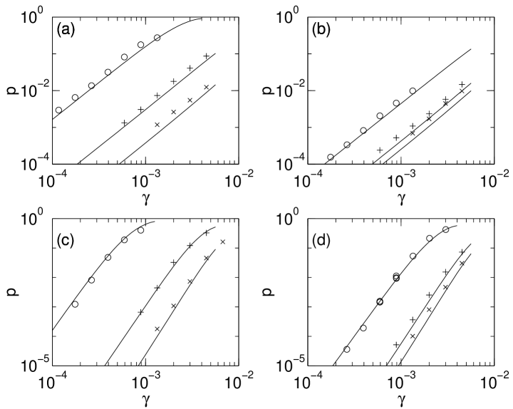
Figure 1: Results of numerical calculations of $\bar{p}$ (symbols) compared with the analytical estimate (curves), at $\alpha n_{\rm rep}=\beta+r(1-\beta)$. The symbols indicate $\epsilon=\gamma$ ($\circ$), $\epsilon=\gamma/10$ ($+$), $\epsilon=\gamma/100$ ($\times$). The calculation used $r=r^{\prime}=r^{\prime\prime}=2$ for the $[[7,1,3]]$ code; $r=4$, $r^{\prime}=r^{\prime\prime}=3$ for the $[[23,1,7]]$ code. (a): $[[7,1,3]]$, $t_{m}=25$; (b): $[[7,1,3]]$, $t_{m}=1$; (c): $[[23,1,7]]$, $t_{m}=25$; (d): $[[23,1,7]]$, $t_{m}=1$.

Figure 2: As figure 1, but for higher $n_{\rm rep}$, here $\alpha n_{\rm rep}=10(\beta+r(1-\beta))$.

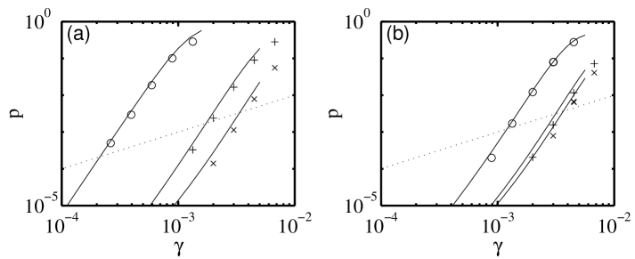
Figure 3: As figure 2, but with reduced $r$ parameters, $r=3,\;r^{\prime}=r^{\prime\prime}=2$ for the $[[23,1,7]]$ code. The dotted lines show the ‘break-even’ condition $\bar{p}=\gamma$ to facilitate a rough estimate of the noise threshold from these results.

Figures 1–3 show example results of these calculations. In each case the points indicate the results of the numerical calculations and the lines show the prediction of the model to be described in section IV. The parameters associated with the choice of code are listed in table 1 of appendix A. The noise parameters were chosen to be $\gamma_{2}=\gamma_{1}=\gamma_{m}=\gamma_{p}\equiv\gamma$, and results for three values of $\epsilon/\gamma$ are shown. Changing $\gamma_{1}$ and/or $\gamma_{m}$ by an order of magnitude while leaving $\gamma_{2}$ fixed does not have a large effect on the results, because the networks are dominated by the 2-qubit gates. The value of $n_{\rm rep}$ can be freely chosen, producing one route for the trade-off between scale-up and noise-tolerance. $n_{\rm rep}$ is accounted for in the numerical calculations simply by adjusting the amount of memory noise in the data bits occurring during each round of QEC. It was convenient to treat the case that $n_{\rm rep}$ varies so that the number of parallel corrections is the same for all values of $\gamma$ and $\epsilon$ in a given set of calculations.

The results in fig. 1 are for $\alpha n_{\rm rep}/(\beta+r(1-\beta))=1$ (i.e. $n_{\rm rep}\simeq 1$) and those in fig. 2 are for $\alpha n_{\rm rep}/(\beta+r(1-\beta))=10$ (i.e. $n_{\rm rep}\simeq 10$). Fig. 3 shows the effect of reducing $r$: this is expected to make matters worse at very low $\gamma$, but better at higher $\gamma$. Comparison of figure 3 with figure 2 shows that a well-chosen reduction in $r$ makes possible a useful increase in the noise threshold (see section V.2).

The comparison between the numerical results in figures 1–3 and the analytical prediction will be discussed in section IV.2 after the analytical estimation method is described.

IV Estimate of crash probability

The numerical method permits the crash probability to be calculated for small codes and high noise rate. A quantum computer performing a large computation will require lower noise rate and larger codes which are able to correct more errors. The Monte-Carlo simulation is too slow to be useful it that regime. In this section I present a general analysis of the QEC protocol which permits an estimate of the crash probability to be made for any code and noise rate. The analysis will also be useful in order to understand the best strategy for code concatenation, to be considered in section V.2.

The main route by which the quantum computer crashes is that too many errors accumulate in the data block between one round of correction and the next. These errors are either caused directly there by noise in the data qubits and the gates which act on them, or they are the result of error propagation from the noisy ancillas. The fault-tolerant design of the QEC network ensures that each failure can only cause one error in any given data block, and more generally each set of $m$ failures can only cause total error of weight $m$ in a data block. Let $g$ be the number of independent gate failure locations which can result in 1 error in the data block, and $s$ be the number of independent memory failure locations which can result in 1 error in the data block, during a single recovery. The probability that an unspecified error of weight $m$ appears in the data is given to good approximation by

$$B^{\prime}(g,s,m,\gamma,\epsilon)\equiv\sum_{j=0}^{m}B(g,j,\gamma)B(s,m-j,\epsilon)$$ (6)

where $B$ is the binomial function defined in equation (1). The sum gives the probability of no gate failures and $m$ memory failures, plus the probability of 1 gate failure and $m-1$ memory failures, and so on up to $m$ gate failures and no memory failures. It involves a slight miss-counting since sometimes different failures have the same effect, so some sets of $m$ failures produce an error of weight $<m$. However, this miss-counting is not expected to give the main limitation on the accuracy of the whole calculation, for the networks under consideration.

An error is uncorrectable if it has a weight larger than $t$. In the limit of small $\gamma$, $\epsilon$, the expression $\bar{p}\simeq 2B^{\prime}(g,s,t+1,2\gamma/3,2\epsilon/3)$ is a rough estimate for the crash probability per block per recovery, and hence it is only necessary to estimate $g$ and $s$ for the QEC network in order to roughly estimate $\bar{p}$ for a given code. The factors of $2/3$ account for the fact that of all the errors affecting any given qubit, on average $2/3$ require $X$-correction and $2/3$ require $Z$-correction. This is true for errors of any weight because they are caused by uncorrelated failures. For example, of the 9 possible 2-qubit errors, 2 require $X$-correction of the 1st qubit alone, 2 of the 2nd qubit alone, and 4 of both qubits: these numbers are correctly given by the model as $9\times(2/3)\times(1-2/3)$ (twice) and $9\times(2/3)\times 2/3$. The overall factor 2 in $\bar{p}$ is because both the $X$ error and the $Z$ error must be correctable.

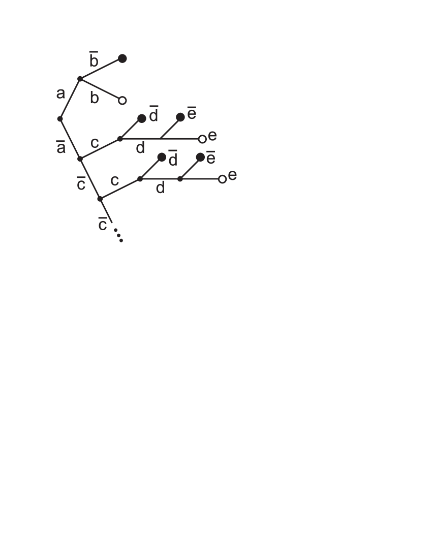
Figure 4: Probability tree to aid the calculation of $\bar{p}$. The branches are labeled as follows. a: First syndrome extracted is zero, b: the single syndrome extraction left a correctable error, c: $r^{\prime}$ of the most recently extracted syndromes are found to agree, d: the accepted syndrome is right, e: the multiple syndrome extraction left a correctable error. The crash probability is the sum of the probabilities of the branches terminated by filled circles.

For a more precise estimate of $\bar{p}$, the protocol must be analyzed more fully. A more complete analysis is indicated in figure 4, which gives a probability tree for the full protocol. I assume the quantum computer crashes not only when an uncorrectable error occurs, but also when a sufficiently bad syndrome is accepted (the latter is discussed further in appendix B). I take into account the fact that the values of $g$ and $s$ will depend on how many syndromes have been extracted before an acceptable one is found allowing a correction to take place. I will use the word recovery to mean one attempt to get a consistent syndrome for each type of error (which will involve either $1$ or $r$ or $r^{\prime\prime}$ syndrome extractions for each type of error) followed by the corrections which take place if sufficient agreement among syndromes is found in step 8 of the protocol. The word correction will now refer to the last stage of recovery only. Thus for any given data block sometimes several recoveries have to take place before a correction can be applied.

Consider the recovery of a single data block. I will consider just the $X$-errors in the data block, and the $X$-syndrome, bearing in mind that $X$ errors in the data are produced partly by the network which extracts $Z$-syndromes. The complete crash probability of the computer per recovery per data block is assumed to be twice the crash probability associated with the $X$-error recovery of this single block.

Let $P_{Z\rm a}$ be the probability a verified ancilla, i.e. one that was deemed ‘good’ in steps 3 and 4 of the protocol, has one or more $Z$-errors, so that it will produce an incorrect syndrome for the data block.

$$P_{Z\rm a} \simeq \sum_{j=1}^{n}B^{\prime}\left(\frac{1}{2}N_{GV}+n(1+\gamma_{1}/\gamma_{2}+\gamma_{m}/\gamma_{2}),\;\frac{1}{2}N_{h}+t_{m}n,\;j,\;\frac{2}{3}\gamma_{2},\;\frac{2}{3}\epsilon\right)$$ (7)

$$\simeq \frac{1}{3}\gamma_{2}N_{GV}+\frac{2}{3}\left(\gamma_{2}+\gamma_{1}+\gamma_{m}\right)n+\frac{1}{3}\epsilon N_{h}+\frac{2}{3}\epsilon t_{m}n$$ (8)

where $N_{GV}=2N_{A}+(n+k)/2$ is the total number of gates in the combined $G$ and $V$ networks; it is dominated by the $2N_{A}$ term, where $N_{A}$ is the number of 1’s in the $A$ part of the check matrix $H=(I\,A)$ from which both the $G$ and the $V$ networks are obtained; $N_{h}$ is the number of ‘holes’ in the $G$ and $V$ networks, that is, the number of locations in space and time where a qubit is resting and so experiences memory- but not gate-failure:

$$N_{h} = \left\{wn-2N_{A}+3(n-k)/2\right\}$$

$$\mbox{}+\left\{w\left(n+(n+k)/2\right)-2N_{A}+(n-k)/2\right\}$$

The parameter $w$ was discussed after equation (3); the first line is the number of holes in $G$, the second is the number of holes in $V$.

The factors of $2/3$ and $1/2$ in (8) account for the fact that of all the failures occurring, some cause purely $X$ error in the ancilla which does not cause a wrong syndrome, and most of those that cause $Y$ error result in the ancilla failing the verification, so they do not affect ‘good’ ancillas. The terms involving $\gamma_{1}$ and $\gamma_{m}$ are the contributions from failure of the final Hadamard gates and measurements of the ancilla bits. The further term involving $\gamma_{2}$ is from the controlled gates connecting ancilla to data. Failures of the preparation of ancilla bits in $\left|{0}\right>$ do not contribute to $P_{Z\rm a}$ because $\left|{0}\right>$ is an eigenstate of $Z$. The term involving $t_{m}$ is the contribution from memory failure in the ancilla during the time taken for the verification bits to be measured. (Equation (8) is discussed further in appendix B).

The fraction $\alpha$ defined in step 4 of the protocol is given approximately by

$$\alpha\simeq 1-\frac{2}{3}\left(N_{GV}\gamma_{2}+n\gamma_{p}+N_{h}\epsilon\right).$$ (9)

This is one minus the probability that a failure of type $X$ or $Y$ occurs in the $G$ and $V$ networks, since almost all such failures are detected by the verification.

In what follows, I will be calculating probabilities for $X$ errors to be present in the data block when the $X$-syndrome extraction is performed. These $X$ errors have three origins: the gates associated with the logical operation which evolves the logical quantum computation; the ${}^{C}\!Z$ gates which link an ancilla or ancillas to the data block for $X$-syndrome extraction; and the network for the preceding $Z$-syndrome extraction (including error propagation from those ancillas to the data). In a given recovery either 1 or $r$ or $r^{\prime\prime}$ extractions of each type take place, I calculate the probability of each case and deduce the average effect.

Let $g(r_{X},r_{Z})$ be the number of independent gate failures resulting in an $X$ error in the data when a network accomplishing $r_{X}$ $X$-syndrome extractions and $r_{Z}$ $Z$-syndrome extractions is applied. For the same network, let $s(r_{Z})$ be the number of independent space-time locations of memory failures that result in an $X$ error in the data. $s$ does not depend on $r_{X}$ because propagation from the ancillas used for $X$-syndrome extraction produces $Z$ not $X$ errors in the data.

$$\!\!\!\!\!\!\!\!g(r_{X},r_{Z}) \simeq n(1+r_{X}+(1+\mu t)r_{Z}),$$ (10)

$$s(r_{Z}) \simeq n\left(t_{R}+(\nu t+t_{m})r_{Z}\right),$$ (11)

$$\mbox{where}\;\,t_{R} = (2w+1+2t_{m})\frac{\beta+r(1-\beta)}{\alpha n_{\rm rep}}$$ (12)

and $\mu,\nu$ are constants of order 1 to be determined. The fraction $\beta$ was defined in step 6 of the protocol; $t_{R}$ is the time the data bits ‘rest’ between successive recoveries. The estimates of $g$ and $s$ are the most important to get right, because they lead directly to the probability of uncorrectable errors in the data. In the expression (10) for $g$ the first term is caused by the $n$ elementary gates of a single transversally-applied logic gate which may be present between recoveries in the protocol adopted, the second term accounts for failure of the transversal ${}^{C}\!\!Z$ gates connecting ancillas to the data block to extract $X$-syndromes, and the third term the effect of the $Z$-syndrome extractions. In the last case only, error propagation from the ancilla causes $X$ errors in the data. These errors are caused by failure of the last gates in the $V$ network; their effect is estimated by the term $n\mu tr_{Z}$ in $g$ by the following reasoning. The last gate of $V$ to act on each ancilla bit can leave an $X$-error there which is not detected by the verification bits; most pairs of gate failures from the last or the penultimate set to act on each ancilla bit can leave undetected single or double $X$-errors; triples of gate failures from a still larger set can go undetected, and so on. This means that the distribution of undetected ancilla errors caused by failures in $V$ is not binomial: the number of failure locations which can contribute to an order-$m$ failure is not independent of $m$ but increases approximately linearly with $m$. I can nevertheless use a binomial as an approximation to the true distribution, as long as I make the approximation sufficiently accurate for the most important probability I wish to calculate, which is the probability of uncorrectable error in the data block. For a $t$-error correcting code, this is the probability of order-$(t+1)$ failures. The term $n\mu tr_{Z}$ in $g$, and a similar term in $s$, approximately counts the relevant locations, where the constants $\mu$ and $\nu$ were found by fitting the theory to the numerical results, see figures 1–3 and section IV.2. The values $\mu\simeq 0.35$, $\nu\simeq 1$ were found to give the best fit.

Note that, as remarked in section II, improving the fidelity of the ancillas can only slightly reduce $g$ because it can only reduce $\mu$ to a minimum of 0, and it can only allow a slight reduction in the syndrome repetition parameters $r,r^{\prime},r^{\prime\prime}$.

The first term in the expression for $s$ (equation (11)) accounts for the memory noise in the data block during the time $t_{R}$ which has to pass between successive recoveries. $t_{R}$ can be reduced by increasing $n_{\rm rep}$. If $t_{R}<(t_{m}+r)$ then the syndromes for the next recovery are extracted before the measurement of the current ones can be completed. However, as long as the classical processing of the syndrome information takes this into account, it need not be a problem. The rest of (11) accounts for the memory noise in the ancillas which is not detected by the verification and can propagate to the data. The term $n\nu tr_{Z}$ follows from an argument similar to the one just given for $g$, and the other term accounts for the period of waiting while the verification bits are measured, which has to be completed before the ancilla is coupled to the data (if it is found to be good).

The fraction $\beta$ defined in step 6 of the protocol is equal to the probability $P_{0}$ that the data block has no $X$ errors, multiplied by the probability $(1-P_{Z\rm a})$ that this fact is indicated correctly by the first syndrome extracted. I estimate

$$P_{0} \simeq \beta B^{\prime}\!\left(g(1,1),s(1),0,\frac{2}{3}\gamma_{2},\frac{2}{3}\epsilon\right)$$ (13)

$$+ \!\!\!(1-\beta)B^{\prime}\!\left(g(1,r),s(r),0,\frac{2}{3}\gamma_{2},\frac{2}{3}\epsilon\right)\!,$$

$$\beta = P_{0}(1-P_{Z\rm a}).$$ (14)

The reasoning is that since the last $X$-error correction, the $Z$-syndrome extraction network required either 1 or $r$ syndromes, with probabilities $\beta$ and $(1-\beta)$ respectively, and only a single $X$-syndrome extraction has been undertaken so far because we are at step 6 of the protocol. Note that for equation (13) I have assumed that whenever the first syndrome is non-zero, $r$ are extracted, which results in a slight underestimate of $\beta$ since in fact sometimes $r^{\prime\prime}<r$ are extracted. Also, I ignore the variation of $\beta$ from one recovery to another. The imprecision associated with these simplifications is small compared to the imprecision of the whole calculation. Equations (11)–(14) are circular, but enable $\beta$ to be found by iteration, starting from a value in the range $0<\beta<1$.

Let ${\cal P}_{1}(r_{X})$ be the probability that an uncorrectable error accumulates in the data when $r_{X}$ $X$-syndromes, and either 1 or $r$ $Z$-syndromes, are extracted in a single recovery attempt. I take an error of any weight above $t$ to be uncorrectable, so

$${\cal P}_{1}(r_{X}) \simeq \!\!\sum_{m=t+1}^{n}\beta B^{\prime}\!\left(g(r_{X},1),s(1),m,\frac{2}{3}\gamma_{2},\frac{2}{3}\epsilon\right)$$

$$\!\!\!\!\!+(1-\beta)B^{\prime}\!\left(g(r_{X},r),s(r),m,\frac{2}{3}\gamma_{2},\frac{2}{3}\epsilon\right)\!.$$ (15)

It is found that for a viable computer (i.e. $\bar{p}\ll 1$) this is the largest contribution to the overall crash probability $\bar{p}$.

Let $P_{\rm agree}(j)$ be the probability that in step 8 of the protocol sufficient syndromes are found to agree for correction to be completed, where $j$ is the number of successive recoveries since the last time an $X$-syndrome was accepted for the block in question, so that an $X$-error correction took place. I argue that agreement is found whenever $r^{\prime}$ or more good syndromes have been prepared without $Z$ error, hence

$$P_{\rm agree}(1)\simeq\sum_{m=r^{\prime}}^{r}B\left(r,m,1-P_{Z\rm a}\right)$$ (16)

and, using the protocol as in steps 7(b), 8(b),

$$P_{\rm agree}(j>1)\simeq\sum_{m=r^{\prime}}^{r+r^{\prime\prime}}B\left(r+r^{\prime\prime},m,1-P_{Z\rm a}\right).$$ (17)

(This estimate breaks down at $r^{\prime\prime}=0$ but I always require $r^{\prime\prime}\geq 1$.)

Let $P_{\rm ws}$ be the probability of a crash caused by a group of $r^{\prime}$ syndromes conspiring to agree on a syndrome, even though they are all wrong, which would result in the wrong ‘correction’ being made to the data. I estimate

$$P_{\rm ws}\simeq N_{GV}(\gamma_{2}/3)^{r^{\prime}}+N_{h}(\epsilon/3)^{r^{\prime}}.$$ (18)

$P_{\rm ws}$ is much smaller than $(P_{Z\rm a})^{r^{\prime}}$ because to accept a wrong syndrome it is necessary that the same error in the ancilla happens in $r^{\prime}$ independent ancilla preparations. Any single $Z$-failure will cause the ancilla to be in a state of non-zero syndrome. Since there are many more possible syndromes than individual failure locations in the ancilla preparation network, it is rare that two different failure locations give rise to the same final error in the ancilla. Therefore the probability of obtaining an ancilla state of the same non-zero syndrome in $r^{\prime}$ independent preparations is, to lowest order in $\gamma,\epsilon$, the probability that the same failure happens in all the preparations. This is approximately $(\gamma/3)^{r^{\prime}}$ multiplied by the number of different gate failure locations, plus a similar term accounting for memory failure. The factors $1/3$ appear because almost all failures which produce $Y$ errors are detected by the verification, so do not affect good ancillas, and those which produce $X$ errors do not produce a wrong syndrome. Note, (18) does not include terms for the noise in the gates connecting ancilla to data, nor the memory noise while the verification bits are measured, nor noise in the ancilla measurement. This is because noise at these locations causes predominantly single-bit errors in the ancilla, and these are almost harmless—see appendix B—the further contribution to $P_{\rm ws}$ is negligible when $(t_{m}\epsilon)^{2}\ll\gamma_{2}$ and $\gamma_{m}^{2}\ll\gamma_{2}$.

It is found that for small codes and/or high noise rate, smaller values of $r,r^{\prime},r^{\prime\prime}$ are better, in order to reduce $\cal P$; for large codes and/or low noise rate, higher values of $r,r^{\prime},r^{\prime\prime}$ are better, in order to reduce $P_{\rm ws}$ and to keep $P_{\rm agree}$ sufficiently large. Once $r^{\prime}$ is large enough, the value of $\bar{p}$ is insensitive to $P_{\rm ws}$ because it is dominated by the other terms.

I can now calculate $\bar{p}$, using the probability tree shown in figure 4 as a guide:

$$\bar{p}(C,\{\gamma_{i}\},\epsilon) \simeq 2\left\{\beta{\cal P}_{1}(1)+(1-\beta)\left[P_{\rm agree}(1)\right.\right.$$

$$\left.\left.\left(P_{\rm ws}+(1-P_{\rm ws}){\cal P}_{1}(r)\right)+S\right]\right\}$$ (19)

where $C$ refers to the set of parameters $\{n,k,t,w,N_{A},r,r^{\prime},r^{\prime\prime},t_{m},n_{\rm rep}\}$ and $\{\gamma_{i}\}=\{\gamma_{1},\gamma_{2},\gamma_{p},\gamma_{m}\}$. $S$ is the sum of the probabilities associated with the lower branches of the tree, when the first recovery attempt gave no consistent syndrome. To calculate these, rather than keeping account of all the possibilities, I use an average for the number of $Z$-syndrome extractions which take place in each recovery. This average is

$$\bar{r}\simeq\beta+(1-\beta)(P_{\rm agree}(1)r+(1-P_{\rm agree}(1))r^{\prime\prime}).$$ (20)

I then have for the probability of uncorrectable $X$-error after a total of $j>1$ recovery attempts since the last correction:

$${\cal P}_{j}\simeq\sum_{m=t+1}^{n}B^{\prime}\left(g(r+(j-1)r^{\prime\prime},j\bar{r}),s(j\bar{r}),m,\frac{2}{3}\gamma_{2},\frac{2}{3}\epsilon\right).$$ (21)

and

$$S\simeq\sum_{j=2}^{\infty}\left\{\prod_{i=1}^{j-1}\left(1-P_{\rm agree}(i)\right)\right\}P_{\rm agree}(j)\left(P_{\rm ws}+(1-P_{\rm ws}){\cal P}_{j}\right)/j.$$ (22)

The final division by $j$ accounts for the fact that I am calculating an average crash probability per attempt at recovery. The logical quantum computation continues whether or not any one recovery attempt gave a consistent syndrome.

IV.1 Illustrative example

To illustrate the main features of the calculation, consider for example the $[[127,43,13]]$ BCH code, for parameter values $\gamma=10^{-4}$, $\epsilon=10^{-6}$, $n_{\rm rep}=2.5$, $t_{m}=25$, and we choose $r=5,\;r^{\prime}=4,\;r^{\prime\prime}=3$. The code has $w=47$, $N_{A}=1802$ (see table 1) giving $N_{GV}=3689$, $N_{h}=8893$. In each time step approximately $N_{A}/w\simeq 38$ gates act in parallel on each ancilla during preparation and verification; the recovery time is $t_{R}=143$ time steps.

These parameter values give $\alpha\simeq 0.74$, $\beta\simeq 0.8$. Suppose the computer consists of 10 blocks. Of the 25 ancillas prepared for $X$-recovery, on average $25\alpha\simeq 18$ are found to pass the verification. When the first syndrome is extracted for each block, $10\beta\simeq 8$ are found to be zero, 2 non-zero. For $r=5$, a further 4 syndromes are extracted from each of the two blocks needing further attention, this uses up the remaining 8 ancillas which passed verification. The ancilla error probability is $P_{Z\rm a}\simeq 0.1$ and the probability a data block has no errors is $P_{0}\simeq 0.9$, therefore the typical situation is that one of the two blocks being recovered is found in fact to be free of errors (its first reported non-zero syndrome was wrong, caused by a $Z$-error in the ancilla preparation) while the other has a correctable error. The probability that 4 of the 5 syndromes agree is $P_{\rm agree}\simeq 0.8$ so the error is usually identified first time, but occasionally this must await the next recovery. In the latter case the subsequent recovery of the block in question has $r+r^{\prime\prime}=8$ syndromes available, the probability that 4 of them are mutually consistent is approximately $0.998$.

The probabilities of uncorrectable error in the data (branches $\bar{\rm b}$ and $\bar{\rm d}$ in fig. 4) are

$${\cal P}_{1}(1) \simeq 3\times 10^{-13}\beta+5\times 10^{-10}(1-\beta)\;\simeq\;3^{-11}$$

$${\cal P}_{1}(r) \simeq 8\times 10^{-12}\beta+2\times 10^{-9}(1-\beta)\;\simeq\;4\times 10^{-10}$$

while the probability of accepting a wrong syndrome is $P_{\rm ws}\simeq 5\times 10^{-15}$. The overall result is $\bar{p}\simeq 3\times 10^{-10}$. It is seen that the main contribution to the crash probability comes from the occasions where repeated syndrome extractions are required for both the $X$ and $Z$ recoveries, leading to too many errors in the data. On these occasions the number of gate and memory failure locations is $g(r,r)=2540$, $s(r)\simeq 39000$ respectively, therefore gate failure dominates when $\epsilon<\gamma/15$.

IV.2 Comparison of analytical estimate and Monte-Carlo simulation

The prediction given by equations (8-22) is shown by the curves in figures 1-3. The main feature of both the numerical results and the analytical estimate is that $\bar{p}$ varies as $(\gamma+\mbox{const.}\epsilon)^{t+1}$ in the limit of small $\gamma$, $\epsilon$. This is seen for example in equation (15), where a useful pair of approximations is

$$B^{\prime}(g,s,m,\gamma,\epsilon) \simeq B\left(g,m,\gamma+s\epsilon/g\right)$$ (23)

$$\simeq \left(\frac{g\gamma+s\epsilon}{m/e}\right)^{m}$$ (24)

The first approximation is quite accurate in the regime under consideration (small $\gamma$, $\epsilon$), while the second gives the right order of magnitude; $e$ is the base of natural logarithms and I used Stirling’s formula to simplify $m!$ (even though $m$ is not large).

The values of the fitted parameters $\mu$ and $\nu$ were adjusted to get the best fit between the curves and the Monte-Carlo ‘data’. This implies that the curves must match the data in at least two places. The fact that the curves also correctly show all the major trends as a function of $\epsilon$, $\gamma$, $n_{\rm rep}$, $t_{m}$ and the code parameters is evidence that the analysis is sufficiently complete to be useful. The analytical estimate predicts that $\bar{p}$ falls slightly faster than $\gamma^{t+1}$ in the region $10^{-4}<\bar{p}<10^{-2}$ because the mean number of syndromes extracted is falling as $\beta$ increases towards 1. The simulations are consistent with this but in the absence of simulated points at $\bar{p}<10^{-4}$ it was not possible to confirm it thoroughly. The Monte-Carlo simulation was too slow to explore the latter region (each point at $\bar{p}\simeq 10^{-4}$ took many days to compute on a modern workstation).

The agreement overall is good. The main (but still modest) discrepancy is that in figures 1 and 2 the analysis underestimates the numerical results, while in figure 3 it overestimates. In other words, the effect of changing the $r$ parameters is greater in the numerical simulation than in the analysis, in the region of large $\gamma$ and small $\epsilon/\gamma$. By adjusting $\mu$ and $\nu$ it was possible to get a better fit either to figures 1 and 2, or to figure 3; the choice shown ($\mu=0.35,\;\nu=1$) represents the best compromise.

There is a small systematic disagreement in gradient for several of the sets of results, especially in figure 1. This would be enough to cause a disagreement in $\bar{p}$ by an order of magnitude if it persisted to lower $\gamma$ values of order $\gamma=10^{-4}$ (where a direct comparison between numerical and analytical results is not available). However, the analytical model always produces the power-law behaviour $\bar{p}\propto\gamma^{t+1}$ at low $\gamma$ (as long as $r^{\prime}\geq t$) so the disagreement in gradient will not persist to low $\gamma$, and in any case when $\bar{p}<10^{-8}$ even an order of magnitude error in $\bar{p}$ will only be a relatively small effect in the results to be obtained from the model in the rest of the paper.

The part of the analysis which can only be confirmed to a limited extent by the simulations is the linear scaling with $t$ of the terms $\mu t$ and $\nu t$ in (10), (11). Simulations of more codes, especially codes correcting more errors, would be necessary to give further information.

IV.3 Performance of a selection of codes

The estimated crash probability (19) was calculated for a variety of codes with scale-up $N/K$ in the range 7 to 400. The gate and measurement noise parameters were set to $\gamma_{1}=\gamma_{2}=\gamma_{m}=\gamma_{p}\equiv\gamma$, and $\bar{p}$ was calculated for several values of $\gamma$ with $\epsilon=\gamma/100$ and with $\epsilon=\gamma/10$, at $t_{m}=25$, $n_{\rm rep}=1$. The values of $r,r^{\prime},r^{\prime\prime}$ were adjusted to minimize $\bar{p}$ for each case. To make a useful comparison, I then consider not $\bar{p}$ directly, but rather the number of qubit-gates $KQ$ which the stabilized computer can achieve, allowing for the fact that codes with $k=1$ allow slightly more efficient fault-tolerant gates than codes with $k>1$, c.f. section II.1. Using the method of ‘propagating the gate through a teleportation’ 99:GottesmanB only approximately twice as many recoveries per gate are needed when $k>1$ than when $k=1$ 99:SteaneB , so $KQ=1/\bar{p}\;(0.5/\bar{p})$ when $k=1$ ($k>1$) respectively. The resulting values of $KQ$ are plotted in figure 5 as a function of the scale-up for the code employed. The codes themselves are identified in table 1 of appendix A.

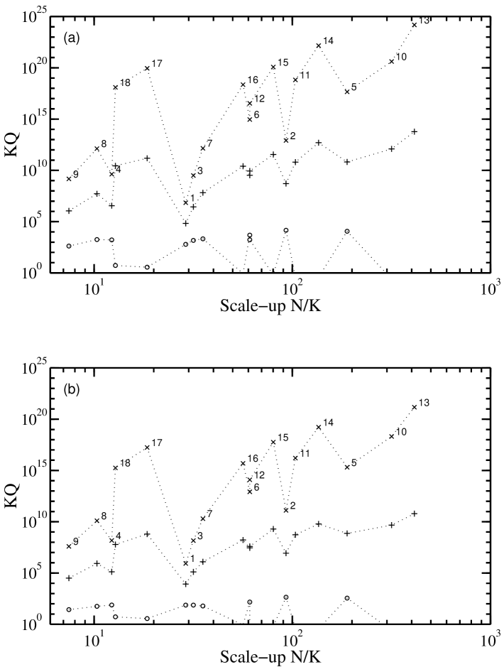
Figure 5: Available $KQ$ for a variety of codes, plotted against the scale-up $N/K$ of each code at $n_{\rm rep}=1,\;t_{m}=25$. (a): $\epsilon=\gamma/100$, (b): $\epsilon=\gamma/10$. The sets of results are at $\gamma=10^{-5}$ ($\times$), $10^{-4}$ ($+$), $10^{-3}$ ($\circ$); each code has a given scale-up, the codes are indicated by an index number placed by each point at $\gamma=10^{-5}$, which refers to the list in table 1. The dotted lines joining the points at given $\gamma$ are to guide the eye.

Clearly at given values of $\gamma,\;\epsilon$ one would choose the code of smallest scale-up which allows a desired $KQ$ to be attained. The main conclusion to be drawn from figure 5 is that for $\gamma\leq 10^{-4}$, the efficient codes such as $[[127,43,13]]$, $[[127,29,15]]$ perform well, but at higher noise level other codes such as those numbered 1 to 9 in table 1 should be adopted, at a cost in scale-up.

V Code concatenation

In order to get still smaller crash probabilities, and hence larger algorithms, we need codes which can correct more errors. Such codes exist, for example a $[[511,241,31]]$ BCH code, but they of necessity involve more parity checks and therefore larger networks to extract syndromes. The increase in $g$, $s$ and $P_{Z\rm a}$ trades off against the increase in $t$, and as a result these codes only become useful at low values of the failure rates, $\gamma<10^{-5}$.

Code concatenation enables this trade-off to be avoided, at the cost of increased scale-up.

V.1 Crash probability of concatenated code

For stabilizing quantum memory, any code $C^{i}=[[n^{i},k^{i},d^{i}]]$ can be concatenated with any other code $C^{o}=[[n^{o},k^{o},d^{o}]]$, but for quantum algorithms the task of constructing logical gates is rendered much more simple if $k^{i}=1$ and both codes are CSS, therefore I restrict attention to this case. With $k^{i}=1$, $n^{i}n^{o}$ physical bits are used to store $k^{o}$ logical bits. $C^{i}$ is called the inner code, and $C^{o}$ the outer code, and their combination is called the supercode. The physical bits will be called ‘level-0’ bits. Consider $n^{o}$ groups containing $n^{i}$ physical qubits each. To build the logical zero state of the concatenated code, first prepare each group of $n^{i}$ level-0 bits in the logical zero of $C^{i}$ (e.g. by using a fault-tolerant measurement). Each such block is then one ‘level-1’ bit. Next use transversal Hadamard and controlled-not operations to evolve the $n^{o}$ level-1 bits into the logical zero state of $C^{o}$. This network may or may not involve a level-1 recovery (i.e. recovery of the level-1 qubits in parallel, using the inner code) before each transversal gate.

A concatenated code can be regarded in two ways. First, it can be regarded as a single CSS code of parameters $[[n^{i}n^{o},k^{o},d]]$ where $d=(d^{i}d^{o}+d^{i}+d^{o}-1)/2$. The methods described in previous sections apply directly, the only change being in the way the classical processor interprets the syndromes. Owing to the code construction, to be uncorrectable an error must be composed of more than $t^{i}=(d^{i}-1)/2$ single-bit errors in each of more than $t^{o}=(d^{o}-1)/2$ sub-blocks. The probability for this is approximately

$$B\left(n^{o},t^{o}+1,B(n^{i},t^{i}+1,p)\right)$$ (25)

where $p$ is the single-physical-bit error probability. The equations (15) and (21) for $\cal P$ have to be adjusted accordingly. This first approach produces useful behaviour when the 7-bit and 23-bit codes are combined once with themselves or each other, but for larger codes the $G$ and $V$ networks become too large to allow recovery unless the noise rates $\gamma$ and $\epsilon$ are very low.

The second way to use a concatenated code is to make more use of its structure, by recovering the encoded level-1 qubits inside the network which prepares level-2 ancillas. For example, if after every gate in the level-2 network, a level-1 recovery is applied to all level-1 qubits, then the overall behaviour is described by the analysis given in section IV, i.e. equations (8) to (22), applied to the blocks of level-1 qubits. The gate and memory failure probabilities $\gamma_{1},\epsilon_{1}$ of the level-1 qubits are estimated as the crash probability per block per recovery associated with the inner code, i.e. $\gamma_{1}=\epsilon_{1}=\bar{p}(C^{i},\gamma,\epsilon)$, and then the crash probability of the supercode is $\bar{p}\simeq\bar{p}(C^{o},\gamma_{1},\epsilon_{1})$.

We can improve matters further by distributing the inner recoveries more intelligently. The main point is that it is better not to recover resting qubits when this will make them more noisy. To do better, after the initial preparation of the level-1 qubits at the beginning of the level-2 $G$ network, a level-1 recovery is applied in parallel to all level-1 qubits, but thereafter recover only non-resting level-1 qubits, just before a gate acts on them, with one exception. The exception is the qubits in the data block, which rest for a long time if $t^{i}_{R}\gg 1$, so these qubits are given level-1 recoveries at the same rate as the qubits in the ancilla. With this method, each level-1 qubit is recovered on average once every $\eta\simeq 1+N^{o}_{h}/2N^{o}_{GV}\simeq 2$ steps of the level-2 network. The effect can be estimated by replacing the term $n^{i}t^{i}_{R}$ in equation (11) by $\eta n^{i}t^{i}_{R}$ in the calculation of $\gamma_{1}=\epsilon_{1}=\bar{p}(C^{i},\gamma,\epsilon)$, and then for the calculation of $\bar{p}=\bar{p}(C^{o},\gamma_{1},\epsilon_{1})$ use the fact that the memory noise in between gates of the outer $G$,$V$ networks has been absorbed into $\gamma_{1}$, therefore set

$$N^{o}_{h}=0,\;\;t^{o}_{m}=1,$$ (26)

and replace $n^{o}t^{o}_{R}$ by $n^{o}t^{o}_{R}/\eta$. This more intelligent placement of inner recoveries was found to reduce $\bar{p}$ for all the cases plotted in the figures.

A small saving on ancilla preparation can be obtained by re-using the $n^{o}$ level-$1$ qubits of any ancilla which failed its level-$2$ verification.

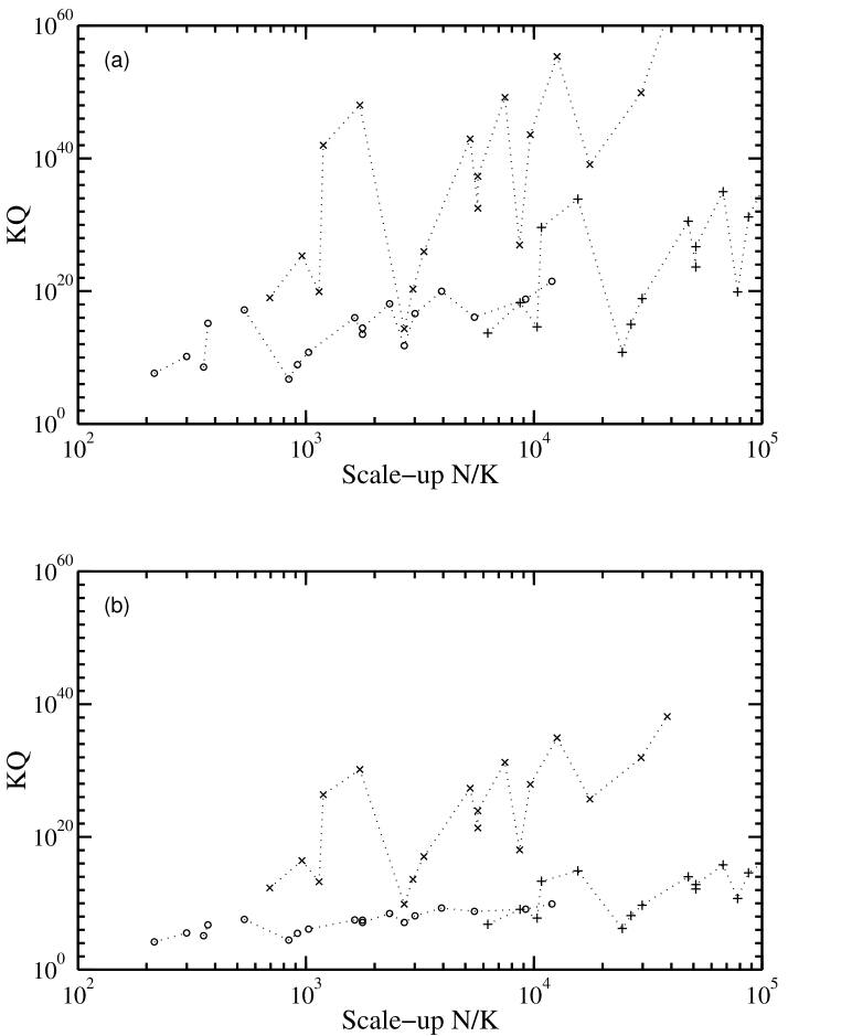
Figure 6: Available $KQ$ verses overall scale-up for codes concatenated with an inner $[[7,1,3]]$ Hamming code ($\circ$) or $[[23,1,7]]$ Golay code ($\times$) or concatenated twice with the Hamming code ($+$). The results are given for the same set of codes as in figure 5 and table 1. The case $\gamma=10^{-4}$, $t_{m}=25$ is shown, for a computer with $n_{\rm rep}=1$ for both inner and outer code. (a): $\epsilon=\gamma/100$, (b): $\epsilon=\gamma/10$.

I show in figure 6 the effect of concatenating the codes of table 1 with the $7$-bit or $23$-bit code once, or with the $7$-bit code twice, estimated by the method just described, at $n_{\rm rep}=1$, $t_{m}=25$. The main conclusion is that the $23$-bit code is a better choice than the $7$-bit code, since for given scale-up it permits the higher $KQ$. It is clear that a great increase in $KQ$ is available from the concatenation of the 23-bit code with another code. In particular, the combination $C^{i}=[[23,1,7]]$, $C^{o}=[[127,29,15]]$ gives a very stable computer for scale-up around 1000.

V.2 Threshold

So far I have calculated the size of computation $KQ$ which can be achieved for a given scale-up and given values of the failure probabilities $\gamma,\epsilon$. Further use of concatenation leads to the ‘threshold result’, which is the result that the situation $\bar{p}\rightarrow 0$ can be obtained for values of $\gamma$, $\epsilon$ below a threshold $\gamma_{0}$, $\epsilon_{0}$ which does not depend on $K$ and $Q$, assuming that the noise per qubit and per gate is independent of the size of the computer and is stochastic and uncorrelated, and sufficient parallel operation is available in the computing device. The threshold result may be proved by analyzing the case of a particular code such as $[[7,1,3]]$, concatenated to arbitrarily many levels. $\bar{p}\rightarrow 0$ is obtained when the crash probability at each of the higher levels is less than that of the level below.

The protocol I have adopted is not guaranteed to be the absolute optimal one, and in particular a protocol which had a higher scale-up and allowed a slightly higher threshold may exist. However, the protocol has been optimized in several ways, such as minimizing the number of gates which connect ancillas to data, and minimizing the time to verify ancillas, therefore it is unlikely that another protocol will offer significant increases in the threshold, under the assumptions which have been made about the noise and the timing. After the first two levels, $\bar{p}$ is $O(\gamma^{(t+1)^{2}})$, i.e. varying quickly with $\gamma$, and therefore the threshold is insensitive to details of the protocol at higher levels.

An estimate of the threshold is immediately available by using the analysis described in section V.1, extended to many levels. I use the analytical estimate $\bar{p}_{L}=\bar{p}(C,\bar{p}_{L-1},\bar{p}_{L-1})$, employing the adjustment given by (26), for the second level, and then higher levels are modeled by taking $t_{m}=1$ without any adjustment to $N_{h}$. The adjustment of $t_{R}^{i}$ by $\eta$ described just before (26) has negligible effect when $n_{\rm rep}$ is large so does not affect the maximum possible threshold.

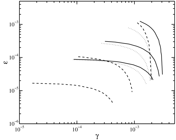
Figure 7: Threshold values $\gamma_{0}$ and $\epsilon_{0}$, for $t_{m}=1$, 25 and 100. Values in the range $0.01\leq\epsilon/\gamma\leq 1$ are plotted. Full curves: concatenated $[[23,1,7]]$, dashed curves: concatenated $[[7,1,3]]$, dotted curves: concatenated $[[47,1,11]]$. The highest value of $t_{m}$ produces the lowest curve of each triplet.

The calculated threshold is shown in figure 7 for the codes $[[7,1,3]]$ Hamming, $[[23,1,7]]$ Golay, and $[[47,1,11]$ quadratic residue, for three values of $t_{m}$ at the innermost level, and for $0.01\leq\epsilon/\gamma\leq 1$. It is seen that if the measurements are fast ($t_{m}=1$), the two smaller codes give a similar threshold, that of the Golay code being somewhat higher. For the more physically realistic case of slow measurements ($t_{m}\gg 1$), the Golay code offers a threshold higher than that of the Hamming code by a factor 2 to 5. The Golay threshold values are in the region of $10^{-3}$ when $t_{m}=1$ or $\epsilon\ll\gamma$, falling to $\sim 10^{-4}$ when $t_{m}\gg 1$ and $\epsilon=\gamma$.

It is instructive to compare this threshold calculation with previous estimates. Previous calculations have all adopted the concatenated $[[7,1,3]]$ code rather than the Golay code, and typically no statement is made about the measurement time $t_{m}$, but a value $t_{m}=1$ is implied. Gottesman and Preskill Th:Gottesman ; 98:Preskill quoted as a ‘conservative estimate’ $\epsilon_{0}=10^{-5}$ when memory noise dominates, and $\gamma_{0}=10^{-4}$ when memory noise is negligible; in subsequent work the same authors derived approximate values $6\times 10^{-4}$ for both parameters, with the caveat that these were overestimates, but that the true value would exceed $10^{-4}$ 97:Preskill . Aharonov and Ben-Or 98:Aharonov found $10^{-6}$ in a model where measurement and classical computing is avoided, where one expects a lower threshold. Zalka 99:Zalka found $\epsilon_{0}=10^{-4}$ when memory noise dominates, and $\gamma_{0}=10^{-3}$ when memory noise is negligible. In his calculation Zalka assumed many logical gates can take place between recoveries without causing an avalanche of errors. My values for the case of $t_{m}=1$ and the $[[7,1,3]]$ code are $\epsilon_{0}=1.3\times 10^{-3}$ and $\gamma_{0}=3\times 10^{-3}$, where recovery takes place after every logical gate so that the avalanche is avoided. My values are significantly higher than previously reported ones, especially $\epsilon_{0}$ which is two orders of magnitude larger than the early “conservative estimates”, and one order of magnitude larger than the estimate by Zalka, despite the fact that I uphold a further constraint in the requirement to recover every block after every logical gate. This is a real improvement, not simply a lack of precision in the estimates, because I have taken advantage of the insights presented in 02:SteaneA which speed the verification of ancillas and hence increase the tolerance of memory noise. Furthermore, by recognizing the advantage of the Golay code, which is more important when measurements are slow ($t_{m}\ll 1$), the present study reveals an increase in the gate noise threshold $\gamma_{0}$ by an order of magnitude at $t_{m}=100$, compared to what would be the case for methods previously studied, and an increase in the memory noise threshold $\epsilon_{0}$ by between one and two orders of magnitude, representing the improvement offered by the combination of faster verification combined with better coding.

I estimate the uncertainty of my threshold estimates to be approximately a factor 1.5; this is simply a judgement based on the degree of change in the results which was observed as refinements were added to the calculation.

VI $KQ$ surface and discussion

I now bring together all the methods discussed above in order to find the largest algorithm-size $KQ$ which can succeed, as a function of the noise rate and the scale-up, maximized over all the codes and parameter choices. This is done by allowing $n_{\rm rep}$ to take on a range of values, and calculating $KQ$ and the scale-up for each code (including concatenated ones), using whichever values of $r,r^{\prime},r^{\prime\prime}$ give the highest $KQ$. The values of $\log_{10}(N/K)$ are then binned at 5 bins per decade, and the maximum value of $KQ$ in each bin is noted. This leads to a surface of $KQ$ as a function of scale-up and noise rate. The surface is plotted (on a logarithmic scale) in figure 8 for $\epsilon=\gamma/100$, $t_{m}=25$. The optimal values of the $r$ parameters are listed in table 1 for the case $\gamma=100\,\epsilon=10^{-4}$, $t_{m}=25$. Figure 9 shows lines of constant $\gamma$ and contours of constant $KQ$, for the cases $\epsilon/\gamma=0.01$ and 1, at $t_{m}=25$. Figure 10 shows lines of constant $\gamma$ and contours of constant $KQ$, for the cases $t_{m}=1$ and $100$, at $\epsilon/\gamma=1$.

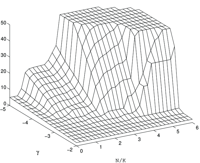
Figure 8: Surface of maximum algorithm size $KQ$ as a function of $\gamma$ and scale-up $N/K$, at $\epsilon=\gamma/100$ and $t_{m}=25$. All the axes have logarithmic scales, labeled in powers of 10. The surface has been truncated at $KQ=10^{50}$ to bring out the lower portions.

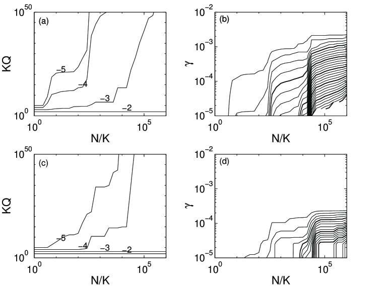
Figure 9: (a),(c): Lines of constant $\gamma$, for $\log_{10}\gamma=-2,-3,-4,-5$; (b),(d): contours of constant $KQ$. (a), (b) for the case plotted in figure 8, which has $\epsilon=\gamma/100,\;t_{m}=25$. (c), (d) for the case $\epsilon=\gamma,\;t_{m}=25$. The contours are at $10^{10}$, $10^{20}$, $10^{30}$, etc.; every 5th contour is shown with a thicker line.

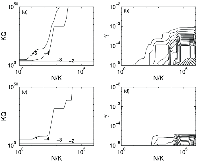
Figure 10: As figure 9, but for the case $\epsilon=\gamma$ and (a), (b): $t_{m}=1$; (c), (d): $t_{m}=100$.

The threshold result is indicated by the cliff at $\gamma\simeq 2\times 10^{-3}$ on the surface shown in figure 8, but this cliff is not the only important feature of the surface. Equally significant are the cliffs at $N/K\simeq 10$ and $N/K\simeq 1000$. The first indicates that large algorithms ($KQ\sim 10^{10}$) are possible for a modest scale-up once the gate noise rate is $\leq 10^{-4}$ (at $\epsilon=\gamma/100$), by using a BCH code, and the second cliff indicates that at the same noise rate a scale-up of a few thousand allows very large algorithms ($KQ\sim 10^{40}$), using the Golay code concatenated once with a BCH code.

The really huge values of $KQ>10^{20}$ should be interpreted as an indication not that such large algorithms can necessarily succeed, but rather that their failure will be for some other reason not considered here, such as technical or environmental problems causing correlated failure over many (e.g. hundreds of) qubits.

Comparing figure 9b with figure 9d, it is seen that increasing $\epsilon/\gamma$ from 0.01 to 1 at fixed $t_{m}$ has the effect approximately of shifting the surface in the direction of smaller $\gamma$ by an order of magnitude. Comparing figure 9d with figure 10d, it is seen that an increase in $t_{m}$ from 25 to 100 at $\epsilon=\gamma$ has the effect approximately of shifting the surface in the direction of smaller $\gamma$ by almost another order of magnitude.

It should be re-emphasized that all the noise rates quoted apply to non-local gates. They represent not the noise of a gate between neighbouring qubits, or during the time for such a gate, but the noise associated with a gate on qubits separated by some distance which depends on the code and on the structure of the computer. This distance has been discussed in 02:SteaneB , where it is found that for certain reasonable choices of the layout of the computer, the tolerated noise for a computer allowing only nearest-neighbour coupling is expected to be about an order of magnitude smaller than the tolerated noise for non-local gates which has been given here. Also, in the case of only nearest-neighbour couplings, at any given time-step in the $G,V$ networks, most ancilla qubits which are said to be ‘resting’ in the present discussion will be involved in one or more swap operations. A rough indication of the impact of this is obtained by letting the memory noise parameter $\epsilon$ in the present discussion include a contribution from the imprecision of swap gates.

A further assumption underlying all the results quoted is that the computing device allows as much parallelism in its operation as is logically possible for the networks considered. A reduction in the available parallelism can be compensated to some extent by a reduction in the memory noise.

VII Conclusion

The main results of this paper are figures 7 to 10, the set of equations (8)–(26), the network details set out in table 1, and related insights such as the good performance of the 23-bit Golay code, and the role of the measurement time $t_{m}$.

The fundamental reason why the crash probabilities fall to such low values is that uncorrelated and stochastic noise has the special property that the likelihood of a cluster of failures falls exponentially with the size of the cluster. There are two main reasons why in practice the noise will not be like this: qubit-qubit interactions and the technical details of the machinery used to supply the gate operations. The former are probably not too big a problem, since the strength of many-body Hamiltonians typically falls very rapidly with the number of bodies (see comments in section I.1). The latter can be tackled by standard coding techniques such as random coding, interleaving and concatenation. This implies that a study such as the present one should be regarded merely as a starting point for the complete structure of the computer. One method to suppress correlations is to use a low-level encoding such as $\left|{0}\right>_{L}=\left|{0101}\right>-\left|{0110}\right>+\left|{1001}\right>-\left|{1010}\right>$, $\left|{1}\right>_{L}=\left|{0101}\right>+\left|{0110}\right>-\left|{1001}\right>-\left|{1010}\right>$; this is a decoherence-free subspace for $ZZII$, $IIZZ$ and $XXXX$ operators and so is unaffected by joint $Z$-rotation of adjacent pairs of bits and joint $X$-rotation of quadruplets of bits.

Further work in this area could address the following issues. Does the error propagation directly between data blocks contribute significantly to the crash probability, when recoveries are placed in an optimal way as described in section 3? How well does the simple noise model capture the main features of noise and imprecision in particular physical examples? To what degree are error processes present whose effects add coherently rather than incoherently as assumed here? How much correlation and non-stochastic behaviour is found in practice? Further numerical simulations could be carried out on larger codes, mainly to test equations (10), (11). The cost of moving information around, and the transport distances required in QEC networks, could be further analyzed so that noise the tolerance for nearest-neighbour interactions can be calculated. The performance of further encoding to suppress correlated noise could be studied.

Appendix A: code construction

code	type	$n$	$k$	$d$	$w$	$N_{A}$	r
number
0	None	1	1	1	–	–	–
1	Hamming	7	1	3	3	12	3
2	Golay	23	1	7	11	77	4
3	,,	21	3	5	7	63	4
4	BCH	31	11	5	15	122	4
5	QR	47	1	11	15	281	5
6	,,	45	3	9	15	255	4
7	,,	43	5	7	15	229	4
8	BCH	63	27	7	27	350	4
9	,,	63	39	5	27	328	4
10	QR	79	1	15	27	801	5
11	,,	77	3	13	27	759	5
12	,,	75	5	11	27	713	5
13	QR	103	1	19	31	1265	6
14	,,	101	3	17	31	1215	5
15	,,	99	5	15	31	1165	5
16	,,	97	7	13	31	1119	5
17	BCH	127	29	15	47	1939	5
18	,,	127	43	13	47	1802	5

Table 1: Parameters of codes considered in the text. The code constructions are outlines in appendix A. The parameters $w$ and $N_{A}$ are the maximum weight of a row or column of the latin rectangle for $A$, and the number of $1$’s in $A$, respectively. The number of gates which act in parallel in most time-steps of the generation or verification network of a given ancilla is $N_{A}/w$. The final column gives the value of $r$ which was found to be optimal when $\gamma=100\epsilon=10^{-4}$, $t_{m}=25$, with $r-1=r^{\prime}=r^{\prime\prime}+1$.

Table 1 lists the parameters of the codes considered in the text. The values of $[[n,k,d]]$ are readily available from standard texts such as Bk:Macwilliams , but the values of $w$ and $N_{A}$ have to be obtained by examining the check matrices of the classical codes. These were created using standard methods, see Bk:Macwilliams chapters 7, 9, 16. The parity check matrix of a $[n=2^{m}-1,k_{c},d]$ classical BCH code was created by letting $f$ be equal to an $m$’th-order polynomial which is a factor of $1+x^{n}$ over GF$(2)$. The check matrix consists of a matrix of powers of $f$, where each entry is replaced by a column of $m$ bits giving the coefficients in the polynomial $f^{j}$.

For a quadratic residue code having $n$ a prime which is one less than a multiple of 4, the coefficients $f_{i}$, $0\leq i\leq n-1$, are defined to be 0(1) if $i$ is a quadratic residue (non-residue) respectively, modulo $n$, and $f_{0}=1$. The generator matrix is equal to the $n\times n$ circulant matrix $G_{ij}=f_{j-i}$.

Further codes listed were obtained by deleting two columns from the generator matrix of the classical code, to go from $[[n,k,d]]$ to $[[n-2,k+2,d-2]]$, see 96:SteaneC ; 98:Calderbank .

Once the check matrix or generator matrix was obtained, it was converted into the $(IA)$ form, and then $w$ and $N_{A}$ could be obtained.

Appendix B: ancilla preparation statistics

The ancilla preparation and verification was studied using the Monte-Carlo method described in section III. The method was to use the noisy $G$, $V$ and ancilla–data coupling networks to extract a single syndrome from a data block which was prepared with no errors. This was repeated many times (starting from an error-free data block each time) and the various syndromes obtained were counted, for values of $\gamma$ in the range $10^{-5}<\gamma<10^{-2}$.

Under the conditions of the numerical experiment, the obtained syndrome should be zero. The non-zero syndromes indicate the errors produced by the preparation/verification network which were not detected during verification, and the further errors produced by the coupling of ancilla to data, the final Hadamard gates on the ancilla, and the measurements.

Let the syndromes be $\{s\}$. The program gives the probabilities $P_{s}(\gamma,\epsilon,t_{m})$ of obtaining each $s$, for a range of values of $\gamma$ at given $\epsilon/\gamma$ and $t_{m}$. I fit each set of results to a power-law

$$P_{s}(\gamma)=a_{s}\gamma^{c_{s}}$$ (27)

where the fitted parameters $a_{s}$ and $c_{s}$ depend on $\epsilon/\gamma$, $t_{m}$ and the code under consideration. Only values of $P_{s}$ less than $0.01$ were included in the fit, in order to avoid the non-power-law dependence when $P_{s}$ approaches 1. I can thus examine the statistics of the ancilla preparation in some detail by examining the set of coefficients $a_{s}$, $c_{s}$.

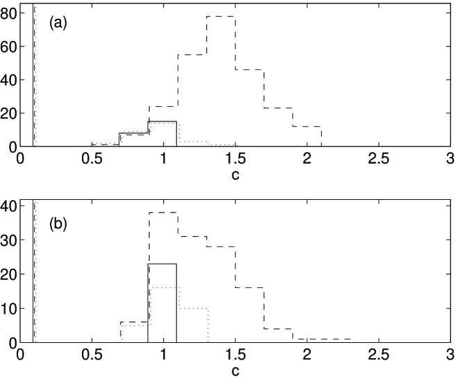
Figure 11: Distribution of $c_{s}$ values giving the power law dependence of the probability of obtaining errors in the prepared ancilla, as a function of gate noise rate. The example given is for the Golay code at $t_{m}=1$ and (a) $\epsilon=\gamma$, (b) $\epsilon=\gamma/100$. Three histograms are plotted, showing the distribution for errors of weight 1 (full line), 2 (dashed line) and 3 (dotted line).

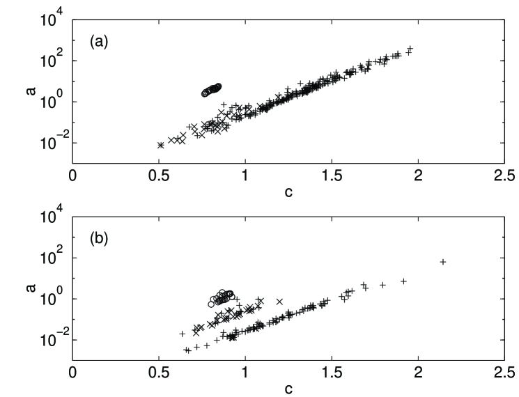
Figure 12: The fitted coefficients of equation (27) for all the ancilla errors observed in a large number of runs of the Monte-Carlo simulation for the Golay code, at $t_{m}=1$. (a) $\epsilon=\gamma$, (b) $\epsilon=\gamma/100$. The symbols indicate the error weight 1 (o), 2 ($+$) or 3 ($\times$).

Figure 11 shows histograms giving the distribution of $c_{s}$ values in the case of the Golay code, for $t_{m}=1$. The obtained syndromes are first divided into sets, defined by the weight of the coset leaders. I give the histogram for each set. This shows the power-law dependence for preparing an ancilla with an error of each weight. For weight 1, I obtain $c_{s}=1$, as expected: the most likely cause of a single error is a single failure. For weight 2, $c_{s}$ falls between 1 and 2, indicating that the most likely weight-2 errors are caused by single failures or double failures in roughly equal proportions. For weight 3, most $c_{s}$ values are close to 1, indicating that those weight-3 errors which can be produced by a single failure are the most likely ones to occur.

Figure 12 shows plots of $a_{s}$ verses $c_{s}$. There are two features which stand out. First, there is a correlation between $a_{s}$ and $c_{s}$, for the syndromes of each error weight, such that $a_{s}$ increases by a factor of order $10^{3}$ when $c_{s}$ increases by 1. This means that the $P_{s}$ having small $c_{s}$ will be more likely than those having large $c_{s}$ when $\gamma<10^{-3}$, which is the regime of interest. Therefore errors (of whatever weight) caused by single failures are the main ones I need to account for in attempting to model the behaviour.

The second feature is that each weight-1 error is much more likely to be produced than any individual weight-2 error. This is to be expected: there are several single failure locations which can produce a given weight-1 error in the ancilla, but only a smaller number which can produce any given error of weight $>1$.

Note that at $\epsilon=\gamma/100$, fig. 12 shows that most individual errors of weight 3 are more likely than individual errors of weight 2, but fig. 11 shows that there are fewer of them. This suggests the weight-3 errors here are caused by gate failure in the preparation and verification networks, while most of the weight-2 errors are caused by memory failure.

$\epsilon/\gamma$	$t_{m}$	$a$	$a^{\prime}$	$a+a^{\prime}$	$P_{Z\rm a}$
1	1	196	36	214	$243\gamma$
0.01	1	65	21	86	$103\gamma$
1	25	509	54	563	$609\gamma$
0.01	25	65	16	81	$106\gamma$

Table 2: Linear fit coefficients $a$, $a^{\prime}$ for the probabilities of ancilla error of weight 1 ($a$, column 3) and weight $>1$ ($a^{\prime}$, column 4), obtained from the numerical calculations at two values of $\epsilon/\gamma$ and of $t_{m}$. The final column gives the probability of any ancilla error as estimated by equation (8).

A further statistic extracted from the calculations was the total probability $P_{w}$ of obtaining any ancilla error of given weight $w$, for weights between 1 and 4. This probability was fitted to a power law (as a function of $\gamma$ at fixed $\epsilon/\gamma$). The powers obtained were close to 1 (e.g. at $t_{m}=1$ the powers were $0.97,1.6,1.4,1.1$ for weights $1,2,3,4$ respectively, when $\epsilon=\gamma$, and $0.93,1.2,1.1,1.1$ when $\epsilon=\gamma/100$.) In view of this and of the fact noted above, that errors caused by single failures dominate the statistics when $\gamma<10^{-3}$, modeling these probabilities by a linear dependence on $\gamma$ will capture the main features. Table 2 gives the fitted coefficient $a$ in the single-parameter linear fit $P_{w=1}=a\gamma$, and $a^{\prime}$ in the fit $P_{w=2}+P_{w=3}+P_{w=4}=a^{\prime}\gamma$, for two different values of $\epsilon/\gamma$ and two different values of $t_{m}$. I expect the net probability $P_{Z{\rm a}}=\sum_{w}P_{w}$ for the ancilla to have some error to be as given by equation (8). The table shows that the numerical results are fitted reasonably well by this model.

The other feature of the analysis presented in section IV which I need to confirm is the value of $P_{\rm ws}$. This is the probability of a crash caused by several successive ancillas conspiring to agree on a wrong syndrome. Suppose the ancillas all suffer from the same error vector $e$. When they couple to the data, they pick up the error vector $d$ of the data bits, to give a net error vector $e+d$. Assuming $e+d$ is correctable, the correction applied to the data will be $e+d$, which leaves the error $e$ in the data. If $e$ has small weight, this will not cause a crash, and furthermore if $e$ has weight 1, it will only add a further small contribution (scaling as the failure rates raised to the power $r^{\prime}$) to the coefficient for single data errors, which is essentially harmless 02:SteaneA . It follows that $P_{\rm ws}$ can be estimated as the probability that $r^{\prime}$ ancillas all have the same error $e$ whose weight is greater than 1. Such errors are caused mostly by that part of the $G$ and $V$ networks which takes place before $V$ is completed, in which $X$ and $Y$ errors are mostly detected. The probability for any given $e$ is therefore either $\gamma/3$ or $\epsilon/3$, depending on whether it was caused by a gate failure or a memory failure. The number of different $e$ of weight $>1$ that can be caused by a single failure is overestimated by $N_{GV}$, ($N_{h}$), for those $e$ caused by gate failure (memory failure) respectively, hence I obtain the approximate value for $P_{\rm ws}$ given in equation (18). (For the Golay code the numerical study indicated for that case the true numbers were $\simeq N_{GV}/4$ ($\simeq N_{h}/4$).) If $t_{m}$ is sufficiently large, then the memory noise while verification bits are measured will be such that a double failure in this part of the network is as likely as a single failure elsewhere; such a contribution can be neglected as long as $(t_{m}\epsilon)^{2}\ll\gamma_{2}$. If the measurement failure probability $\gamma_{m}$ is sufficiently large then double measurement failures will be significant; their contribution is small as long as $\gamma_{m}^{2}\ll\gamma_{2}$.

- (1) P. W. Shor, Phys. Rev. A 52, R2493 (1995).
- (2) A. M. Steane, Phys. Rev. Lett. 77, 793 (1996).
- (3) A. R. Calderbank and P. W. Shor, Phys. Rev. A 54, 1098 (1996).
- (4) A. M. Steane, Proc. Roy. Soc. Lond. A 452, 2551 (1996).
- (5) P. W. Shor, in Proc. 35th Annual Symposium on Fundamentals of Computer Science (IEEE Press, Los Alamitos, 1996), pp. 56–65, quant-ph/9605011.
- (6) D. P. DiVincenzo and P. W. Shor, Phys. Rev. Lett. 77, 3260 (1996).
- (7) J. Preskill, Proc. R. Soc. Lond. A 454, 385 (1998).
- (8) D. Gottesman, Physical Review A 57, 127 (1998), quant-ph/9702029.
- (9) D. Gottesman and I. L. Chuang, Nature 402, 390 (1999), quant-ph/9908010.
- (10) A. Y. Kitaev, in Quantum Communication, Computing and Measurement (Proc. 3rd Int. Conf. of Quantum Communication and Measurement) (Plenum Press, New York, 1997), pp. 181–188.
- (11) E. Knill, R. Laflamme, and W. H. Zurek, Science 279, 342 (1998).
- (12) A. M. Steane, Nature 399, 124 (1999), quant-ph/9809054.
- (13) A. M. Steane, Fortschritte der Physik (Prog. Phys.) 46, 443 (1997), quant-ph/9708021.
- (14) A. M. Steane, submitted for publication (2002), quant-ph/0202036.
- (15) D. Aharonov and M. Ben-Or, in Proc. 29th Ann. ACM Symp. on Theory of Computing (ACM, New York, 1998), p. 176, quant-ph/9906129, quant-ph/9611025.
- (16) A. M. Steane, Phys. Rev. Lett. 78, 2252 (1997), quant-ph/9608026.
- (17) A. Y. Kitaev, (1997), quant-ph/9707021.
- (18) D. Gottesman, Ph.D. thesis, California Institute of Technology, 1997.
- (19) A. M. Steane, Quant. Inf. and Comp. 2, 297 (2002), quant-ph/0203047.
- (20) A. M. Steane, in Decoherence and its Implications in Quantum Computation and Information Transfer (IOS Press, Amsterdam, 2001), pp. 284–298, quant-ph/0304016.
- (21) E. Knill and R. Laflamme, Phys. Rev. A 55, 900 (1997), quant-ph/9604034.
- (22) E. Knill, R. Laflamme, and L. Viola, Phys. Rev. Lett. 84, 2525 (2000), quant-ph/9908066.
- (23) R. Alicki, M. Horodecki, P. Horodecki, and R. Horodecki, PhysRevA 65, 062101 (2002), quant-ph/0105115.
- (24) C. Zalka, (1999), quant-ph/9612028 v2.
- (25) W. H. Press, S. A. Teukolsky, W. T. Vetterling, and B. P. Flannery, Numerical Recipes in C, the art of scientific computing (Cambridge University Press, England, 1994).
- (26) J. Preskill, in Introduction to Quantum Computation, edited by H.-K. Lo, S. Popescu, and T. Spiller (World Scientific, Singapore, 1998), pp. 213–269, quant-ph/9712048.
- (27) F. J. MacWilliams and N. J. A. Sloane, The Theory of Error-Correcting Codes (North-Holland, Amsterdam, 1977).
- (28) A. M. Steane, Phys. Rev. A 54, 4741 (1996).
- (29) A. R. Calderbank, E. M. Rains, P. W. Shor, and N. J. A. Sloane, IEEE Transactions on Information Theory 44, 1369 (1998).